1. Introduction
Over the past decade, research in sound classification and recognition has gained in popularity and rapidly broaden in its application from the more traditional focus on speech recognition [
1] and music genre classification [
2] to biometric identification [
3], computer-aided heart sound detection [
4], environmental audio scene and sound recognition [
5,
6], biodiversity assessment [
7], human voice classification and emotion recognition [
8], English accent classification, and gender identification [
9], to list a few of a wide range of application areas. As with research in pattern recognition generally, the features fed into classifiers were initially engineered, which, in the case of sound applications, meant extracting from raw audio traces such descriptors as the Statistical Spectrum Descriptor and Rhythm Histogram [
10].
In the past decade, researchers began exploring the possibility of visually representing audio signals to apply more powerful image classification descriptors and techniques. Initially, visual representations of audio traces centered around the display overtime of the frequency spectrum: examples of these representations include the spectrogram [
11] and Mel-frequency Cepstral Coefficients spectrogram [
12]. Although a spectrogram is typically a graph with two dimensions (time and frequency), additional dimensions can be included, such as pixel intensity [
13], which includes at each time step the representation of an audio signal’s amplitude in a specific frequency. Initially, popular texture descriptors, such as Haralick’s Grey Level Co-occurrence Matrices (GLCMs) [
14], Gabor filters [
15], and Local Binary Patterns (LBP) [
16] and its variants [
17] were extracted from these spectrograms for the task of music genre classification [
18,
19,
20]. Fusions of a large set of state-of-the-art texture descriptors were then experimentally applied to spectrograms, and certain combinations were shown to enhance further the accuracy of music genre classification [
2].
The rise in popularity of deep learning due to affordable graphic processing units (GPUs) changed the trajectory in machine learning research [
21]. Deep learners, such as the convolutional neural network (CNN), produced far superior results to most other classifiers when it came to image classification [
22]. Consequently, more attention was placed on representing acoustic traces through visual representations so that deep learning approaches could be applied. Engineered features diminished in importance since deep classifiers learn which patterns perform best for a specific problem during the training process. However, engineered features have been shown to augment deep learning approaches when fused. Early work with CNNs applied to visual representations obtained state-of-the-art in chord detection and recognition [
23,
24] and in music genre classification [
25]. In [
25], for example, spectrograms were converted into GCLM maps and trained on CNNs. In [
26], canonical approaches, such as LBP-trained SVMs were fused with CNNs and shown to outperform previous systems.
Another development in sound classification involves the design of deep learners and feature sets specific to audio classification. For example, in [
27], the authors explored variations in CNN architecture and parameters; in [
28] a novel
sparse coding CNN was developed and shown to perform well if not better than the state-of-the-art for sound event recognition and retrieval. Also of note is the hybrid multimodal deep learning approach proposed in [
29] for multilabel music genre classification that combined album cover images, reviews, and audio tracks; this system was shown to outperform the single-modality approaches. In [
30] the authors present a gated CNN and a temporary attention-based classification system for audio classification from weakly labeled data.
When it comes to animal sound classification, the focus of this study, fusions of CNNs with other methods to classify animals have been evaluated in [
31] and [
32] for fish identification using the Fish and MBARI benthic animal dataset and in [
33] for bioacoustic bird species classification using a dataset of audio samples from 43 species. In [
31], the authors combined engineered features with CNNs, and in [
33], deep learning was combined with shallow learning. Both demonstrated that the fusions performed better than the standalone approaches.
Animal sound classification is a vibrant area of research. Many benchmark datasets are available for a variety of animals, such as bats [
34], birds [
34,
35], whales [
36], cats [
37], and frogs [
35]. In the literature, animal audio classification is broadly divided into two categories: the CNN approach discussed above and fingerprinting [
38], which involves a compact audio representation for comparing audio segments in terms of similarity and dissimilarity [
39]. Both approaches, however, suffer from limitations: fingerprinting can only find exact matches, and CNNs require large datasets for accurate training; many animal datasets are small because of the difficulty of collecting samples.
The superiority of combining the deep learning approach with fingerprinting is demonstrated in [
40], where a Siamese Neural Network (SNN) produced semantic descriptions of audio signals. SNNs have been applied to sound classification in [
40,
41,
42] and have the advantage over the canonical CNN in their ability to generalize. In [
43], a system was developed based on dissimilarity spaces, such as that proposed in [
44] for brain image classification, where a distance model was learned by training a SNN [
45] on dissimilarity values. This system combined several clustering approaches to obtain a dissimilarity space; each pattern was represented in such a space, and the resulting descriptors were used to train a general purpose classifier (SVM). The clustering methods transformed the spectrograms in a bird [
46] and cat [
37,
47] dataset to a set of centroids that were used to generate a vector space representation for each pattern. This vector was then used to train an SVM. Results showed that this approach worked better than the standalone CNNs.
The system proposed in this work is similar to [
43] in that it generates a dissimilarity space from the training set using an SNN to define a distance function from the input spectrograms. The objective at this point in the process is to maximize the distance separating the patterns of the different classes. Unlike [
43], however, four different CNN architectures are selected for the twin classifiers, and both the original input spectrograms and the spectrograms processed by Heterogeneous Auto-Similarities of Characteristics [
48] make up the inputs to the SNNs. In the testing phase, the unknown pattern is compared to the centroids of the dissimilarity space using the different SNNs for comparing two samples and measure their dissimilarity. Although it is the case that the entire training set can function as the centroids of the dissimilarity space, it is desirable to reduce dimensionality by selecting a smaller number of prototypes. In this work, both a supervised and unsupervised clustering algorithm are used to reduce dimensionality. The dissimilarity space represents each input (both the original and the processed spectrograms) by its distance from each of the centroids, or prototypes, a distance that is learned by the SNNs. In other words, the SNNs compare a given spectrogram to each of the centroids to obtain a dissimilarity feature vector. A support vector machine (SVM) is then trained on these features.
The approach taken in this paper is evaluated on the same animal vocalization datasets as in [
43], i.e., on cats [
37] and birds [
7]. In addition, the system is tested on the challenging benchmark dataset for Environmental Sound Classification (ESC-50) [
49]. As in [
43], the most effective system is the result of a fusion of classifiers, i.e., the sum rule of SVMs trained on different dissimilarity spaces generated by changing the value of
k in the clustering approaches and network topologies. Performance is compared with both the state-of-the-art as well as with fusions with the state-of-the-art. Results demonstrate the power of using dissimilarity spaces based on an ensemble of SNNs, particularly when coupled with a standard CNN approach. The MATLAB code of the proposed method is freely available at
https://github.com/LorisNanni.
The remainder of this paper is broken down into the following sections. In
Section 2, a detailed overview of the proposed approach is provided; in
Section 3, SNN is discussed along with the different CNN architectures that make up the subnetworks. In
Section 4, the supervised and unsupervised clustering methods are outlined. In
Section 5, experimental results are presented along with comparisons with the state-of-the-art. The paper concludes in
Section 6 with an overview and some suggestions for future research.
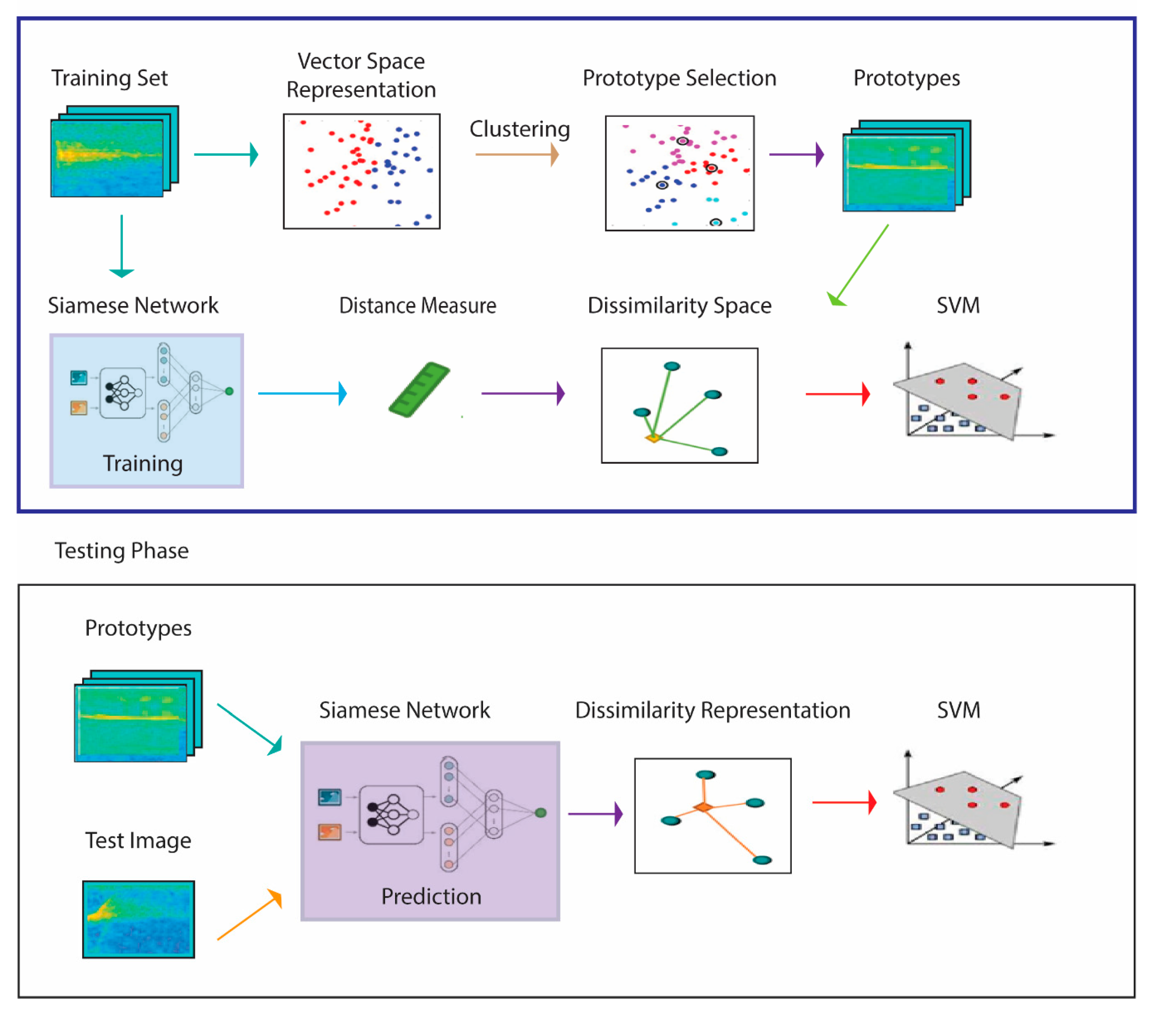
2. Proposed System
The system presented here for spectrogram classification extends that proposed in [
43] and is schematized in
Figure 1, which illustrates the approach using one SNN. The pseudocode in Algorithms 1 and 2 that correspond to
Figure 1 are detailed in the remainder of this section.
The process begins by generating a similarity space during the training phase via a learning distance measure from a set of prototypes . The distance measure is learned by four SNNs trained (1) to maximize the similarity between pairs of spectrograms belonging to the same class and (2) to minimalize the similarity for pairs of spectrograms belonging to different classes. The set of prototypes generated in this phase are the centroids of the clusters produced by a clustering approach. What results is a feature vector that represents training sample in the dissimilarity space, where a given is the distance between and the prototype . Once these features have been calculated, they are used to train an SVM classifier.
In the testing phase, each unknown pattern is represented by its projection in a dissimilarity space: the descriptor is obtained by calculating the pattern distance to the set of prototypes
and the resulting feature vectors of the input images are then classified by SVM. In our experiments, we test both spectrograms and HASC [
48], a 2D descriptor extracted from the spectrogram, as the input of the classification process. The method for extracting HASC is outlined in
Section 2.5.
| Algorithm 1. Training phase |
Input: Training images (imgsTrain), training labels (labelTrain), number of training iterations
(trainIterations), batch size (trainBatchSize), number of centroids (k), and clustering technique (type). |
| Output: Trained SNN (tSNN), set of centroids (C), and trained SVM (svm). |
| 1: tSNN ← trainSiamese(imgsTrain, labelTrain, trainIterations, trainBatchSize) |
| 2: p ← Clustering(imgsTrain, labelTrain, k, type) |
| 3: F ← getDissSpaceProjection(imgsTrain, P, tSNN) |
| 4: tSVM ← trainSvm(labelTrain, F) |
| Algorithm 2. Testing phase |
| Input: Test images (imgsTest), trained SNN (tSNN), Set of centroids (C), Trained SVM (tSVM). |
| Output: Actual test labels (labelTest). |
| 1: F ← getDissSpaceProjection (imgsTest, P, tSNN) |
| 2: labelTest ← predictSvm (F, tSVM) |
2.1. Siamese Neural Network Training
To define a similarity measure inside the Dissimilarity Space, a Siamese Network is trained to compare a couple of spectrograms and return a similarity value that is the greater value if they belong to the same class and the lower value if they belong to different classes. The pseudocode for training an SNN, which is called in step 1 of Algorithm 1, is reported in Algorithm 3. The SNN architecture is defined in steps 2 and 3 (more details are given in
Section 3). The training process consists in repeating Steps 5–8: random extraction of
batchSize spectrogram pairs from the training set (via the function GETBATCH), computation of loss and gradients for each pair passed to the SNN, and upgrade of the SNN accordingly (i.e., the subnet and the fully connected (FN) layer of the Siamese network).
| Algorithm 3. Siamese training pseudocode |
| Input: Training image (trainImgs), training labels (trainLabels), batch size (batchSize), and iterations (numberO f Iterations). |
| Output: Trained SNN (tSNN). |
| 1: function TRAINSVM |
| 2: subnet←NETWORK([inputLayer,..., FullyConnectedLayer]) |
| 3: f cWeights←randomWeights |
| 4: for iteration from 1 to numberO f Iterations do |
| 5: X1, X2, pairLabels← getBatch (trainImgs, trainLabels, batchSize) |
| 6: gradients, loss← Evaluate(subnet, X1, X2, pairLabels) |
| 7: Update(subnet, gradients) |
| 8: Update(f cWeights, gradients) |
| 9: end for |
| 10: return tSNN←subnet, f cWeights |
| 11: end function |
| Note: if SNN fails to converge on the training set, the training phase is repeated. |
2.2. Prototype Selection
Prototype selection involves extracting a total of
k prototypes from the training set in order to reduce the dimensionality of the dissimilarity space, which would be too high to maintain each training sample as a prototype. Dimensionality can be reduced by employing clustering techniques to calculate
k centroids. In this work, we perform both prototype selection separately for each class (
kc prototypes per class) and via global (i.e., unsupervised) clustering (
k prototypes): in both cases, results are compared considering the same final dimension. Algorithm 4 presents the pseudocode for prototype selection. As can be observed, a clustering technique is selected from a set of four possible clustering methods, each of which is employed separately to cluster the training samples. For the sake of space, only the pseudocode for the supervised clustering methods is included, though it should be noted that this work used both supervised and unsupervised clustering approaches.
| Algorithm 4. Clustering pseudocode |
| Input: Training images (imgsTrain), training labels (labelTrain), number of clusters (k), and clustering technique (type). |
| Output: Centroids P. |
| 1: function Clustering |
| 2: numClasses←number of classes from labelTrain |
| 3: kc←k/numClasses |
| 4: for i from 1 to numClasses do |
| 5: images←images of the class i from imgsTrain |
| 6: switch type do |
| 7: case “k-means” Pi ← KMeans(imgs,kc) |
| 8: case “k-medoids” Pi ← KMedoids (imgs,kc) |
| 9: case “hierarchical” Pi ← Hierarchical (imgs,kc) |
| 10: case “spectral” Pi ← Spectral (imgs,kc) |
| 11: P←P ∪Pi |
| 12: end for |
| 13: return P |
| 14: end function |
2.3. Projection in the Dissimilarity Space
Classically, classifiers are trained to predict patterns within a feature space. It is also possible, as demonstrated here, for patterns to be projected in a dissimilarity space such that each pattern
is characterized by its dissimilarity to a set of prototypes
and by a dissimilarity vector defined as
where the similarity of pattern
is obtained using a trained SNN.
The projection of a set of images (from the training or the testing set) into a dissimilarity space
is described in Algorithm 5. Each image of the input set (stored in the variable
X, see step 3) is compared with the
k prototypes (stored in
P) according to the dissimilarity measure learned by the trained SNN (PREDICTSIAMESE function, see step 4). The number of centroids is a parameter, and different values of
were tested (depending on the number of classes
):
. The output is the feature space
F that includes the projections of all the input images
imgs.
| Algorithm 5. Projection in the Dissimilarity space pseudocode |
| Input: Images (imgs), Centroids (P), number of centroids (k), and trained SNN (tSNN). |
| Output: Feature vectors (F). |
| 1: function getDissSpaceProjection |
| 2: for j from 1 to SIZE(imgs) do |
| 3: X←imgs[j] |
| 4: F[j]← predictSiamese (tSNN, X, P) |
| 5: end for |
| 6: return F |
| 7: end function |
2.4. Classification by SVM
SVM [
50] is a well-known binary learner that represents training samples as points in space. The goal of SVM training (function TRAINSVM) is to find at least one hyperplane such that it separates the data that belongs to each of the two classes. Prediction (function PREDICTSVM) is accomplished by mapping an unseen pattern to the side of the hyperplane representing the class for a given data point.
SVM, as defined above, does a poor job discriminating input that is not linearly separable in its original space. This difficulty can be overcome by selecting kernel functions that map the data into a higher-dimensional space where separation is possible. In this work, we chose a radial basis function kernel to map a single vector to a vector of higher dimensionality.
Although SVM is binary, it can be applied to nonbinary or multilabel problems by training an ensemble of SVMs and combining their decisions. In the experiments reported here, the One-Against-All method is used, where an SVM is trained systematically to distinguish each class against all the others combined. The pattern is then predicted to belong to that class that produces the highest confidence score.
2.5. Heterogeneous Auto-Similarities of Characteristics (HASC)
HASC [
48] is applied to heterogeneous dense feature maps. It encodes linear relations by covariances (COV) and nonlinear associations with entropy combined with mutual information (EMI). Three reasons for considering covariance matrices as descriptors are as follows: (1) they are low in dimensionality, (2) robust to noise (but with the exception that outlier pixels can render them more sensitive to noise), and (3) the covariance among two features is optimally able to encapsulate the features of the joint PDF (but with the caveat that they be linked by a linear relation). HASC obviates these limitations by combining COV with EMI.
The entropy (E) of a random variable measures the uncertainty of its value, and the mutual information (MI) of two random variables captures their generic linear and nonlinear dependencies. The way HASC utilizes these advantages is by dividing an image into patches from which it generates an EMI matrix (
, such that the main diagonal entries encapsulate the amount of unpredictability of the
features. The off-diagonal entries (element
capture the mutual dependency between two features, that is, the
-th and
-th feature. HASC is the concatenation of vectorized EMI and COV. Specifically, the MI of a pair of random variables
is
where
, and
are the PDF of
, the PDF of
, and their joint PDF, respectively. If
, then MI is the entropy of
:
If there exists a finite set
of realization pairs, MI can be estimated as a sample mean inside the logarithm, thus:
A fast and efficient method for calculating from the
realizations the probabilities inside the logarithm is to estimate them by building a joint 2D normalized histogram of values
and
, such that each
is estimated taking the value of the 2D histogram bin containing the pair
. In this way,
and
can be estimated by summing all the bins corresponding to
and
, respectively. Thus, the
-th component of the EMI matrix related to the patch
can be defined as
where
(…) and
(.) are the probabilities estimated with the histogram and
is the
-th feature at pixel
.
In this study, HASC is extracted from the whole spectrogram. Given the function HASC, the output FEAT is a three-dimensional matrix () containing the features extracted from the image ( is the number of low-level features). The number of bins used to evaluate the histograms in the EMI computation is 28, and the number of low-level features is 6 (default parameters). FEAT is reshaped to build the vector [FEAT (:,:,1) FEAT (:,:,2); FEAT (:,:,3) FEAT (:,:,4); FEAT (:,:,5) FEAT (:,:,6)], and is resized to the right dimension for the input into a CNN.
4. Clustering
Clustering is a procedure that divides unlabeled patterns into groups that maximize the commonality between members within a group and their differences with members belonging to other groups. Clustering techniques often calculate the mean vector, or centroid, of all the patterns within a cluster when forming the clusters. Centroids encapsulate salient characteristics of patterns belonging to a cluster; for this reason, they can be used to reduce the dissimilarity space size without losing too much important information. Even more information can be retained if the number of centroids representing each class is increased.
Both supervised and unsupervised clustering approaches are considered here. If clusters are extracted with a supervised approach, then, in each of classes, clusters are extracted using unsupervised clustering on the training set. A description of the four clustering methods used in this study follows.
4.1. K-Means
K-means is one of the most popular clustering algorithms. It partitions patterns into k clusters by placing each observation into a cluster based on the nearest centroid (according to the Euclidean Distance measure).
The standard k-means algorithm involves four steps:
Randomly select a set of centroids from among the data points.
For each data point x remaining in the training set, compute the distance d(x) between it and the nearest centroid.
Recalculate new centroids via a weighted probability distribution.
Repeat Steps 2 and 3 until convergence.
4.2. K-Medoids
K-medoids is a clustering technique that follows the same general logic behind k-means but differs in the specific way it partitions data points into clusters: K-medoids minimizes the sum of distances between a given pattern and the center of that pattern’s cluster. In short, the center of a cluster in K-Means ends up being the centroid of the cluster, but the center in K-Medoids is a member (medoid) of the cluster. In other words, a medoid is that member in a cluster whose sum of distances from all other members is minimal.
The standard K-medoids algorithm involves three steps:
Step one is a build-step where each k cluster is associated with a potential medoid. There are many ways to select the first medoid; the standard MATLAB’s implementation does this employing the k-means++ heuristic.
Step two is a swap-step where each point in a cluster is tested as a potential medoid by checking whether the sum of the within-cluster distances is smaller when using that point as the medoid. Every point is then assigned to the cluster with the closest medoid.
The last step repeats previous steps until convergence.
4.3. Spectral
Spectral clustering partitions data into clusters starting from the adjacency matrix representing the undirected similarity graph of the patterns. Each pattern is a node of the graph, and two nodes are connected only if their similarity is larger than a threshold (typically set to 0).
This clustering algorithm involves the following matrices:
The similarity matrix M, whose cell is the similarity value of two patterns (i.e., two spectrograms , );
The degree matrix
D, which is a diagonal matrix that is obtained by summing the rows of
M:
The Laplacian matrix L, which is defined as
The algorithm for spectral clustering is a five-step process:
Define a local neighborhood for each data point in the dataset (there are many ways to define a neighborhood; the nearest-neighbor method is the default setting in the MATLAB implementation of spectral clustering). Then compute the local similarity matrix of each pattern in the neighborhood.
Calculate the Laplacian matrix .
Create a matrix containing columns , …, , where the columns are the eigenvectors, i.e., the spectrums (hence the name), corresponding to the smallest eigenvalues of L.
Perform k-means or k-medoids clustering by treating each row of V as a datapoint.
Cluster the original pattern according to the assignments of their corresponding rows.
4.4. Hierarchical Clustering
Hierarchical clustering partitions data by creating a tree of clusters divided into n levels selected for the specific classification task. In general, hierarchical clustering is divided into two types:
Agglomerative, where each pattern corresponds to a cluster. A strategy to merge couples of clusters is defined as moving up the hierarchy: each cluster in the next level is the fusion of two clusters from the previous level.
Divisive, where a single cluster contains all patterns in the first level, then a splitting strategy is defined to halve clusters by moving down the hierarchy.
In this work, the agglomerative hierarchical approach is employed as this is the default MATLAB implementation. The MATLAB algorithm involves three steps:
Using a distance metric, find the similarity or dissimilarity between every pair of data points in the dataset;
Aggregate data points into a binary hierarchical cluster tree by fusing pairs of clusters according to their distance;
Establish the level of the tree where it is cut into k clusters.
The resulting prototypes are selected as the mean vectors of each cluster.
5. Experimental Results
The proposed approach is tested and compared with the canonical approaches with each using the testing protocol proposed by the authors of the datasets. The performance indicator is the classification accuracy and methods were tested on the following animal vocalization datasets:
BIRDz, which functioned as a control and a real-world audio dataset in [
46], a ten-run testing protocol is used; we have used the same split used by the authors of the dataset. The real-world tracks were collected from the Xeno-canto Archive (
http://www.xeno-canto.org/).
BIRDz includes a total of 2762 bird acoustic samples from 11 North American bird species plus 339 “unknown” samples that include noise and unknown species’ vocalizations. The observations are composed of five different spectrograms: 1) constant frequency, 2) frequency modulated whistles, 3) broadband pulses, (4) broadband with varying frequency components, and 5) strong harmonics. The dataset is balanced: the size of all the “bird” classes varies between 246 and 259; only the class “other” is a little larger.
CAT, [
37,
47] is a dataset that contains ten balanced classes of approximately 300 samples per class for a total of 2962 samples. The testing protocol is a 10-fold cross-validation. The ten classes represent the following cat vocalizations: (1) Resting, (2) Warning, (3) Angry, (4) Defense, (5) Fighting, (6)·Happy, (7) Hunting mind, (8) Mating, (9) Mother call, and (10) Paining. The average duration of each sample is approximately 4 s. Samples were garnered from such online resources as Kaggle, Youtube, and Flickr.
In this section, we report experiments aimed at evaluating the proposed system by varying several components: i.e., the input images (spectrograms or HASC images), the topology of the Siamese Network (NN1, NN2, NN3, NN4), the clustering algorithm (K-Means, K-Medoids, Hierarchical, Spectral), the clustering modality (unsupervised or supervised, i.e., clustering on the whole training set or on each class), and the number of prototypes (kc = 15, 30, 45, 60). For the training of the Siamese networks in our experiments, we have selected the training options suggested by the MATLAB framework for Siamese networks. This choice ensures that such values have not been overfitted on the selected dataset. The binary cross-entropy gives the loss function between the predicted score and the true label value. The parameters for ADAM optimization are the following: learning rate 0.0001, gradient decay factor 0.9, squared gradient decay factor 0.99. The number of iterations has been set at 3000 (without any early stop criterion).
In the first experiment, reported in
Table 2, only K-means clustering is explored. The results are obtained from the fusion by sum rule of the four SVMs trained using the dissimilarity spaces built with different values for
kc (15, 30, 45, 60). Performance is reported for only NN1 and NN2 (the first two network topologies) to reduce the computation time.
The ensembles in
Table 2 are obtained by varying the input data (Sp = spectrograms, HASC = HASC images), the type of clustering (unsupervised or supervised), and the network topology. The clustering method is fixed to K-means for all the methods, and the number of prototypes belongs to the following set (15,30,45,60). The column labeled
#classifiers recaps the number of classifiers in the ensemble, and the first column (“Name”) assigns a name to the ensemble.
The best average performance is obtained by the ensemble FA1_2 in the last row (which is the sum rule of the methods in the first eight rows). On the BIRD dataset, there is a boost in performance with NN1 and NN2 using the HASC images instead of the spectrograms, while on the CAT dataset, HASC images boost the performance of NN2 but not NN1.
The goal of the second experiment is to compare the clustering methods. To achieve this aim, in
Table 3, we report the performance of different clustering approaches using the HSup-2 approach (i.e., HASC images as input, NN2 as network topology, and unsupervised version of the clustering). The last row reports the ensemble F_Clu obtained as the sum rule among the above four approaches. F_Clu produces the highest performance, though this gain is only slightly higher than that of K-means. All the clustering algorithms are quite similar in performance. Since their fusion does not achieve a clear advantage against a single approach, in the next experiments, we use only the K-means strategy for clustering by varying the number of prototypes
kc.In
Table 4, the four network topologies are coupled with K-means clustering and HSup (i.e., HASC images as input and the unsupervised version of clustering). The last row, which reports the ensemble F_NN is obtained as the sum rule among the above four approaches, and it produces the average best performance on this test.
Even better results are obtained by combining by sum rule all the approaches reported in the previous tables: the combined performance on CAT is 85.76 and on BIRD 95.08. It is clear that the ensemble strongly outperforms a simple Sup-1. The superiority of one method over another is validated according to the Wilcoxon signed-rank test [
54]; F_NN outperforms each of the other methods with a
p-value of 0.05.
The following experiment is aimed at evaluating the possibility of creating ensembles by varying some parameters of the method. For a fair comparison among ensembles in
Table 5, the performance of an ensemble obtained by retraining Siamese HSup-1 (i.e., by using the same approach as that reported in
Table 2) is compared with ensembles obtained by varying the network topology. The results of
Table 5 indicate that changing the network topology introduces diversity in the ensemble: the comparison among ensembles of 4, 8, and 16 networks (see HSup-1
x), obtained from the topology NN1, and the ensembles named F_NN, obtained by varying the topology of the Siamese Network, show an evident performance gain in favor of the latter (with the same number of classifiers). It is also interesting to observe the similar results in rows 2 and 3: both ensembles have four networks, but the first is made simply by retraining the same model, while the second has different numbers of prototypes. Thus, varying the values of
kc is not very important when building an ensemble. For obtaining superior performance, it is necessary to vary the network topologies.
Finally, reported in
Table 6 is a comparison between the Siamese networks and standard CNNs trained with spectrograms. The method labeled eCNN is the fusion among different CNNs (GoogleNet, VGG16, VGG19, and GoogleNetP365).
From the results reported in the previous tables, the following conclusions can be drawn:
The best way for building an ensemble of Siamese networks is to combine different network topologies;
The proposed F_NN ensemble improves previous methods based on Siamese networks (cf. OLD in
Table 6);
F_NN obtains a performance that is similar to eCNN on BIRD but lower than eCNN on CAT;
The best performance in both datasets is gained by sum rule between eCNN and F_NN (i.e., the fusion among CNNs and the Siamese networks).
As far as the computation requirements are concerned, using a Xeon E5-1603 v4-2.8 GHz-64 GB Ram, the proposed approach requires a classification time of less than 0.028 s per a batch of 1251 images in the testing phase, the creation of the test dissimilarity space requires 44.30 s per a batch of 1251 images, and Hasc needs 0.006 s to be performed in a given spectrogram. The training phase for a training dataset of 1511 images requires 4415 s for a single NN1 training (using a single GPU Titan Xp), 88.60 s for the creation of a single training dissimilarity space, and 0.07 s for the training of a single SVM. Thus, the time required for testing is near real-time using a powerful server/GPU.
To further validate our approach, we tested it on the ESC-50 benchmark audio classification dataset. To reduce the computation time, only Sup-1 was tested. It obtained 52% accuracy but needed a high number of training iterations for network convergence. For the ESC-50 dataset, Sup-1 was trained for 25,000 epochs rather than for 3000 epochs, as was done for CAT and BIRD. For comparison, a simple CNN with only 3-layers [
55] obtained an accuracy of 54%.
In
Table 7, some other state-of-the-art results in the literature are reported on the CAT and BIRD datasets (using the same testing protocol). As can be observed, the performance of the ensembles described in this paper approaches those reported in the literature. Note that in
Table 7 the results from [
46] are based on a feature selection approach where the number of selected features is the hyperparameters selected on that dataset.
Finally, it is worth noting that for a more fair comparison among acoustic animal classification works, a deeper experimental evaluation across multiple datasets is needed. The experiments presented in this paper speak to the robustness of the proposed approach: competitive classification accuracy, compared to the state-of-the-art in the literature, has been obtained on two datasets including very different data without any ad-hoc parameter tuning. These results were produced by following a clear and unambiguous testing protocol. The value of reporting methods across datasets means that the results reported here can reasonably serve as a baseline for later research comparisons in this area.


