Segmentation of Meristem Cells by an Automated Optimization Algorithm

Abstract

Meristem cells are irregularly shaped and appear in confocal images as dark areas surrounded by bright ones. Images are characterized by regions of very low contrast and absolute loss of edges deeper into the meristem. Edges are blurred, discontinuous, sometimes indistinguishable, and the intensity level inside the cells is similar to the background of the image. Recently, a technique called Parametric Segmentation Tuning was introduced for the optimization of segmentation parameters in diatom images. This paper presents a PST-tuned automatic segmentation method of meristem cells in microscopy images based on mathematical morphology. The optimal parameters of the algorithm are found by means of an iterative process that compares the segmented images obtained by successive variations of the parameters. Then, an optimization function is used to determine which pair of successive images allows for the best segmentation. The technique was validated by comparing its results with those obtained by a level set algorithm and a balloon segmentation technique. The outcomes show that our methodology offers better results than two free available state-of-the-art alternatives, being superior in all cases studied, losing 9.09% of the cells in the worst situation, against 75.81 and 25.45 obtained in the level set and the balloon segmentation techniques, respectively. The optimization method can be employed to tune the parameters of other meristem segmentation methods.

1. Introduction

The Shoot Apical Meristem (SAM) is a structure located at the end of each shoot, responsible for generating almost all the surface tissue of the plant. The outer cells are organized into two layers, epidermal and subepidermal, with very few cells moving between them. The identification of cells through their boundaries is a particularly important task because it allows for the analysis of their behavior, both as individuals and in groups.

Some regularity is observed in the walls in the pattern of cell shapes during cell division in the Arabidopsis Shoot Apical Meristem. The placement of new walls shows regular cell size and number of neighbors. However, a major problem appears when cells are clustered and have an irregular shape, particularly in intact tissue, due to the difficulty to distinguish each cell individually and the impossibility of using shape descriptors to recognize them.

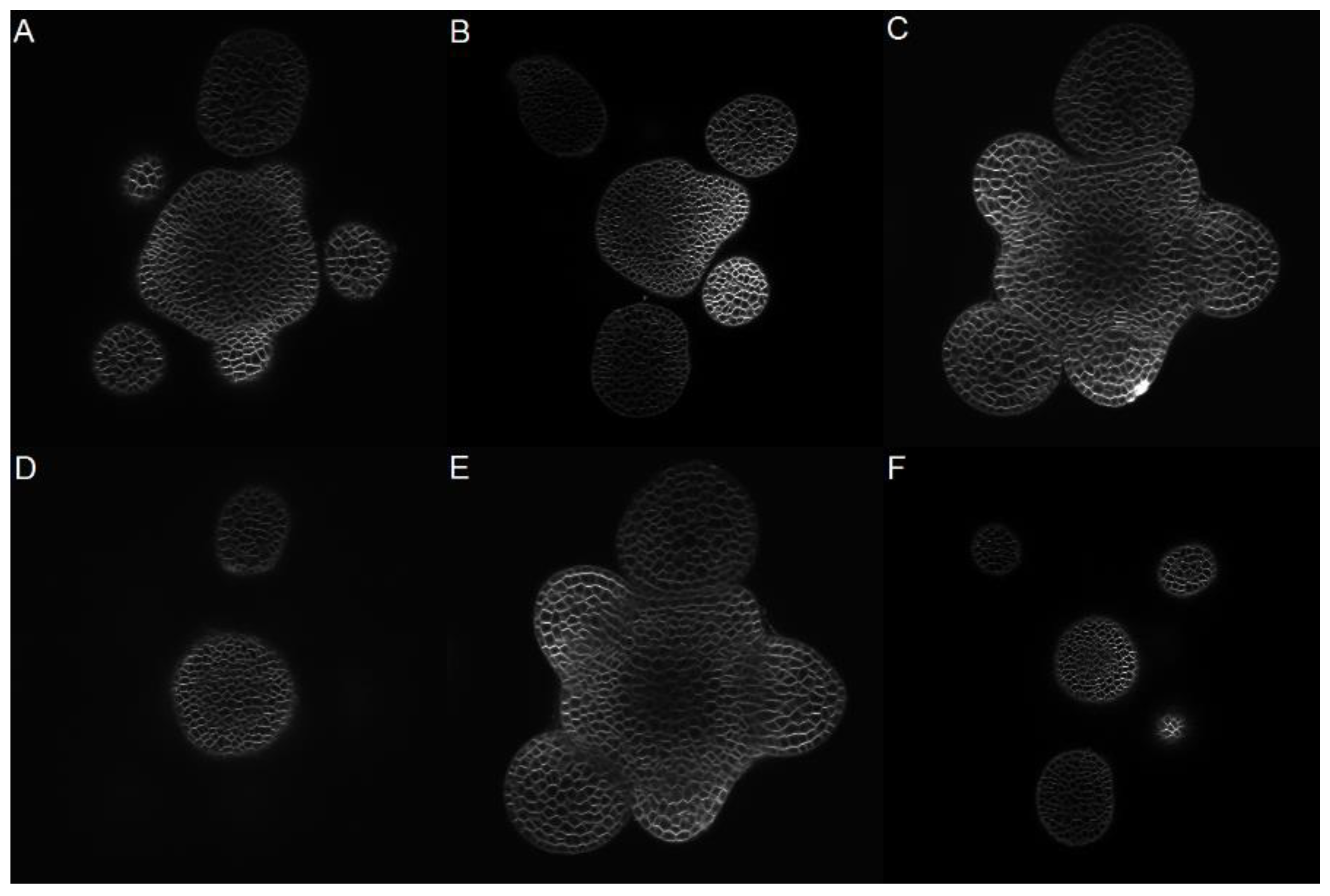
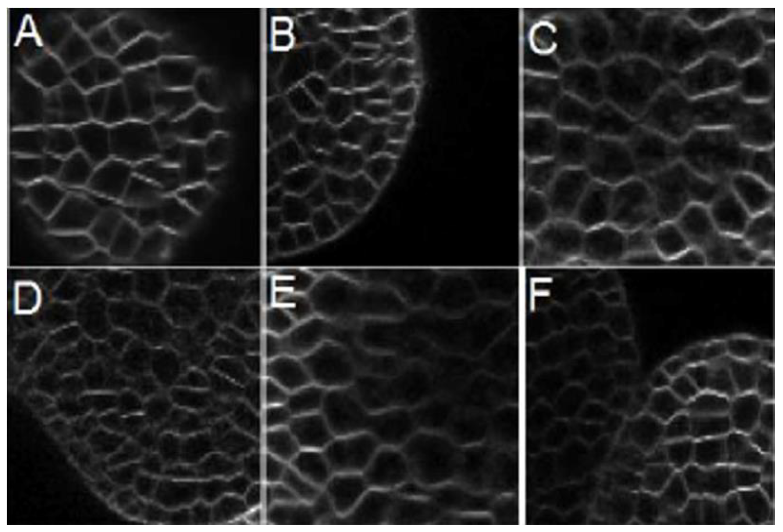
The cells found in the SAM are an example of irregularly shaped, clustered cells (Figure 1). The shapes of the cells are determined by semi-rigid cell walls that surround and join tightly to their neighbors. Cells join to a varying number of neighbors with their common boundary to define individual wall segments. Therefore, these individual wall segments can contribute in different proportions to the total perimeter of a cell, that is, there is no consistent geometrical description of a cell shape. Additionally, the SAM consists of hundreds of overlapped cells, which makes manual segmentation a time-consuming solution. Confocal images of the SAM are characterized by regions of very low contrast and absolute loss of edges when deeper into the meristem. Edges are blurred, discontinuous, sometimes indistinguishable, and the intensity level inside the cells is similar to the image background.

Recent technical advances in microscopy have fostered the development of new image processing techniques. These methods provide useful tools to extract quantitative information from images of biological samples, especially when large data sets must be collected. Several methods have been developed to automate the process of cell identification and segmentation, but most of them assume either that cells have a regular shape or are developed to detect their nuclei.

Molnar et al. [1] discussed the detection of the cell nuclei and their morphology even in high confluence cell cultures with many overlapping cell nuclei. They combined the active contour model “gas of close circles”, which favors circular shapes but also allows slight variations around them, with a new data model. This captures a common property of many microscopic imaging techniques: the intensities of the overlapping nuclei are additive.

Wienert et al. [2] presented a novel contour-based ‘‘minimum-model’’ cell detection and segmentation approach that uses minimal a priori information and detects independent contours of their shape. This approach avoids a segmentation bias with respect to shape features and allows an accurate segmentation (precision 50.908; recall 50.859; validation based on 8000 manually-labeled cells) of a broad spectrum of normal and disease-related morphological features without the requirement of prior training.

Dima et al. [3] found cell edges from fluorescent microscopy images using edge detection and k-means clustering methods. Parvati et al. [4] applied mathematical morphology techniques to derive an edge detection algorithm, including an edge function and a marker-controlled watershed segmentation. This method was applied in medical Magnetic Resonance Imaging (MRI) for brain cell analysis and also in satellite images. The authors reported that the watershed transformation produces good segmentation when markers are used on masks, even if they contain irregularities.

Jung et al. [5] proposed a fully automated watershed-based nuclei segmentation technique. Using the h-minima transformation to identify each candidate nucleus, they found the optimal h value by comparing the distortion between the segmented image and the proposed synthetic model. Dorini et al. [6] proposed a novel method to segment the nucleus and cytoplasm of white blood cells (WBC). They employed simple morphological operators and explore the scale and space properties of a switching operator to improve the accuracy of the segmentation.

Dimopoulos et al. [7] developed a graph cut segmentation that takes into account cell boundary information by means of directional cross-correlation, and automatically incorporates spatial constraints. Cheng et al. [8] suggested an automatic technique to segment cell nuclei in fluorescence microscopy images, using shape markers and marking functions. The method begins with an initial segmentation of nuclei, using active contours without edges. Then, a marker-controlled watershed algorithm is applied with a new marking function capable of accurately separating clustered nuclei. An adaptive h-minima transformation is applied iteratively; then, images are binarized, and a distance transformation is used before the watershed transformation. Singh et al. [9] presented a survey of all the actual division approaches used to divide a picture into non-convergent premises with the ultimate goal that each area is homogeneous, as well as the union of two not nearby districts.

Several techniques can be applied for the automatic or semi-automatic segmentation of Shoot Apical Meristem cells in confocal microscopy images, including a level set algorithm by Liu et al. [10], watershed by Fernandez et al. [11] and Jung et al. [5], and balloons by Federici et al. [12]. However, their methods are not fully automatic, given that several parameters must be fixed beforehand. Stegmaier et al. [13] proposed a development that consists of a conservative super-voxel generation method followed by super voxel agglomeration based on local signal properties and a post-processing step to fix under-segmentation errors using a Convolutional Neural Network.

Several attempts have been made to provide optimal segmentation procedures, but the problem has not been completely solved yet, as image segmentation is, most of the time, an ill-posed problem without a clear unique solution. Most automated-cell segmentation methods need several parameter values to be fixed beforehand in order to get the best results. This process is time-consuming because segmentation must be repeated with each new value, and variations in the image quality must be tackled. Liu et al. [10] are the only authors who propose an automated method to tune a segmentation procedure, but this optimization is based on an approximation between the expected area of the cells and the area of the resulting objects. Thus, it requires previous knowledge.

Rojas et al. [14] introduced a meristem segmentation method based on mathematical morphology, which requires three parameters to be tuned. This segmentation algorithm produces as output a binary image as a function of the variation of three parameters, where a grey level represents the object of interest and another one the background. The automated optimization procedure, proposed by Rojas et al. [15], is employed to tune the segmentation. The technique, called Parametric Segmentation Tuning (PST), is an iterative process that finds the best parameters by comparing the segmented images obtained by successive variations of the parameters. The meristem segmentation technique is extended here and compared with the methods of Liu et al. [10] and Federici et al. [12]. The comparison showed that our procedure led to a significant improvement of the segmentation results.

2. Materials and Methods

2.1. Technical Specifications of the Image Stack

Ten stems wild-type Arabidopsis inflorescence stems (Col0 ecotype) were dissected to expose the SAM, which is normally concealed by the developing floral buds. Field work was not involved, and all samples grew under cabinets with controlled environment in the laboratory, using seeds collected from laboratory-grown plants, obtained originally from the Nottingham Arabidopsis Stock Center (http://arabidopsis.info).

All the work involving plant growth and genetic modification was carried out under the regulations and inspection of the UK Health and Safety Executive. Cell membranes were stained by submerging the structure in a 66 ng/mL aqueous solution of FM4-64 (Life Technologies) for one minute. SAM was imaged using a Zeiss 710 confocal system with an Observer Z1 microscope stand and an Achroplan 40×/0.8 W long working distance water-dipping objective.

Excitation was provided at 488 nm (3% power) and emission collected between 605 and 695 nm using a pinhole of 54 µm (1 Airy unit). Ten stacks of 102 images on average were acquired with a xy resolution of 512 × 512 pixels (pixel size 0.52 µm²) and z-spacing of 0.52 µm. Gain and offset were optimized to give the best contrast between stained cell walls and unstained cytoplasm as assessed by eye.

Each stack is sufficiently representative to make an analysis and generalize the segmentation process as it contains most of the characteristic issues that affect this type of images (blurriness, diffuse contours). Figure 1 shows three images from two of the stacks, randomly chosen at different depths. From each one of these images, a subsection of size 322 × 320 pixels was chosen to test the methods and segmented by hand to obtain six manually annotated ground truth images.

2.2. Segmentation Algorithm

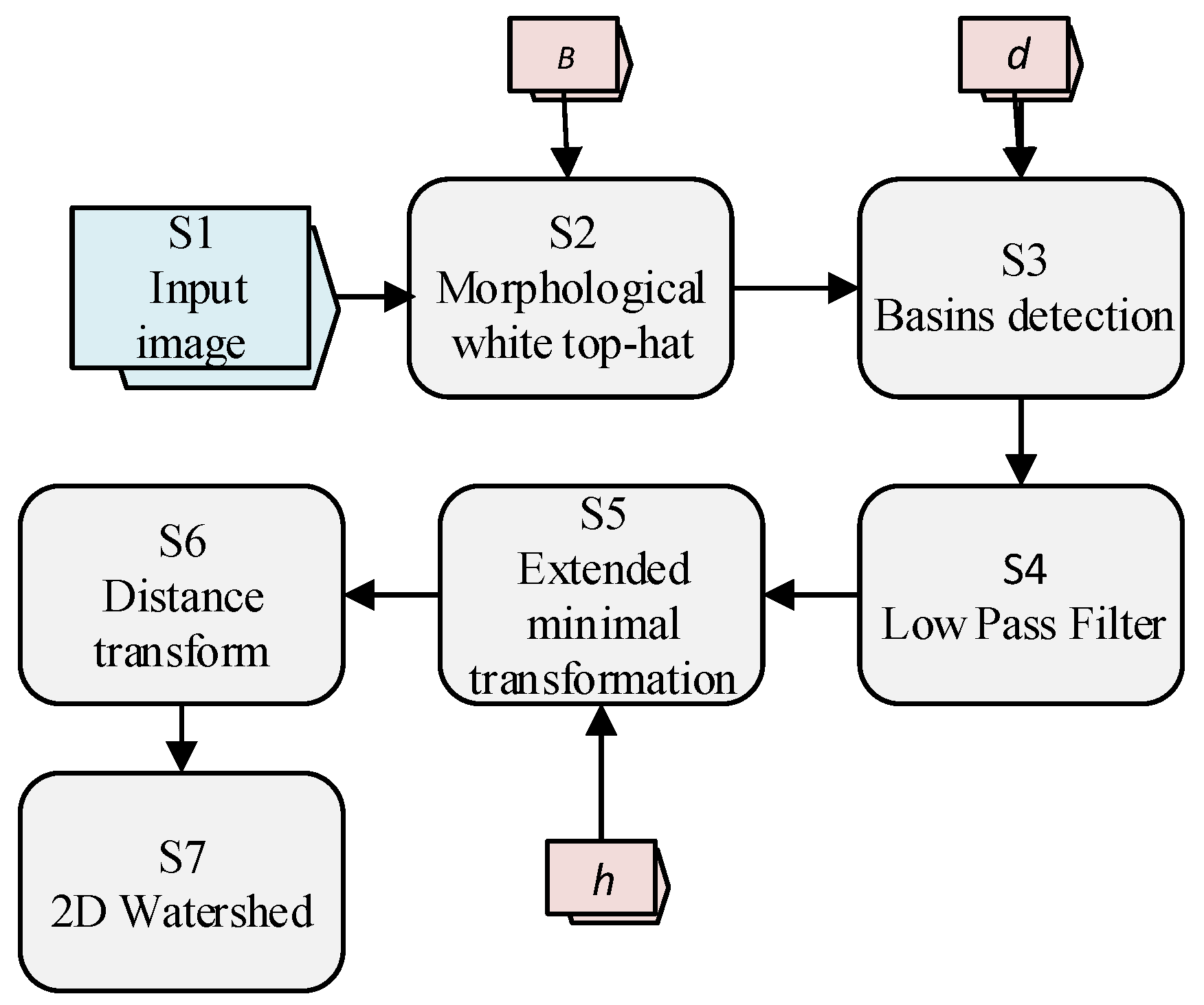
Rojas et al. [14,15] introduced an automatic tuning technique for segmenting diatom images, which is used here to find the best values of the proposed segmentation technique. As shown in Figure 2, three parameters ${\overrightarrow{p}}_n=\left[B,h,d\right]$ must be set to find the best segmentation. For each variation of one of the parameters, a segmented image is obtained. For the sake of simplicity, we call ${\overrightarrow{p}}_n$ to the image obtained with a certain set of parameter values and ${\overrightarrow{p}}_{n+1}$ to a neighboring image in the parameter space, obtained by the variation of one of the parameters.

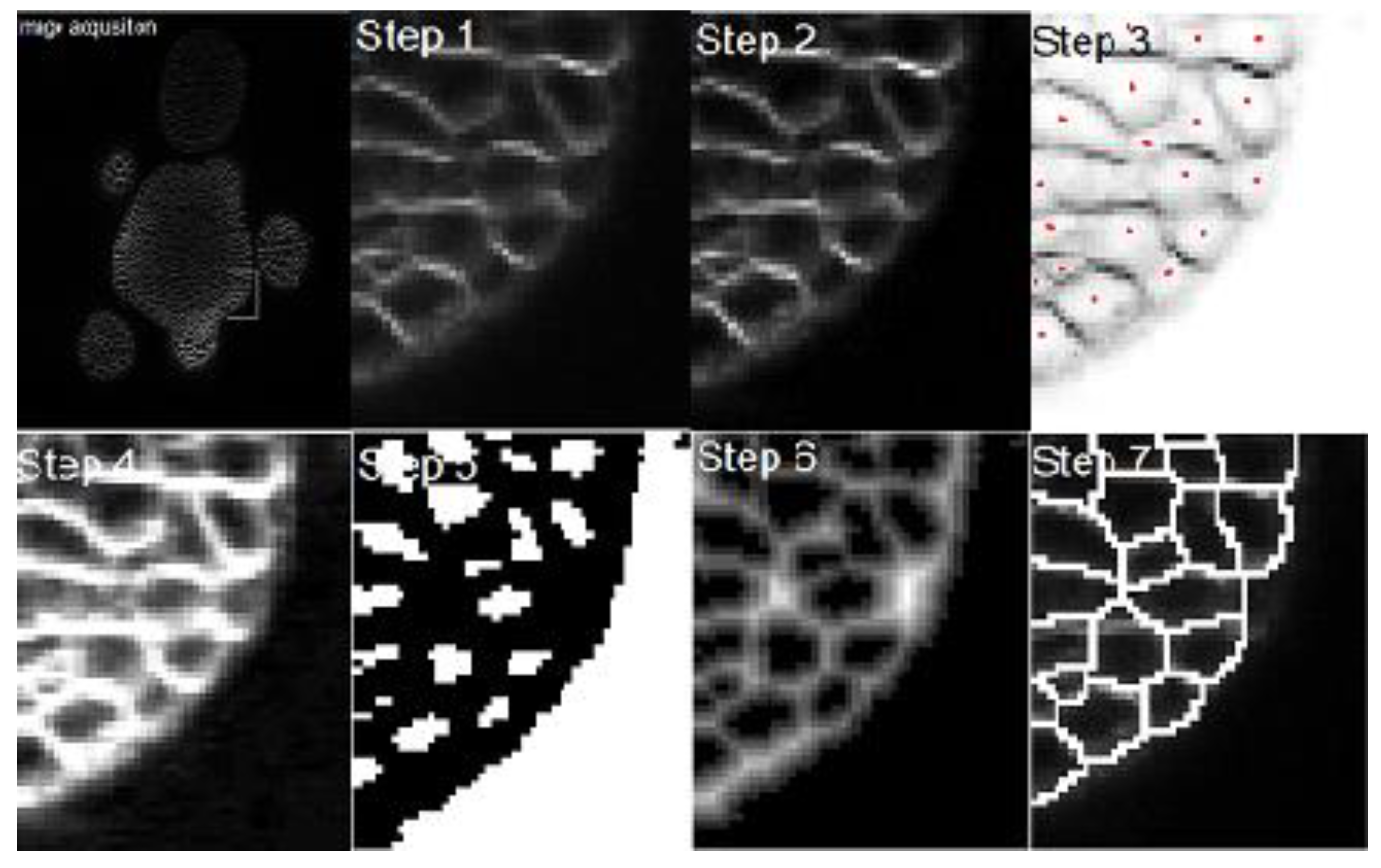
To segment the meristem stacks, a method of seven steps is proposed, as shown in Figure 2 and Figure 3. First, a white top-hat transform (e.g., Beucher [16] and Vincent [17]) is employed to highlight the edges of the cells, in particular those in low contrast regions (Figure 3—Step 2). By applying this transform, the bright details of the image are highlighted on a dark background. To get a good result, the appropriate size of the structuring element B, i.e., the first parameter of the method, is fixed as explained in Section 2.3.

Then, to identify each candidate cell, a seed or mark must be placed in each of them. In the images, the cells are identified as black regions surrounded by bright walls. If the image is seen as an orographic system, where the altitude of each point is given by the intensity of the pixel, then, each cell can be identified by finding its local minimum. In this way, seeds are found across the basins in the images, as defined by Vincent [18] (Figure 2 and Figure 3—Step 3). The depth of the basin is given by d and ideally, a single seed should be found for each cell. However, depending on the chosen value of depth d, one seed can be shared amongst several cells (if d is too big), or one cell may contain several seeds (if d is too small). To solve this problem, the optimal depth d is found, as explained in Section 2.3. Since more than one basin can still appear inside a cell, a steerable Gaussian filter is used to remove the false seeds, as shown in Step 4 of Figure 2 and Figure 3. In Step 5 (Figure 2 and Figure 3), seeds are finally determined by computing iteratively the extended-minima transform of height h. As cells have irregular shapes and their edges are not detectable by classical geometry, they are identified by the region of minimum intensity. Thus, by varying h, it is possible to find the regions that contain the local minima of the image. In the ideal case, a single local minimum contained within each cell is obtained.

Then, the distance transform by Vincent et al. [19] is used as a model of probability distribution and applied in Step 6 (Figure 2 and Figure 3). The distribution around the minimum determines the zone of influence of each cell, which corresponds to the internal region bordered by the cell edges. Once the zone of influence is identified, the watershed transform is applied, and the area of each cell is found in Step 7 (Figure 2 and Figure 3).

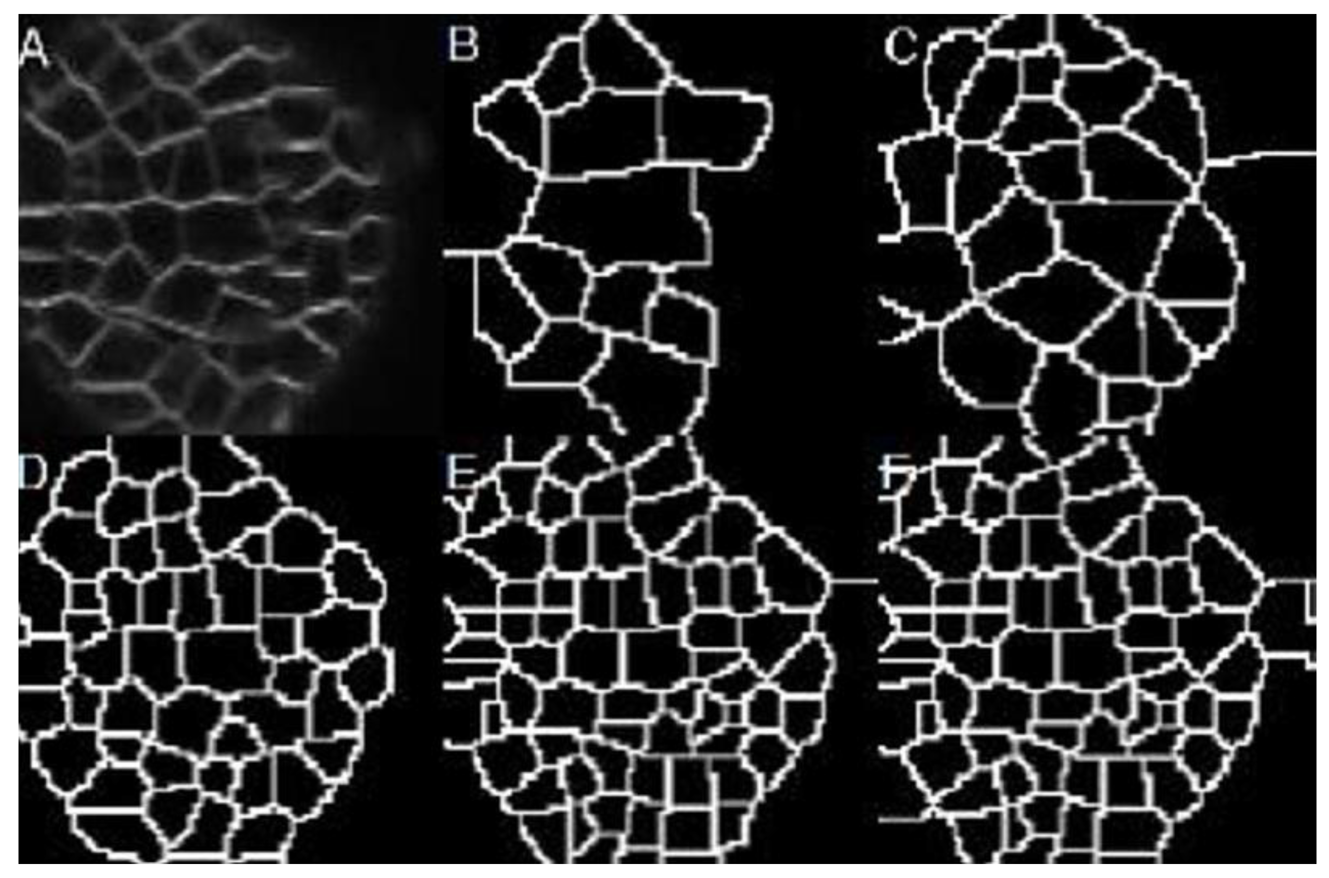
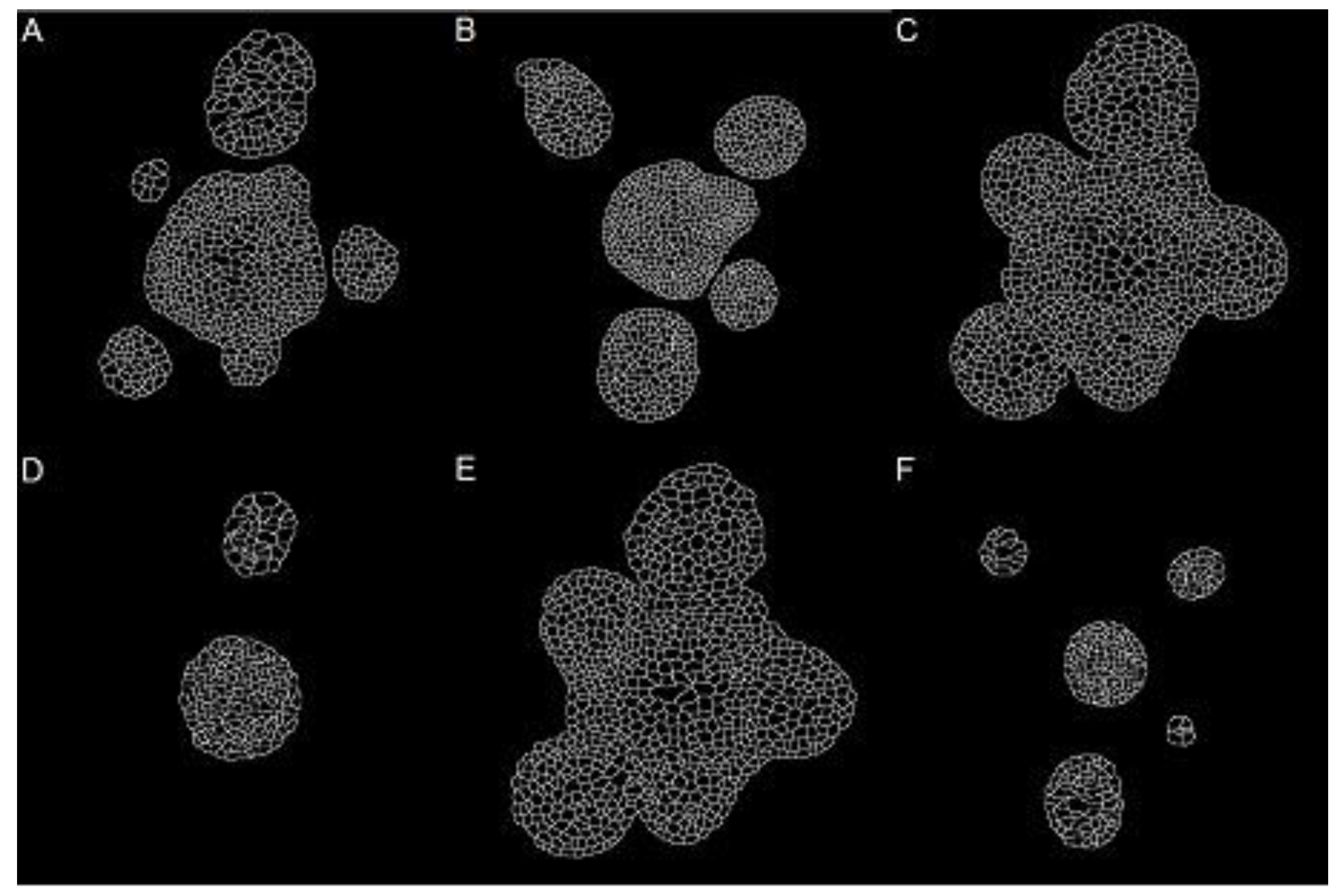
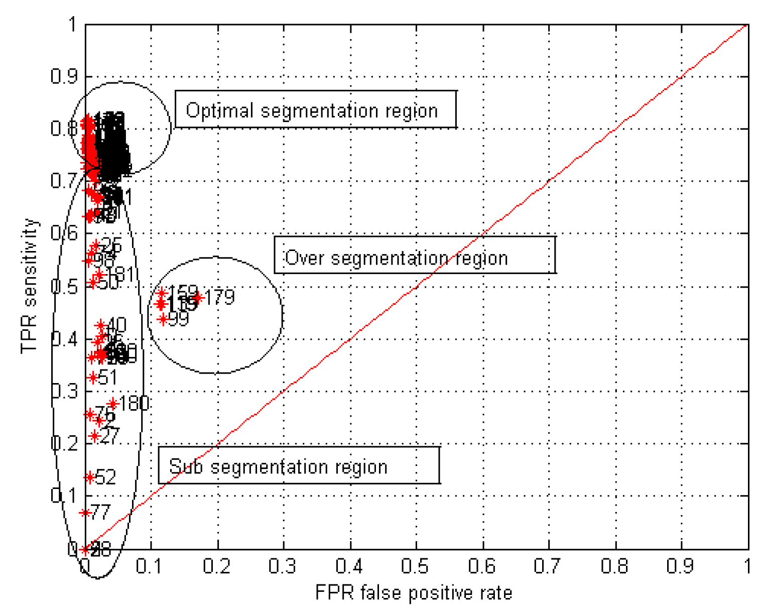
As shown in Figure 4, varying a parameter within a range of values in the segmentation method produces a move from under-segmented images to over-segmented ones that passes through an intermediate value, where the best possible result is obtained. Changes between under-segmented and over-segmented images are more abrupt compared to those produced between the images closer to the optimal result. This behavior is expected because the optimal result seeks to get closer to what is actually seen in the original image. In other words, if two consecutive under-segmented images are compared, the second one will be more segmented than the first one. Thus, if two consecutive under-segmented images are matched, the first will be less sub-segmented than the next. Assuming that the first image is the ground truth image, there will be zero false negatives and a high number of false positives. Similarly, if two consecutive over-segmented images are compared, the second one will be more over-segmented than the first one. In this case, if it is assumed again that the first image is the ground truth, the second one will have zero false negatives and a high number of false positives. If the segmented images are close to the optimal result, the variation between them will be minimal and the number of false positives will be low. This observation was used by Rojas et al. [15] to develop their tuning technique. Since the same observation is also true in the meristem images, the PST was used here to fine-tune the segmentation algorithm. The ground-truth images obtained by hand were only used to validate the results. To validate the method, the binary images obtained were compared with the ground truth using the Jaccard index.

2.3. Overview of the Parametric Segmenting Tuning Technique (PST)

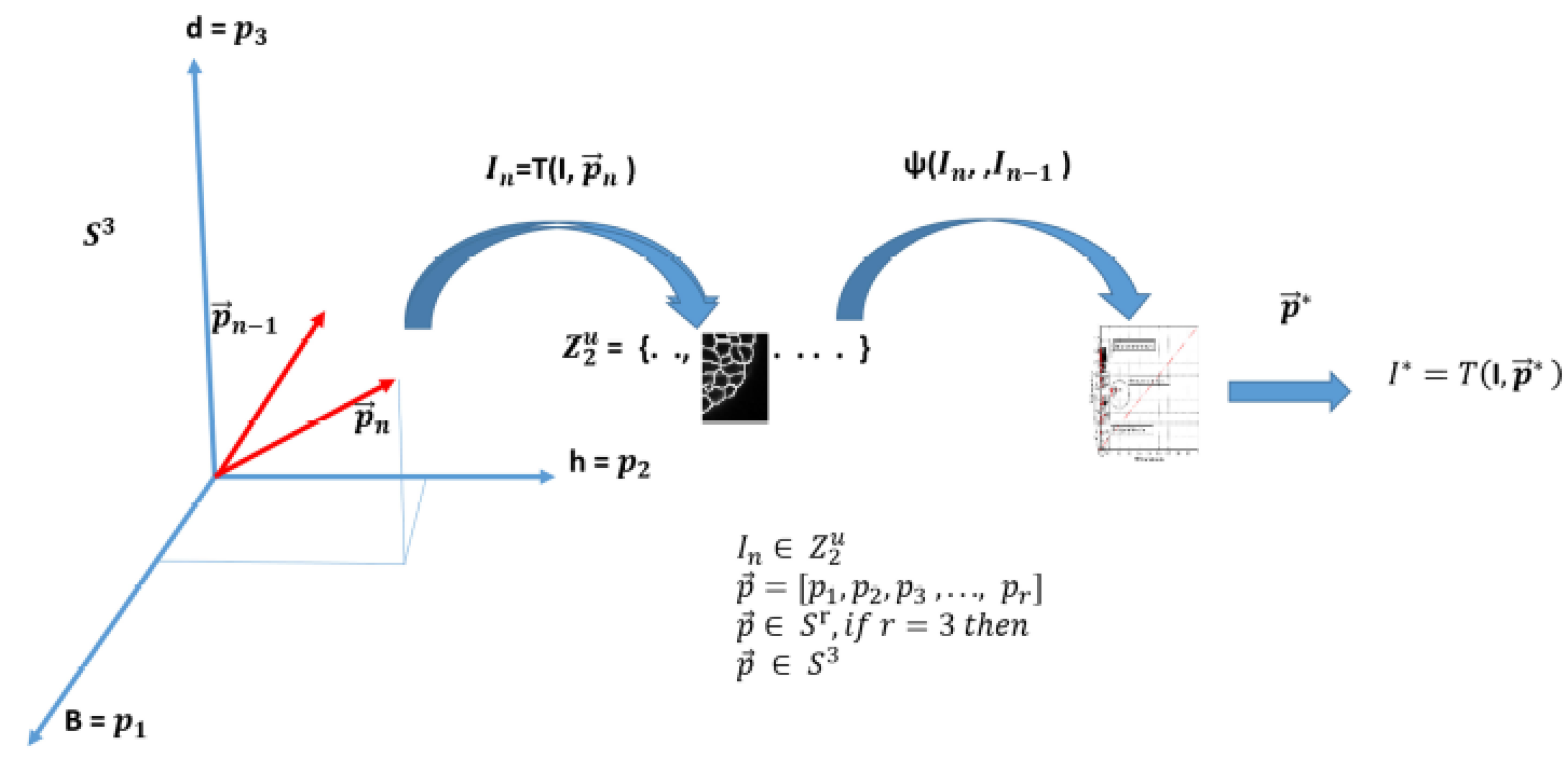
The PST technique is briefly described here and employed to tune the segmentation algorithm. An image $I$ of size $N\times M$, where $N$ and $M$ are the width and height of the image, respectively, may be represented as a vector $\alpha$ of size $u=N\times M$. Let $T\left(I,\overrightarrow{p}\right)$ represent the transformation of an image I into a binary one as a result of a segmentation algorithm, given a certain number $r$ of parameters $p$, where a grey level represents the object of interest and another one the background.

Therefore, an $r$-dimensional solution space $P^r\subseteq R^r$ generated by the transformation $T\left(I,\overrightarrow{p}\right)$ can be defined, where each coordinate is given by a parameter and each point of the space represents a binary image. Considering image segmentation as an optimization problem, the best solution can be found by maximising a similarity function $\Psi$ in $P^r$, or minimising a distance function.

The object function is defined as: $\Psi :Z_2^u\times Z_2^u⟶R$, where $\Psi$ is an indicator associated to each pair of neighbor images of $Z_2^u\times Z_2^u$. Each binary image $I_n$ is an element, in the space of possible solutions $P^r\subseteq R^r$, generated by the transformation $T\left(I,{\overrightarrow{p}}_n\right),$ as shown in Figure 5.

The decision criterion consists of finding the set of images with the highest associated index (maximization problem), or the lowest associated distance (minimization problem).

Table 1. Definition of the similarity and distance indices used for tuning the Parametric Segmentation Tuning (PST).

Index	Definition	Mathematical Expression
Sensitivity	It represents a relationship between the True Positive Rate (TPR) and the False Positive Rate (FPR). It varies between zero and one, being minimal when the FPR is zero and maximum when the TPR is one.	${\Psi }_{IS}\left(\alpha ,\beta \right)=0.5\left(1+TPR-FPR\right)$
Coverage	It compares the reference and segmented sets α and β, measuring the one-to-one correspondence between the pixels of both sets.	${\Psi }_{IC}\left(\alpha ,\beta \right)=\frac{2\alpha ·{\beta }^t}{\Vert \alpha \Vert + \Vert \beta \Vert }$
Minimum Distance	Minimum distance in the ROC space between the optimum segmentation point (0.1) and the one located in (FPR, TPR).	${\Psi }_{dmin}\left(\alpha ,\beta \right)=\sqrt{1-TP{R}^2+FP{R}^2}$
Collinearity	It measures how well two sets of points of the compared images α and β match each other. It varies between 0 and 1, being zero if the sets of points are orthogonal and one if they coincide, i.e. they are collinear.	${\Psi }_{ICo}\left(\alpha ,\beta \right)=\lambda =\frac{\alpha ·{\beta }^t}{\Vert \alpha \Vert · \Vert \beta \Vert }$

presents the four indices used here and explained in [15]: Sensitivity, Coverage, Minimum Distance and Co-linearity. The sensitivity and Minimum Distance Index relate the True Positive Rate (TPR) and the False Positive Rate (FPR). The relation between the TPR and the FPR is known as ROC space (Receiver Operating Characteristic).

Let the binary set $Z_2=\left\{0,1\right\}$ be the binary space $u$-dimensional $Z_2^u=Z_2\times Z_2\times \dots \times Z_2$ $u$-times.

An element $\alpha$ (image) of $Z_2^u$ is an u-upla formed by $Z_2$ elements. Thus, $\alpha =\left({\alpha }_1,{\alpha }_1,\dots {\alpha }_u\right)$, with ${\alpha }_i\in Z_2$, that is, $Z_2^u=\left\{\alpha =\left({\alpha }_1,{\alpha }_1,\dots {\alpha }_u\right),\vee ,\alpha \in Z_2\times Z_2\times \dots \times Z_2\wedge {\alpha }_i\in Z_2\right\}$.

In other words, the optimal segmentation parameters are obtained by finding the best index value between each pair of neighboring images, which can be expressed mathematically as follows:

$$\begin{array}{c}{\overrightarrow{p}}^{\ast } =\arg \{optimum({\Psi }_{\left[·\right]}\left(I_n,I_{n-1})\right)\}\\ \mathrm{Subject} \mathrm{to}: I_n\in Z_2^u\end{array}$$

(1)

Therefore, the best solution, noted by an asterisk ${\overrightarrow{p}}^{\ast }=\left[B^{\ast },h^{\ast },d^{\ast }\right]$, can be found in Figure 5 and Figure 6, by sweeping the solution space and evaluating a similarity function between each pair of binary neighbor images $I_n=T\left(I,{\overrightarrow{p}}_n\right)$ and $I_{n-1}=T\left(I,{\overrightarrow{p}}_{n-1}\right)$. These images are the result of the segmentation algorithm $T\left(I,\overrightarrow{p}\right)$ explained in Section 2.1.

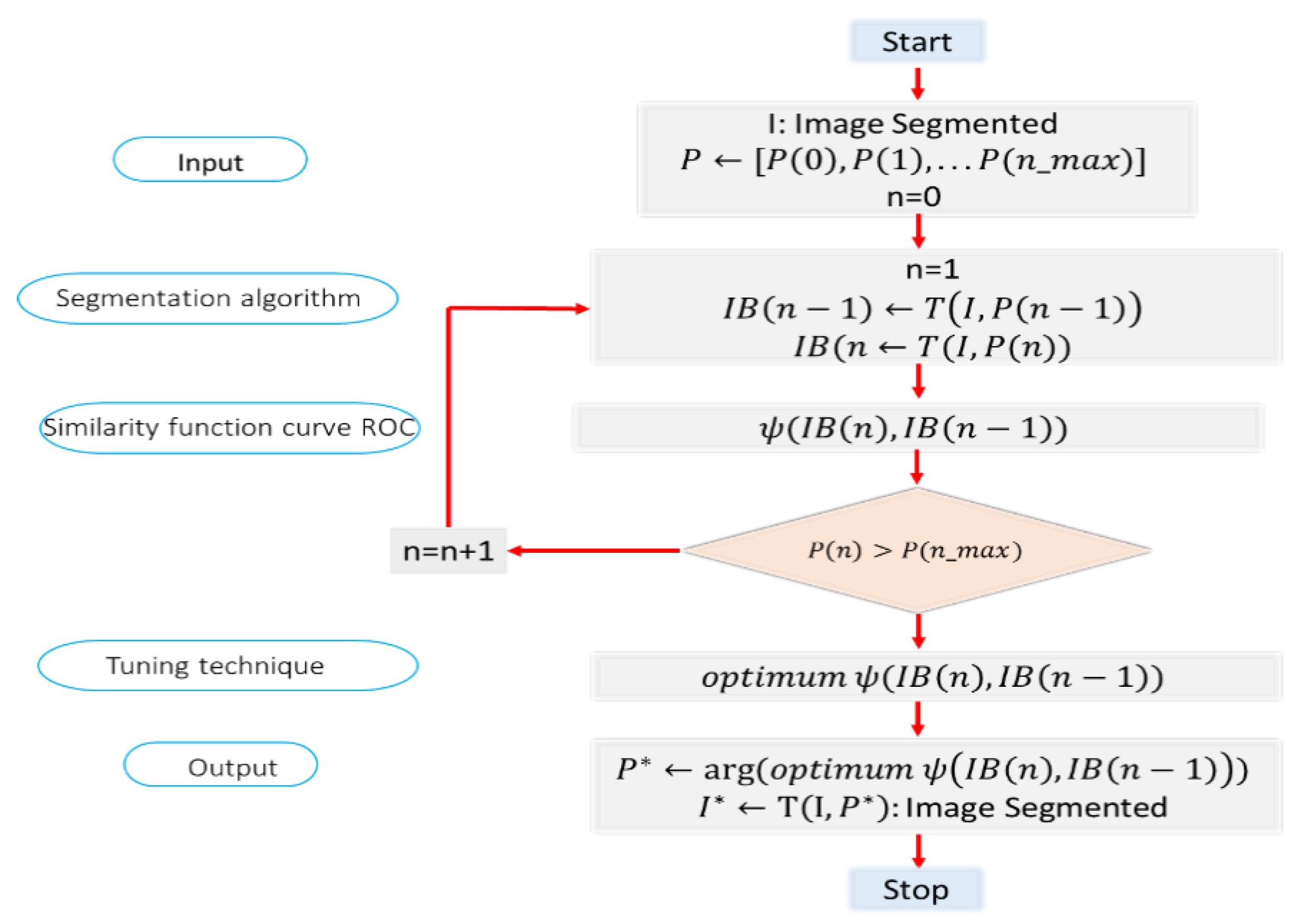
Since there are three parameters to be tuned, the PST Algorithm 1 can be implemented with the following pseudo-code:

Alogrithm 1: Parametric Segmenting Tuning Technique (PST)

1: Input: I original image 2: Output: optimal segmented image 3: $I_n$: Image segmented in step n 4: $B,h,d$ Parameters to be tuned 5: $B^{\ast },h^{\ast },d^{\ast }$ Optimal parameters 6: $n=1$ 7: $I_{n-1}=White\_Image$ 8: $for\left(B=B_{min};B\le B_{max}B++\right)$ 9:   $for\left(h=h_{min};h\le h_{max}h++\right)$ 10:     $for\left(d=d_{min};d\le d_{max}h++\right)$ 11:     $\{$ 12:       $I_n=segmentation\left(B,h,d\right)$ 13:       $if\left(\psi \left(I_n,I_{n-1}\right)isoptimun\right)then{B}^{\ast }=B,h^{\ast }=h,d^{\ast }=d$ 14:       $previous{I}_{n-1}=I_n$ 15:     $\}$ 16: $Optimal\_Image=segmentation\left(B^{\ast },h^{\ast },d^{\ast }\right)$

This algorithm is slow, but it allows finding the optimal segmentation parameters. It is possible to build more efficient algorithms to obtain the best parameters, although this objective is beyond the scope of this work. However, a faster method to get the approximate parameters consisted in sweeping one parameter (B), while the other two remain fixed until finding the value (B) that allows obtaining the best index. Then, another parameter (h) is swept, while the other two remain fixed (B with the best value found) looking also for the best value. This process is applied to all three parameters. This approach is much faster and was used to find the optimal values of the segmentation method.

3. Experiments, Results, and Discussion

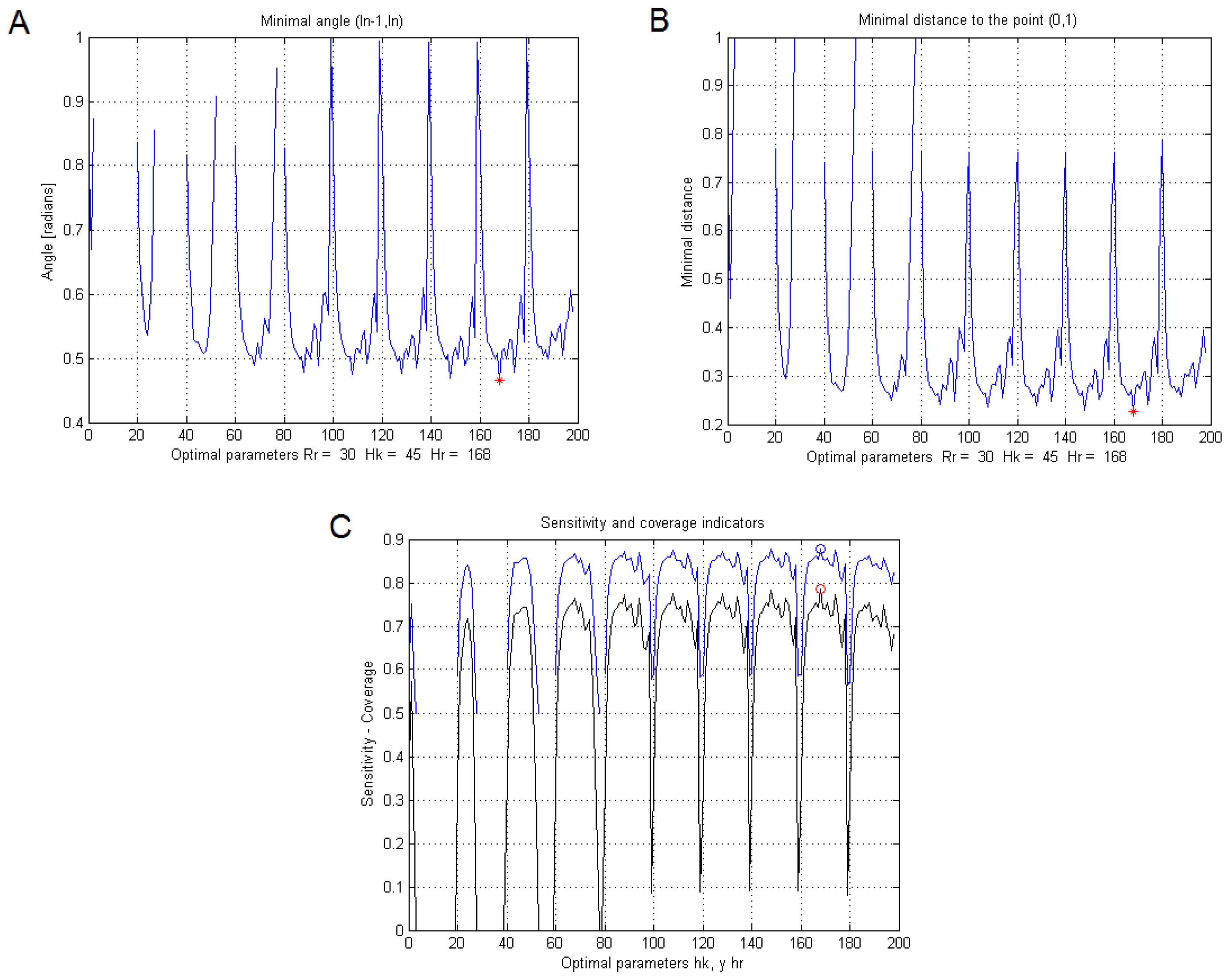
Figure 7 shows the results of the segmentation. The four similarity indices shown in Table 1 were used to find the optimal parameters and determine the most efficient. Figure 8 shows the similarity curves obtained by each index, with ten different values of d, while modifying h and keeping B constant. Figure 8A shows the collinearity index, Figure 8B the minimum distance to the point index (0.1) and Figure 8C the coverage and sensitivity indices, where the maximum values of each iteration in d (horizontal axis) are the arguments of h.

From those iterations, the algorithm chooses the one with the lowest error and the highest match. Figure 9 shows the ROC curve and the trend towards the point (0,1) between the two neighbour segmented images. Points are located in the upper left part of the 45° line. The parameters vary from left to right, passing by a point in which high true positive and low false positive rates are found. This point is the minimum distance to (0,1) in the ROC curve, which means that the best pair of segmented images has been found.

Table 2. Parameter values and optimal similarity indices obtained with the proposed method for each image in Figure 7.

Images	B	d	h	Sensitivity Index	Coverage Index	Minimum Distance Index	Co-linearity Index
A	30	10	4	0.856	0.737	0.273	42.48
B	30	10	3	0.852	0.736	0.279	42.52
C	30	10	4	0.855	0.742	0.266	42.01
D	30	20	6	0.846	0.729	0.331	44.78
E	30	10	4	0.841	0.717	0.293	44.13
F	30	10	4	0.835	0.673	0.342	45.68

shows the indices and optimal values found for the parameters of the segmentation method, for each image in Figure 7. The same optimal parameters were found with each index. Therefore, the computational load was used as the only criterion to choose sensitivity as the best tuning index.

To validate the method, the binary images obtained were compared with the ground truth using the Jaccard index. As shown in

Table 3. Jaccard index obtained between the results of the proposed method and the ground truth images.

Images/Ground-Truth	B	d	h	Jaccard Index %
A	30	10	4	94.00
B	30	10	3	90.09
C	30	10	4	93.44
D	30	20	6	96.51
E	30	10	4	96.77
F	30	10	4	96.20

, the Jaccard index is higher than 90, which shows the quality of the obtained segmentation.

3.1. Comparison with Level Set Algorithm and Balloon Segmentation Technique

Six sub-images from the stacks were randomly selected and segmented using all the three methods. The results obtained with the available free methods depend on the value of a parameter chosen by the user, in addition to delivering no binary segmented image itself, but rather the highlighted contours of the cells at grey levels. Therefore, the cells found were marked and numbered for different values of the input parameters. The true and false positive percentages were then obtained. 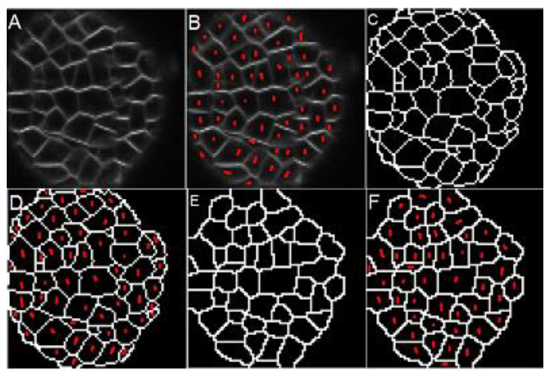Figure 10A illustrates an example of the result obtained with the proposed method in a sub-image from Figure 1. Figure 10B shows the fifty cells identified by hand. Figure 10C shows the ground-truth, and Figure 10D presents the ground-truth overlapping the original image. Figure 10E,F expose the result obtained with the proposed method: 47 cells were identified with a non-success error of 6% compared with the ground-truth.

3.2. Comparison with the Level Set Algorithm Technique

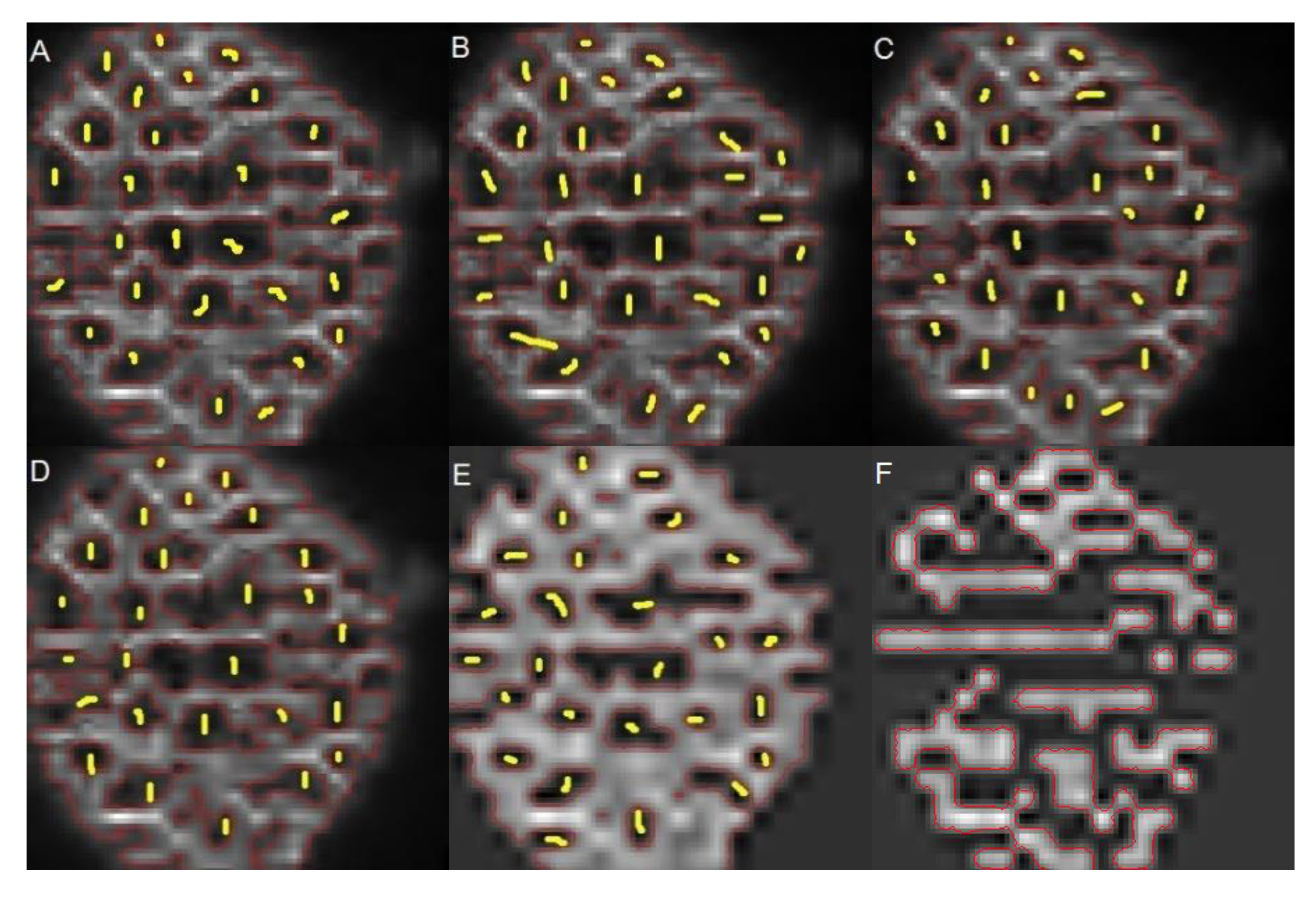
The algorithm proposed by Liu et al. (Liu, Yadav, Chowdhury, & Reddy, 2010) adapts the region-based energy model, known as the Chan-Vese Level Set Model for segmentation. Figure 11 shows a sequence of four different results obtained by modifying the model level $h$.

The segmented images were compared to the original ones and to the ground-truth. For each level of segmentation, cells that matched the ground-truth were listed. In Figure 11A ($h=1$), Figure 11B (h = 3) and Figure 11 ($h=100)$, it is possible to see that the technique estimates the cells edges. However, when the threshold level increases, the algorithm begins to detect high intensity regions instead, as shown in Figure 11D ($h=150$), thus, cells are not identified.

Table 4. Results obtained with the proposed method and the level set algorithm for different values of level h.

Method	Level h	Found Cells	Failures [%]
Ground-truth	-	50	0
PST	-	47	6
	1	26	48
	3	30	40
	5	29	42
	7	29	42
	10	27	46
Level set	12	28	44
	20	26	48
	35	28	44
	50	29	42
	100	26	48
	150	0	100
	200	0	100

summarizes the results obtained by comparing the ground-truth image, the one segmented by the proposed method, and those obtained with the level set algorithm. The maximum success rate was reached at level 3, where a failure rate of 40% was obtained, which is high compared with the 6% obtained with our method.

3.3. Comparison with the Balloon Segmentation for Multicellular Images—BSMI Technique

The technique described by Federici et al. (Federici, Dupuy, Laplaze, Heisler, & Haaeloff, 2012) uses a physical balloon inflation algorithm to detect cellular architectures from the cell wall segmentation in microscopy images. This method extracts information about the cellular morphology and determines which cells are in contact with each other. The stages of the process are automatic. However, manual changes can be made at each step.

Prior to segmentation, this technique uses a pre-processing step. Then, in the first stage, the Watershed Transform is applied to find the edges of the cellular tissue to be segmented. In the second stage, the seeds used to recognize each cell are found, manually or automatically, through a sampling algorithm based on the “path” between two points to determine if both are inside the same cell. If the foregoing is true, one of them is removed. This decision is based on the product h*l, where h is the highest intensity along the path and l the distance between points. If there is a small relation, the point belongs to the cell, but if there is a large one, some cells cannot be detected. 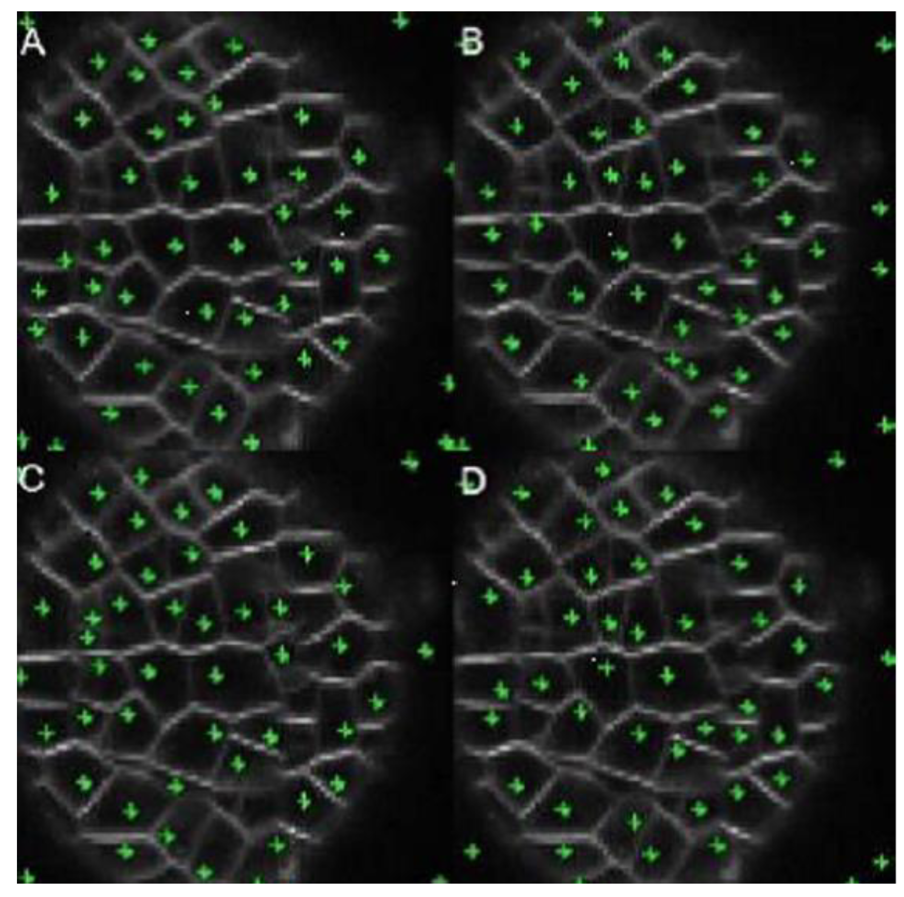Figure 12 shows a sequence of four images segmented by the BSMI technique with increasing values of the product h*l. This technique identifies regions with low-intensity levels, surrounded by pixels with higher levels to detect and locate the central parts of each region. The sequence of images shows that, in some areas, the centers are adequately located. However, some of them are outside the region of interest, hence producing false positives in the background.

Table 5. Results obtained with the proposed method and the BSMI technique.

Method	BSMI	Found Centers	Found Cells	Failures [%]
Ground-truth	-	-	50	0
PST	-	-	47	6
	7	47	40	20
	10	45	39	22
	15	49	44	12
	20	50	42	16
	25	46	39	22
	30	46	40	20
Balloon	50	47	39	22
Technique
	100	46	41	18
	120	42	37	26
	300	48	41	18
	500	47	41	18
	5000	45	40	20

summarizes the results obtained by comparing the ground-truth image, the one segmented by the proposed method and those obtained with BSMI technique. The maximum success rate was reached for h*l = 15, where the failure rate was 12%, compared with the 6% obtained with our method.

Table 6. Results obtained with the meristem segmentation methods.

Sub-Images	Ground-Truth	Proposed Method		Level Set Algorithm			BSMI
	Cells	Found Cells	Failure [%]	Level Set	Found Cells	Failure [%]	h*l	Accurate Cells	Failure [%]
A	50	47	6.00	3	30	40.00	15	44	12.00
B	55	50	9.09	7	32	41.82	10	41	25.45
C	61	57	6.56	7	20	67.21	30	53	13.11
D	86	83	3.49	1	44	48.84	10	69	19.77
E	62	60	3.23	10	15	75.81	300	60	3.23
F	79	76	3.80	7	22	72.15	25	69	12.66

Summarizes the number of cells found with the different methods in the six sub-images shown in Figure 13, which were taken from each image in Figure 1, using the best parameters found by hand in the level set and BSMI techniques. Results show that the proposed method has better performance, losing 9.09% of the cells in the worst case.

4. Conclusions

A method for the segmentation of meristem cells was introduced in this paper, based primarily on mathematical morphology techniques. The proposed method requires the adjustment of three parameters. For its automatic optimization, the technique called Parametric Segmentation Tuning was employed. In the PST, optimal parameter values are obtained through an iterative process. In this way, automatic segmentation of microscopy images of the shoot apical meristem, containing irregularly shaped cells with variable contrast, is achieved with improved reliability. The PST technique can employ a variety of similarity functions or distances. When these functions are optimized, they allow for estimating the best parameters of the segmentation algorithm. The indices tested produced the same results, thus finding that the sensitivity index is better thanks to its lower computational cost.

Experimental results showed that the proposed method is effective, eliminates false objects produced by local minima, and correctly identifies cells. This technique requires no geometrical information to obtain the best segmentation and could be applied with any other state of the art meristem segmentation technique, where several parameters must be adjusted by hand. When validating with the ground-truth images, it is concluded that the proposed segmentation technique is accurate in at least 90% of the cases, and better results are obtained than those of techniques based on level set algorithm and balloon segmentation techniques.