Article

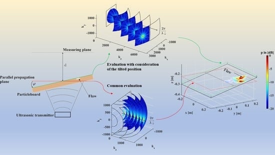
Flaw Detection on a Tilted Particleboard by Use of the Spec-Radiation Method

by
Andreas Sebastian Schmelt
* and
Jens Twiefel
*
Institute of Dynamic and Vibration Research, Leibniz University of Hannover, 30823 Garbsen, Germany
*
Authors to whom correspondence should be addressed.
Appl. Sci. 2020, 10(23), 8513; https://doi.org/10.3390/app10238513
Submission received: 5 November 2020 / Revised: 22 November 2020 / Accepted: 25 November 2020 / Published: 28 November 2020
(This article belongs to the Special Issue Holography in Acoustics and Ultrasonics)

Abstract

:
Herein, we present a novel approach to the spec-radiation method (a method of acoustical holography) for determining the sound distribution on a tilted particleboard by calculating a single plane and rotation in the frequency domain. The tilted particleboard allows testing without standing waves between the transmitter and the particleboard. This eliminates the need to evaluate several parallel planes and to search for values belonging to the tilted particleboard. The numerical requirements can be optimally exploited through a combination with a flaw detectability enhancement method. The results are supported by experiments on a wooden particleboard with flaw imitations. Finally, we showed, through a comparison with the usual procedure of identifying a flaw (calculating many parallel planes and then selecting the data belonging to the tilted plane), that the calculation of the tilted plane is up to 98.5% faster and improves the detectability of flaws in a tilted particleboard.

Graphical Abstract

1. Introduction

Non-destructive ultrasonic testing has been a widely used method for quality assurance since [1] used continuous ultrasonic waves to identify material defects for the first time. In the 1940s, when Firestone developed the first echo material tester based on the reflection principle and Trost designed ultrasonic pliers based on the transmission method, the development of ultrasonic testing was unstoppable [2,3]. Since then, many different methods have been developed, which can be divided into different test arrangements. These include the pulse echo method, in which a receiver and a transmitter or a transmitter that also serves as receiver are located on one side of the test material. The transmitter sends a pulse to the test material via an ambient or contact medium. If there is a difference in acoustic impedance in the test material itself, a reflection or echo is sent back to the transmitter or receiver. Based on the time of flight (ToF) and amplitude of the echo, the location can be determined and conclusions can be drawn about the reflection behavior [4]. Moreover, surface wave testing methods are a large field. Here, a surface wave such as a Lamb wave is generated by a transmitter that is aligned at a certain angle to the test material and recorded by a receiver. This enables the detection of flaws near surfaces or the identification of materials [5]. Another very important method for non-destructive ultrasonic testing is the ultrasonic through transmission technique. Here, a transmitter is located on one side of the test material and a receiver on the other side. If the receiver is moved and the transmitter is stationary, tomographic examinations can be performed. This method is particularly suitable for thick components because, in contrast to the pulse echo method, the sound waves travel through the workpiece only once [6]. These methods allow runtime and intensity measurements to be carried out, also allowing conclusions to be drawn about inclusions and heterogeneities in the material. If one wants to identify air inclusions or the like, one can differentiate according to the type of excitation signal. A broadband excitation leads to high-frequency resonant standing waves in defects, which can be determined from the recorded spectrum [7].
Another excitation method is based on an ultrasonic pulse consisting of a few sinusoidal oscillations. Here, the defect or heterogeneity is evaluated by a change in the phase position or amplitude of the received pulse [8,9]. Ultrasonic testing, in which the transmitter and receiver come into contact with the test material, could lead to high errors in the measurement if the contact force is not controlled [10]. A contact oil is also often used, which causes residues on the surface of the test material [11]. If this is to be avoided, contactless testing is recommended. In this case, the ambient medium plays an important role. In many cases, water is used as the ambient medium due to its fairly well-matching impedance properties [12]. There are, however, materials that must not come into contact with water or other liquid media, because it runs the risk of changing the material’s properties or absorbing the fluid. An example of such a material is wood. For such materials, air is preferred as the ambient medium [13]. However, there is a very large difference in impedance between air and wood, so that a large part of the wave energy is already reflected at the interface between air and wood [14]. In order to counteract this, powerful ultrasonic transducers have been developed in recent years [15] that are able to better combine the impedance between the ultrasonic transducer and the air via innovative matching layers in order to transfer more energy to the air [16]). Thus, it is possible to examine wood-based materials with the through transmission technique and air-coupled ultrasound.
Wood-based materials are once more becoming a popular choice in the civilian population as furniture materials because they are considered a sustainable raw material. The large furniture manufacturers want to meet this demand and, at the same time, to reduce the costs of production, which often works through material savings, and thus ever thinner or less dense particleboards are being used whilst ensuring that the furniture can withstand loads. During the production process of a particleboard, air inclusions and imperfectly glued regions can strongly influence the load capacity [17]. Manufacturers must then test their wood products non-destructively to guarantee the high demands of the furniture industry. The first to deal with the detection of delaminations or flaws in wood-based materials by ToF measurements were [18,19]. In today’s modern particleboard industry, particleboards are tested directly in the running production process. However, due to pressing and gluing, these boards have temperatures of up to 100 C and vapors can still escape, which might damage the receivers [17].
This leaves air-coupled ultrasound as a testing method, with large distances to the particleboard of >100 mm. If a pulse excitation is used, sufficient time must be allowed between one ultrasonic pulse and the next. Otherwise, reflections of the previous ultrasonic pulse between the transmitter and the particleboard or between the particleboard and the receiver will superimpose the actual signal. In worst cases, a standing wave could occur, making evaluation difficult or else falsifying it. A tilted arrangement is preferred if a high repetition speed of the ultrasonic pulse is needed. As an example: If a panel material moving at 5 m/s over the production line is to be inspected with a measuring point distance of 20 mm, a repetition frequency of 250 Hz is required. However, efforts are being made to achieve a much smaller measuring point distance in order to detect flaws even more accurately. This method circumvents the problem posed by reflections. In this case, either the transmitter and receiver are tilted at an angle to the particleboard or vice versa. In this way, the ultrasonic pulse is reflected away from the actual sound path after hitting the particleboard. However, this makes evaluation more difficult, as the sound propagates through the particleboard at a different angle according to Snell’s law of refraction due to the impedance difference [20].
There are different ways of presenting the measured information from the receiver. The three most common ones are, according to [21], A-, B- and C-scans. In an A-scan, the information of a measuring point is plotted over time. A B-scan shows the information of a line of measured points over time, e.g., as an amplitude image. In a C-scan, the ToF, amplitudes or phases of an area of measured points are displayed. This is particularly suitable if a visual representation of possible flaws and their positions in the plane of a particleboard is desired. However, the sound waves diffract at delaminations, making it increasingly difficult to detect the delaminations as the measuring plane moves further away from the surface of the particleboard [22]. To reproduce the sound path, techniques of acoustic holography can be used, which can calculate the sound propagation in space by solving the wave equation. Since the invention of holography by [23], it has been continuously developed and is used today in the most diverse methods. Acoustic holography enables the sound distribution to not only be displayed in the measuring plane as a C-scan, but also to be calculated back from the measuring plane directly on the air layer on the surface of the particleboard. This can be done, for example, with the re-radiation method [8,24,25,26,27,28,29] or the spec-radiation method for parallel planes [30]. With these radiation methods, it is possible to identify flaws that are smaller than the wavelength of the acoustic wave [8,28] and to use a grid point distance in the measuring plane that is larger than the flaw [28].
As mentioned, this type of evaluation has only been possible for planes that are parallel-oriented to one another. The application on particleboard that is tilted toward the transmitter and receiver is not directly possible. Therefore, either a parallel orientation of the transmitter and receiver to the particleboard is necessary or the repetition speed of the transmitter must be limited in order to avoid reflections. If a tilted setup is used, multiple parallel planes need to be calculated with the radiation methods, from which the values belonging to the tilted plane are then selected, or just one plane parallel to the measuring plane that passes directly through the tilted particleboard is calculated. This is time consuming or leads to considerable errors in the detection of the flaws. Therefore, a method is needed that can calculate the tilted plane in the shortest possible way.
In the field of computer technology and optics, attempts have long been made to create 3D holograms. In [31], there is a description of tilted 3D geometry created from a 2D image. In [32], there is already a description of the procedure for the implementation of fast Fourier transform (FFT) to show images in a tilted plane. In [33], a method is proposed that allows automatic focusing of tilted objects during image acquisition. In [34], this method is used to encrypt images, while in [35], a detailed insight is given into the field of computer holography to obtain tilted planes in images by manipulating the angular spectrum in the Fourier domain.
In this publication, we present a novel extension of the spec-radiation method for calculation from a measuring plane directly to a tilted plane. We combine, in a novel way, part of computer holography with acoustic holography to detect flaws in tilted particleboards. We present in Section 2 the materials and methods used, with Section 2.1 outlining the spec-radiation method. In Section 2.2, we explain the spec-radiation method for tilted particleboards, and in Section 2.3, its practical implementation is discussed in detail. Then, we present the experimental setup in Section 2.4. In Section 3 are the results and discussion, and finally, in Section 4, the conclusion can be found.

2. Materials and Methods

In Section 2.1, the recently published spec-radiation method is briefly explained. In Section 2.2, the rotation of a wave field is described as an expansion for the spec-radiation method for tilted particleboard. In Section 2.3, the experimental setup is introduced, and finally, in Section 2.4, its practical realization is discussed.

2.1. The Spec-Radiation Method

The spec-radiation method is based on the angular spectrum method, which is used for the detection of flaws in wooden particleboards [30]. The following derivation is mainly based on that of [36], who described it for light, of [35], who described it for computer holography, and of [37], who described it for acoustics.
The Helmholtz equation describes the propagation of acoustic pressure waves in an incompressible fluid:
2 p ( x , y , z , t ) t 2 p ( x , y , z , t ) c = 0 ,
where x, y, and z are the space coordinates; t is the time; c is the speed of sound in the corresponding medium, which is assumed to be constant here; p ( x , y , z , t ) describes the sound pressure in space and time. If Equation (1) is transferred to the Fourier domain, the following results can be obtained:
2 p ( x , ω ) + k p ( x , ω ) = 0 ,
where ω is the temporal angular frequency with the space coordinate vector x = [ x , y , z ] , which here is:
k = 2 π λ .
The acoustic sound pressure p ( x , ω ) can be written as follows:
p ( x , ω ) = p ( k , t ) e i ( k · x + ω t ) d k x d k y d k z d t ,
where k = [ k x , k y , k z ] ; k x , k y , and k z are the spatial angular frequencies; i is the complex unit. When the exponent factor of Equation (4) satisfies Equation (2), Equation (4) also satisfies Equation (2), which can be obtained by:
k z = 2 π 1 λ 2 f x 2 f y 2 ,
where k x = 2 π f x and k y = 2 π f y . The sound pressure distribution in plane z is then:
p ( k x , k y , z , ω ) = e i k z z p ( x , ω ) e i ( k x x + k y y ) d x d y .
This now describes the propagation of plane waves in the z direction with the spatial frequencies f x and f y . In the Fourier domain, the spectrum lies on the Ewald sphere (see Figure 1). The radius of the so-called Ewald sphere is described as 2 π λ . Therefore, two cases must be distinguished:
1 . f x 2 + f y 2 1 λ 2 , 2 . f x 2 + f y 2 > 1 λ 2 .
In the first case, homogeneous waves lie on the Ewald sphere. The second case describes waves that lie outside the Ewald sphere, so that the root of Equation (5) becomes imaginary. These are exponentially decaying evanescent waves and are not relevant for further consideration. All values of the spectrum that fulfill case 2 can therefore be neglected and set to zero.
If the spectrum of a plane, e.g., the measuring plane, with known coordinates x , y , and z at z = 0 :
F ( p ( x , y , 0 , ω ) ) = p ( x , y , 0 , ω ) e i ( k x x + k y y ) d x d y ,
where F describes the Fourier transform operator, and this is inserted into Equation (6), the result is:
p ( k x , k y , z , ω ) = F ( p ( x , y , 0 , ω ) ) e i k z z .
To display the result in the spatial domain instead of the Fourier domain, an inverse Fourier transform is necessary:
p ( x , y , z , ω ) = F 1 F ( p ( x , y , 0 , ω ) ) e i k z z .
Here, it can be seen that only the factor e i k z z is responsible for the propagation of the sound wave. Therefore, we called H ( k x , k y , z ) = e i k z z the propagation function, and Equation (10) becomes:
p ( x , y , z , ω ) = F 1 F ( p ( x , y , 0 , ω ) ) H ( k x , k y , z ) .
The propagation function is defined for positive ( z 0 ) and for negative ( z < 0 ) propagation of the wave field. The only requirement is that the propagation plane is parallel to the measurement plane.

2.2. The Spec-Radiation Method for Tilted Particleboards

With the spec-radiation method, it is possible, as mentioned in Section 2.1, to determine the sound distribution on a propagation plane parallel to the measuring plane. In order to achieve a higher repetition speed during the transmission of ultrasonic pulses and to avoid a standing wave, it is necessary to select a tilted arrangement. However, if the particleboard is now tilted to the measuring plane and the parallel plane is determined as usual at the distance of z = d , it is possible that flaws that are not in the plane cannot be identified. The flaw could be in front or behind the calculated plane and thus escape identification. This is depicted schematically in Figure 2. It would now be possible to think about a simple coordinate transformation in the spatial domain ( x , y , z ). However, this is not possible when working with Fourier transformations. Therefore, the coordinate transformation has to be conducted directly in the Fourier domain ( k x , k y , k z ) because of the non-linear relation of the angular frequencies. This is described below and the derivation is mainly based on [35].
We start by considering that the plane of interest is at z = 0 , with a coordinate transformation matrix T , which is as follows:
T = a 1 a 4 a 7 a 2 a 5 a 8 a 3 a 6 a 9 .
The wave number vector in the parallel plane is as described in Section 2.1:
k = [ k x , k y , k z ] = 2 π [ f x , f y , f z ] .
The wave number vector of the tilted coordinate system is given by:
k t = [ k x , t , k y , t , k z , t ] = 2 π [ f x , t , f y , t , f z , t ] .
The index t indicates the tilted coordinate system. By means of the coordinate transformation matrix T , the original wave vector can now be transformed into a tilted vector and vice versa:
k = T k t ,
k t = T 1 k .
As we are interested in transferring our spectrum from the parallel plane to the tilted plane, we continue to work with Equation (16) and receive:
f x , t = a 1 f x + a 2 f y + a 3 f z ,
f y , t = a 4 f x + a 5 f y + a 6 f z .
It is to be considered here that according to Equation (5):
f z = 1 λ 2 f x 2 f y 2 ,
applies. This results in the spectrum:
p ( f x , t , f y , t , 0 , ω ) = p ( a 1 f x + a 2 f y + a 3 f z , a 4 f x + a 5 f y + a 6 f z , 0 , ω ) .
Due to the nonlinear coordinate transformation, the Jacobi determinant must be taken into account. From this, it follows that:
det ( J ) = f x , t f x f y , t f y f x , t f y f y , t f x .
This leads to:
det ( J ) = ( a 1 a 6 a 3 a 5 ) f x f z + ( a 3 a 4 a 1 a 6 ) f y f z + ( a 1 a 5 a 2 a 4 ) .
By applying an inverse Fourier transformation, the complex amplitudes of the tilted plane can be obtained by:
p ( x t , y t , 0 , ω ) = F 1 p ( f x , t , f y , t , 0 , ω ) det ( J ) .
However, there are still some peculiarities that have to be considered for the numerical implementation, which will be discussed in the following section.

2.3. Practical Implementation

As an example, we describe in this section the procedure on an idealized academic piston transducer. The piston transducer’s amplitude distribution is depicted in Figure 3 (left). In the blue area, the amplitude is 1 and in the red area, the amplitude is 0. The excitation signal is depicted in Figure 3 (right) and consists of two sinusoidal waves with a frequency of 50 kHz. The ambient medium is air with c = 343 m/s.
In the first step, the pressure distribution is determined with the original spec-radiation method using Equation (8) of the parallel propagation plane at the position z = 0 in the Fourier domain. If the tilted plane is not to be generated at the initial ( z = 0 ) plane but at z = d , the pressure distribution in the parallel plane has to be determined by Equation (9). If the plane is not tilted, the data of the amplitudes and phases in the Fourier domain are distributed symmetrically around the origin of the k x - and k y -axes (see Figure 4). If the considered wavelength is changed, only the radius of the Ewald sphere changes, as depicted in Figure 5. If λ becomes smaller, the radius increases.
Due to the tilt of the plane and the transformation matrix T to be considered from it, the coordinates of the data points on the Ewald sphere shift according to Equations (17)–(19). This is shown schematically in Figure 6. The tilt of the plane results in an amplitude and phase distribution in the Fourier domain, as shown in Figure 7. It can be seen that the data are no longer symmetrical around the k x - and k y -axes. The shift of the data on the Ewalds sphere surface can go so far that they are no longer in the originally considered range (see Figure 8).
This range is represented by the black lines. This shift on the Ewald sphere causes the center frequency to be shifted and there is a non-equidistant distribution of the data in the Fourier domain. This poses a problem for calculations using an FFT. Therefore, the shifted center frequency f x , t , c and f y , t , c must be calculated. Using Equations (17)–(19) results in:
f x , t , c = f x , t ( f x = 0 , f y = 0 ) = a 3 λ ,
f y , t , c = f y , t ( f x = 0 , f y = 0 ) = a 6 λ .
Due to the problematic calculation of values in the Fourier domain that do not have their center on the symmetry, this shift must be considered.
To take this into account, Equation (23) has to be adjusted and the center frequency has to be shifted back to its origin:
p ( x t , y t , 0 , ω ) = F 1 ( p ( f x , s , f y , s , 0 , ω ) det ( J ( f x , s , f y , s , f z , s ) ) ) ,
where the index s indicates the shifted coordinates, with:
f x , s = f x , t f c , x , t ,
f y , s = f y , t f c , y , t ,
f z , s = 1 λ 2 f x , s 2 f y , s 2 .
There are now two Ewald spheres that play a role in the calculation: One for the tilted data and one for the tilted and shifted data. Evanescent waves should not be considered and therefore, all data that do not fulfill the following conditions (1 and 2) are set to zero:
1 . f x , t 2 + f y , t 2 1 λ 2 , 2 . f x , s 2 + f y , s 2 1 λ 2 .
Depicted in Figure 9 is the amplitude distribution of exemplary data, symmetrically aligned and fulfilling the conditions of Equation (30). However, a calculation of the sound pressure in the space domain is not yet possible by a basic inverse fast Fourier transfrom (iFFT), because the data are still on a non-equidistant grid. For this, a complex process of performing an iFFT for a non-equidistant grid has to be performed. Alternatively, the data could be interpolated to an equidistant grid. There are several possibilities for this; however, it has been found that good results can be obtained in a reasonable time using the MATLAB function “griddata” and the “cubic” interpolation method. To complete Equation (26), the shift theorem must be taken into account, and so Equation (26) becomes:
p ( x t , y t , 0 , ω ) = F 1 ( p ( f x , s , f y , s , 0 , ω ) det ( J ( f x , s , f y , s , f z , s ) ) ) e i 2 π f x , s x a 1 + f y , s y a 5 .
The amplitudes and phase distribution in the tilted plane at z = 0 can be seen in Figure 10 for the frequency of 50 kHz. It can be seen in Figure 10 (left) that tilting has taken place. This can also be seen in the phase, because the area of the transducer no longer has a uniformly distributed phase. If one uses these data and utilizes the spec-radiation method for calculating non-tilted planes, parallel propagation in the z direction in Figure 11 occurs.
The tilted position of the transducer can be seen clearly, as well as periodicity, causing the data leaving the calculation space to come back in on the opposite side. This shows that spec-radiation works in the Fourier domain. If this should be avoided, the evaluation space in the start plane must be extended by a corresponding number of 0 places (zero-padding).
In the following section, the experimental setup is explained and the procedure described is used in Section 3 to detect flaws in tilted particleboard.

2.4. Experimental Setup

The test material was a commercial wooden particleboard with medium-density fibers, measuring height = 800 mm, width = 800 mm, and depth = 18 mm. A piece of paper with a diameter of 15 mm was used and placed at the top of the particleboard. Paper was chosen to imitate a flaw, because it is assumed to possess similar material properties to the wooden particleboard. Between the piece of paper and the particleboard, a thin air film was always present, which served as the imitation of the flaw and caused a similar impedance change in the material properties as a real flaw in the particleboard. In the past, it has been proven that this works well for this purpose (see [8,25,28,29]). The ambient medium was air with 343 m/s as the speed of sound (calculated according to [38]). A standard Airmar pulse ultrasonic transducer was used as a transmitter. The AT50 model has an operating frequency of approximately 50 kHz and an active diameter of approximately 45 mm. The transmitter emitted repeated pulses with 10 sinusoidal oscillations and a voltage amplitude of 80 V. The AT50 ultrasonic transmitter sent its signal to the particleboard via the air, in which only longitudinal waves could be present. The sound waves were reflected there and transmitted into the material. Due to the solid properties of the particleboard material, this longitudinal wave was converted in the material into different wave types (e.g., longitudinal and transverse waves) due to the wave mode conversion. However, these many different wave types were only present in the material. Each of these wave types was again subject to a wave mode conversion when they were released back into the air. This is because air can only pass on longitudinal waves, and the longitudinal waves then arrive at the receiver. The particleboard was tilted at an angle θ = 12 . 5 . The transmitter, from its center, had a distance of 260 mm to the particleboard. This distance was greater than the near-field length of approximately 72 mm of the transmitter. During the whole experiment, the transmitter and particleboard remained stationary. A microphone of the company Knowles (type SPU0410LR5H-QB) was used as a receiver, which was particularly suitable due to its compact design and its maximum recording frequency of approximately 80 kHz. The receiver scanned a plane like a grid and always recorded one pulse signal from the transmitter. This allowed the data to be displayed later as a C-scan. The distance between the piece of paper on the particleboard to the receiver corresponded to z 1 = 185 mm. For the movement of the receiver, an XYZ traversing stage from RoboCylinder with a traverse path of x = 0–400 mm, y = 0–200 mm, and z = 0–200 mm was used. Air was used as a coupling medium between the transmitter of the particleboard and the receiver.
The XYZ traversing stage was connected to a PC via USB and was controlled by the LabView program. The LabView program was also used to record the measurement data and to generate the signal for the transmitter. A National Instruments system was used to record the measurement data and to generate the signal for the transmitter. The system consisted of a chassis (PXIe-1085) in which the PXIe-8398 card was used for communication with the computer. The PXIe-5171R card was used to record the measurement data. This card can record data with up to 250 MHz and has eight channels. The PXIe-5423 card was used for signal generation. The signal was then amplified to the required 80 V by an amplifier (type MC700.4) from LTO. For the measurement, an equidistant measurement grid with dx = dy = 4 mm was used. With a sampling frequency of approximately 1 MHz, the data were recorded and a data set of the size ( t , x , y ) 8192 × 51 × 51 was recorded. Figure 12 depicts the experimental setup.
This experimental setup is very similar to the one in [28] with minor changes. It is presented here again for the sake of completeness. In the experiment, the spatial dimensions were brought to the size of 2 8 , so that the original data set ( t , x , y ) was brought from a small grid size (8192 × 51 × 51) to the size of (8192 × 256 × 256). To emphasize the influence of the tilted plane and the calculation, the original data were set in the first quadrant of a quadratic evaluation grid of a larger matrix that was previously filled with zeros. This increased the dimensions of the data to (8192 × 128 × 128). The grid point distances dx and dy remained unchanged (see Figure 13, left). Subsequently, the density of the measuring points was increased by the method of increasing the detectability [28], and thus a grid point distance was achieved from the original dx = dy = 4 mm to d x V i r t = d y V i r t = 2 mm (see Figure 13, right). This means that the dimension of the data used for the further procedure was (8192 × 256 × 256). The data were then evaluated for the frequency range of 45–55 kHz.

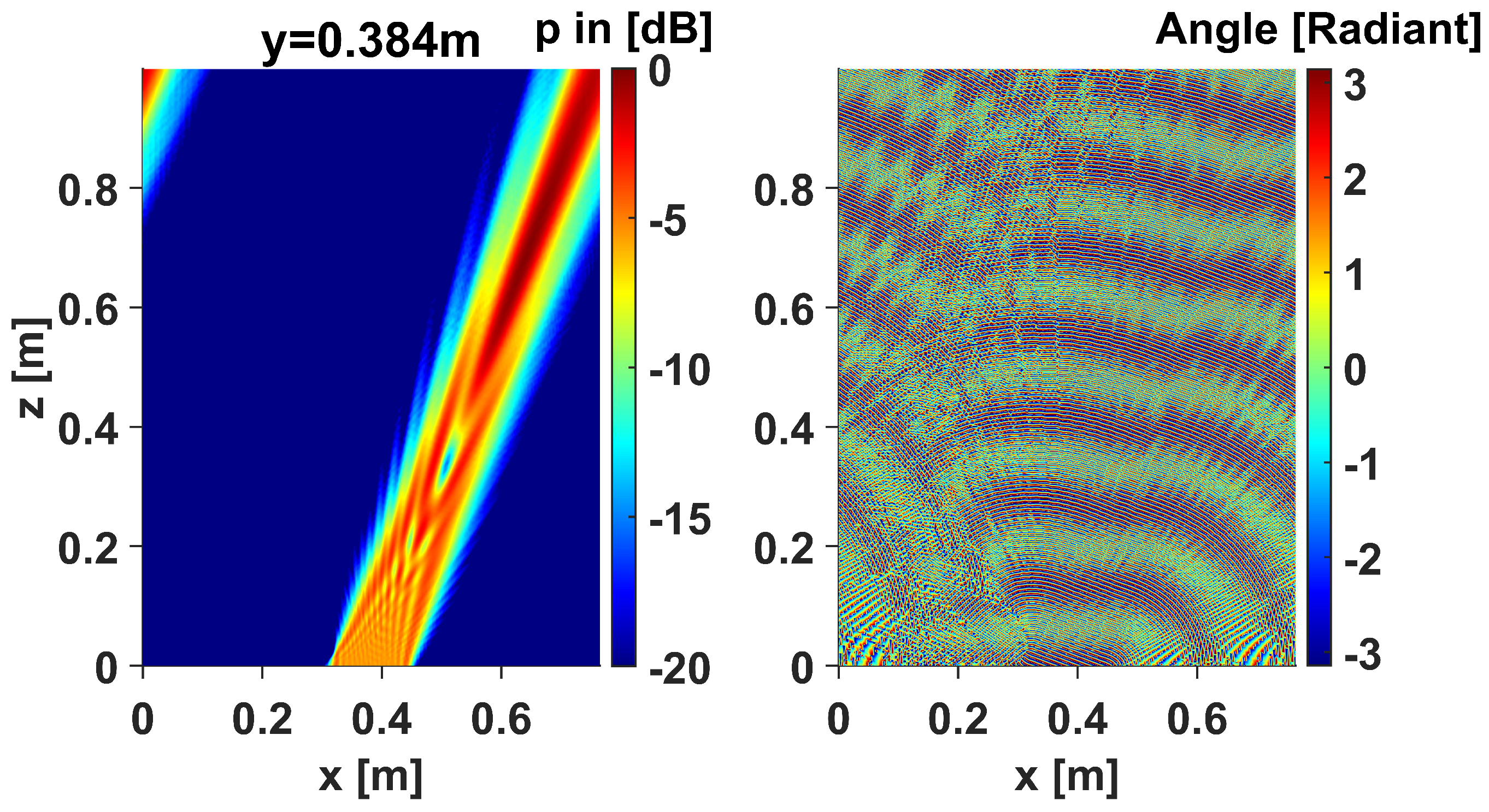
3. Results and Discussion

Various positions in the reconstruction room are discussed in this section. Figure 14 schematically shows these positions. The amplitude of the measured sound field in the measuring plane can be seen in Figure 15 (left). As expected, no flaw could be detected. The sound waves diffracted and interfered so strongly up to the measuring plane that detection of a flaw in this plane was not possible. In Figure 15 (right), the parallel propagation plane (as depicted in Figure 14) can be seen at z = d = 0.22 m. The sound field can be seen to contract again, but the flaw is almost undetectable unless you know it is there. One could also conclude from this image that there are several flaws, or that there is no flaw, but that the sound was transmitted in a slightly different way due to the fibers of the material. Without the knowledge that there is a flaw, it remains a guess about a possible flaw. This plane is also incorrect because the calculation method did not consider solids and the plane went through the particleboard, as depicted in Figure 14. The sound information of this plane, however, could be used to rotate the plane using the procedure in Section 2. For this purpose, it was assumed that this layer (parallel propagation plane) is the z = 0 plane and the plane above the particleboard can be easily defined as in Section 2.3.
This plane did not go through the solid because it was the last plane of air above the particleboard, as depicted in Figure 14 by the angle φ . Figure 16 (left) depicts the determined tilted plane. The flaw is now detectable in position and geometry. The arrow in Figure 16 (left) depicts the position of the flaw and the circle depicts the geometry of the original flaw. For this result, only one plane has to be calculated and rotated. Figure 17 makes the difference between the parallel and the tilted plane more obvious. The yellow area in Figure 16 (left) is slightly smaller than the circle, as well as in Figure 16 (right). This was to be expected, because the piece of paper had a very small curvature toward the center. This curvature was due to the production process, because the paper was punched out with a punch to ensure the exact diameter. Inaccuracies can be seen in Figure 16 (right) because the many planes were calculated and displayed with a grid point distance of 2 mm. In addition, there may have been small inaccuracies during the process of picking out points, because the height of the individual points was determined by the number of planes that were calculated. Here, a distance of the planes of Δ z = 1 mm was chosen. Moreover, the MATLAB function “surf” with the command “shading interp” interpolated the colors over the discrete points. This could also have led to the small inaccuracies in Figure 16 (left and right). In Figure 16 (left), the interpolation of the data in the Fourier domain also had a small influence on the accuracy due to the non-equidistant grid.
This shows that calculations in the tilted plane provide better results than in the parallel propagation plane. Another method to obtain the sound field on the tilted plane is to compute several parallel planes and extract the data of the tilted plane, the results of which are shown in Figure 16 (right). For this purpose, the planes from z = 0.16 m to z = 0.27 m were determined in Δ z = 0.001 m steps according to the size and angle of the plane. It was therefore necessary to calculate 110 planes. In comparison to Figure 16 (left), the calculation of the tilted plane had no noticeable disadvantages. The calculation of a parallel plane currently takes 0.446 s. For 110 planes and the subsequent selecting, this resulted in 49.1 s for the example shown here. However, the calculation of the tilted plane with the proposed method required only 0.721 s. Thus, the calculation of the tilted plane was approximately 98.5% faster than the usual way to evaluate a tilted plane. According to [39], the smallest theoretically detectable flaw has a size of λ / 2 . In [30]. we could already show that, with the spec-radiation method, flaws with a diameter of < λ but > λ /2 can be detected. The λ refers to the medium in which the data are recorded. Similar accuracies could be achieved with the tilted plane. Here, the size and accuracy still depends on the method of rotation in the Fourier space, since, e.g., an interpolation is performed here. This method can also be used for flaws within a particleboard, because these flaws also cause a significant reduction in sound pressure due to the difference in impedance to the board material. This method has thus far been designed to determine the pressure values in the air layer directly above the particleboard. Accordingly, this method can detect any flaw that has a recognizable influence on this layer. With very thick particleboards, where there is a lot of interference inside the material behind the flaw, it is possible that the flaw can no longer be identified from this layer above the board. A computer with the operating system Windows 10 Pro for Workstations and 128 GB RAM and 24 cores of the type Intel(R) Xeon(R) Silver 4116 CPU @ 2.1 GHz was used for the evaluations made here.

4. Conclusions

Herein, we presented the spec-radiation method to determine an additional plane in a sound field parallel to the measuring plane. We extended the spec-radiation method in an innovative way by using the computer holography method. This allowed to rotate the sound field of a plane in the frequency domain for the determination of the sound field of a tilted plane. We presented the method using an academic example of a piston transducer, which showed that this method is suitable for detecting flaws in tilted particleboards. Thus, we were able to overcome the limitations of calculating parallel planes. In particular, the accuracy of flaw detection was significantly improved. We also showed that the procedure is up to 98.5% faster in determining the sound field on the surface of a tilted particleboard than the calculation of many parallel planes and in selecting the corresponding data. We are convinced that these results are a big step toward the real-time analysis of the sound field on the surface of a panel material. Moreover, this is a big advancement toward the use of this sub-wavelength flaw detection method in inline processes.

Author Contributions

Conceptualization, A.S.S. and J.T.; methodology, A.S.S.; software, A.S.S.; validation, A.S.S. and J.T.; formal analysis, A.S.S.; investigation, A.S.S.; resources, A.S.S.; data curation, A.S.S.; writing—original draft preparation, A.S.S.; writing—review and editing, A.S.S. and J.T.; visualization, A.S.S.; supervision, J.T.; project administration, J.T.; funding acquisition, J.T. All authors read and agreed to the published version of the manuscript.

Funding

The publication of this article was funded by the Open Access Fund of Leibniz Universität Hannover.

Acknowledgments

This research was supported by J. Wallaschek.

Conflicts of Interest

The authors declare no conflict of interest.

Abbreviations

The following abbreviations were used in this manuscript:
ToFTime of flight
FFTFast Fourier transformation
iFFTInverse fast Fourier transformation

References

  1. Sokolov, S.Y. On the problem of the propagation of ultrasonic oscillations in various bodies. Elek. Nachr. Tech. 1929, 6, 454–460. [Google Scholar]
  2. Deutsch, V.; Platte, M.; Vogt, M. Ultraschallprüfungen; Springer: Berlin/Heidelberg, Germany, 1997. [Google Scholar] [CrossRef]
  3. Krautkrämer, J.; Krautkrämer, H. Werkstoffprüfung mit Ultraschall; Springer: Berlin/Heidelberg, Germany, 1980. [Google Scholar] [CrossRef]
  4. Lerch, R.; Sessler, G.M.; Wolf, D. Technische Akustik; Springer: Berlin/Heidelberg, Germany, 2009. [Google Scholar] [CrossRef]
  5. Dahmen, S.; Ketata, H.; Ghozlen, M.H.B.; Hosten, B. Elastic constants measurement of anisotropic Olivier wood plates using air-coupled transducers generated Lamb wave and ultrasonic bulk wave. Ultrasonics 2010, 50, 502–507. [Google Scholar] [CrossRef] [PubMed]
  6. Chimenti, D.E. Review of air-coupled ultrasonic materials characterization. Ultrasonics 2014, 54, 1804–1816. [Google Scholar] [CrossRef] [PubMed]
  7. Solodov, I.; Dillenz, A.; Kreutzbruck, M. A new mode of acoustic NDT via resonant air-coupled emission. J. Appl. Phys. 2014, 121, 245101. [Google Scholar] [CrossRef]
  8. Marhenke, T.; Neuenschwander, J.; Furrer, R.; Zolliker, P.; Twiefel, J.; Hasener, J.; Wallaschek, J.; Sanabria, S. Air-coupled ultrasound time reversal (ACU-TR) for subwavelength non-destructive imaging. IEEE Trans. Ultrason. Ferroelectr. Freq. Control 2020, 67, 651–663. [Google Scholar] [CrossRef]
  9. Sanabria Martín, S.J. Air-Coupled Ultrasound Propagation and Novel Non-Destructive Bonding Quality Assessment of Timber Composites; ETH: Zurich, Switzerland, 2012. [Google Scholar] [CrossRef]
  10. Gyekenyesi, A.L.; Harmon, L.M.; Kautz, H.E. The Effect of Experimental Conditions on Acousto-Ultrasonic Reproducibility. Proc. SPIE 2002, 4704, 177–186. [Google Scholar] [CrossRef]
  11. Schafer, M. The Effect of Experimental Conditions on Acousto-Ultrasonic Reproducibility. IEEE Ultrason. Symp. 2000, 771–778. [Google Scholar] [CrossRef]
  12. Jasiuniene, E.; Raisutis, R.; Sliteris, R.; Voleiis, A.; Jakas, M. Ultrasonic NDT of wind turbine blades using contact pulse-echo immersion testing with moving water container. Ultragarsas J. 2008, 63, 28–32. [Google Scholar]
  13. Fang, Y.; Lin, L.; Feng, H.; Lu, Z.; Emms, G.W. Review of the use of air-coupled ultrasonic technologies for nondestructive testing of wood and wood products. Comput. Electron. Agric. 2017, 137, 79–87. [Google Scholar] [CrossRef]
  14. Sanabria, S.; Mueller, C.; Neuenschwander, J.; Niemz, P.; Sennhauser, U. Air-coupled ultrasound as an accurate and reproducible method for bonding assessment of glued timber. Wood Sci. Technol. 2011, 45, 645–659. [Google Scholar] [CrossRef] [Green Version]
  15. Hillger, W.; Bühling, L.; Ilse, D. Review of 30 years ultrasonic systems and developments for the future. In Proceedings of the ECNDT2014, Prague, Czech Republic, 6–10 October 2014. [Google Scholar]
  16. Álvarez Arenas, T.E.G. Acoustic Impedance Matching of Piezoelectric Transducers to the Air. IEEE Trans. Ultrason. Ferroelectr. Freq. Control 2014, 51, 624–633. [Google Scholar] [CrossRef]
  17. Dunky, D.; Niemz, P. Holzwerkstoffe und Leime; Springer: Berlin/Heidelberg, Germany, 2002. [Google Scholar] [CrossRef]
  18. Niemz, P. Bestimmung von Fehlverklebungen mittels Schallaufzeitmessung. Holz Roh Werkst. 1995, 53, 236. [Google Scholar] [CrossRef]
  19. Bucur, V.; Böhnke, I. Factors affecting ultrasonic measurements in solid wood. Ultrasonics 1994, 32, 385–390. [Google Scholar] [CrossRef]
  20. Raichel, D.R. The Science and Applications of Acoustic; Springer Science+Business Media: New York, NY, USA, 2006. [Google Scholar]
  21. Döring, D. Air-Coupled Ultrasound and Guided Acoustic Waves for Application in Non-Destructive Material Testing; OPUS: Stuttgart, Germany, 2011. [Google Scholar] [CrossRef]
  22. Laybed, Y.; Huang, L. Ultrasound time-reversal MUSIC imaging with diffraction and attenuation compensation. IEEE Trans. Ultrason. Ferroelectr. Freq. Control 2012, 59, 2186–2200. [Google Scholar] [CrossRef]
  23. Gabor, D. Holography. Science 1972, 177, 299–313. [Google Scholar] [CrossRef]
  24. Marhenke, T.; Sanabria, S.; Chintada, B.; Furrer, R.; Neuenschwander, J.; Goksel, O. Acoustic field characterization of medical array transducers based on unfocused transmits and single-plane hydrophone measurements. Sensors 2019, 19, 863. [Google Scholar] [CrossRef] [Green Version]
  25. Marhenke, T.; Sanabria, S.; Twiefel, J.; Furrer, R.; Neuenschwander, J.; Wallaschek, J. Three dimensional sound field computation and optimization of the delamination detection based on the re-radiation. In Proceedings of the 12th ECNDT, Gothenburg, Sweden, 11–15 June 2018. [Google Scholar]
  26. Sanabria, S.; Marhenke, T.; Furrer, R.; Neuenschwander, J. Calculation of volumetric sound field of pulsed air-coupled ultrasound transducers based on single-plane measurements. IEEE Trans. Ultrason. Ferroelectr. Freq. Control 2018, 65, 72–84. [Google Scholar] [CrossRef]
  27. Schmelt, A.; Marhenke, T.; Twiefel, J. Identifying objects in a 2D-space utilizing a novel combination of a re-radiation based method and of a difference-image-method. In Proceedings of the ICA 2019, Aachen, Germany, 9–13 September 2019. [Google Scholar]
  28. Schmelt, A.; Marhenke, T.; Hasener, J.; Twiefel, J. Investigation and Enhancement of the Detectability of Flaws with a Coarse Measuring Grid and Air Coupled Ultrasound for NDT of Panel Materials Using the Re-Radiation Method. Appl. Sci. 2020, 10, 1155. [Google Scholar] [CrossRef] [Green Version]
  29. Schmelt, A.; Li, Z.; Marhenke, T.; Twiefel, J. Aussagefähigkeit von Fehlstellenimitaten in der ZfP. In Proceedings of the DAGA2020, Hannover, Germany, 16–19 March 2020; pp. 1133–1136. [Google Scholar]
  30. Schmelt, A.; Twiefel, J. The Spec-Radiation Method as a Fast Alternative to the Re-Radiation Method for the Detection of Flaws in Wooden Particleboards. Appl. Sci. 2020, 10, 6663. [Google Scholar] [CrossRef]
  31. Leseberg, D. Computer-generated three-dimensional image holograms. Appl. Opt. 1992, 31, 223–229. [Google Scholar] [CrossRef]
  32. Nicola, S.D.; Finizio, A.; Pierattini, G.; Ferraro, P.; Alfieri, D. Angular spectrum method with correction of anamorphism for numerical reconstruction of digital holograms on tilted planes. Opt. Express 2005, 13, 9935–9940. [Google Scholar] [CrossRef] [PubMed]
  33. Kostenka, J.; Kozacki, T.; Lizewski, K. Autofocusing method for tilted image plane detection in digital holographic microscopy. Opt. Commun. 2013, 297, 20–26. [Google Scholar] [CrossRef]
  34. Vilardy, J.M.; Jimenez, C.J.; Torres, C.O. Optical Image Encryption System Using Several Tilted Planes. Photonics 2019, 6, 116. [Google Scholar] [CrossRef] [Green Version]
  35. Matsushima, K. Introduction to Computer Holography; Springer Nature Switzerland AG: Cham, Switzerland, 2020. [Google Scholar] [CrossRef]
  36. Goodman, J.W. Introduction to Fourier Optics; W. H. Freeman and Company: New York, NY, USA, 2017. [Google Scholar]
  37. Liu, D.L.; Waag, R.C. Propagation and backpropagation for ultrasonic wavefront design. IEEE Trans. Ultrason. Ferroelectr. Freq. Control 1997, 44, 1–13. [Google Scholar] [CrossRef] [PubMed]
  38. Cramer, O. The variation of the specific heat ratio and the speed of sound in air with temperature, pressure, humidity, and CO2 concentration. J. Acoust. Soc. Am. 1993, 93, 2510–2516. [Google Scholar] [CrossRef]
  39. Wolf, E. Three-dimensional structure determination of semi-transparent objects from holographic data. Opt. Commun. 1969, 1, 153–156. [Google Scholar] [CrossRef]
Figure 1. Schematic representation of the spectrum on the Ewald sphere in the Fourier domain.
Applsci 10 08513 g001
Figure 2. Schematic representation of a tilted particleboard with flaws far away from the propagation plane.
Applsci 10 08513 g002
Figure 3. Amplitude distribution (left) and pressure time signal (right) of the academic piston transducer.
Applsci 10 08513 g003
Figure 4. Amplitude distribution in dB (left) and phase distribution (right) of the academic piston transducer in the Fourier domain at a frequency of 50 kHz.
Applsci 10 08513 g004
Figure 5. Amplitude distribution in dB of the academic piston transducer in the Fourier domain at different wavelengths.
Applsci 10 08513 g005
Figure 6. Schematic representation of the tilted spectrum on the Ewald sphere in the Fourier domain.
Applsci 10 08513 g006
Figure 7. Amplitude distribution in dB (left) and phase distribution (right) of the tilted academic piston transducer in the Fourier domain at a frequency of 50 kHz.
Applsci 10 08513 g007
Figure 8. Amplitude distribution in dB of the academic piston transducer in the Fourier domain at different wavelengths with a tilt.
Applsci 10 08513 g008
Figure 9. Tilted amplitude distribution in dB of the academic piston transducer in the Fourier domain at a frequency of 50 kHz with the considered shift.
Applsci 10 08513 g009
Figure 10. Amplitude distribution in dB (left) and phase distribution (right) of the tilted academic piston transducer in the space domain at a frequency of 50 kHz.
Applsci 10 08513 g010
Figure 11. Amplitude distribution (left) and phase distribution (right) of the tilted academic piston transducer in the space domain at a frequency of 50 kHz propagated with the spec-radiation method in the z direction.
Applsci 10 08513 g011
Figure 12. Experimental setup for the inspection of a tilted particleboard.
Applsci 10 08513 g012
Figure 13. Schematic representation of the placing of the measuring data in the calculation window dx = dy = 4 mm (left) and schematic representation of the placing of the measuring data in the calculation window d x V i r t = d y V i r t = 2 mm (right).
Applsci 10 08513 g013
Figure 14. Schematic reconstruction room.
Applsci 10 08513 g014
Figure 15. Measured amplitude distribution of the refined evaluation grid in the measuring plane in dB related to the maximum of the plane (left). Amplitude distribution of the refined evaluation grid in the parallel propagation plane at z = d = 0.22 m related to the maximum of the plane. The flaw position and size are marked with a cirlce and arrow (right).
Applsci 10 08513 g015
Figure 16. Amplitude distribution of the refined evaluation grid in the tilted plane at z = d = 0.22 m related to the maximum of the plane. The flaw position and size are marked with a circle and arrow and were calculated with the suggested method (left). Determined by the calculation of several parallel planes and the subsequent selection of data (right).
Applsci 10 08513 g016
Figure 17. A 3D image of the amplitude distribution of the parallel propagation plane and the tilted plane above the particleboard.
Applsci 10 08513 g017
Publisher’s Note: MDPI stays neutral with regard to jurisdictional claims in published maps and institutional affiliations.

