Abstract
When damaged by an earthquake, a general structure suffers only primary damage such as in the structure’s collapse, whereas a fluid storage structure can cause secondary damage such as environmental contamination or personal injury due to leakage of its internal fluid. In this study, the flow characteristics of fluid inside a fluid storage structure during an earthquake were analyzed, and an equation to calculate the dynamic hydraulic pressure of the fluid acting on the structure during an earthquake was proposed. The seismic load applied to the fluid storage structure was modified to satisfy the design response spectrum in 300 frequencies so that sufficient earthquake energy was obtained in any natural frequency of the fluid storage structure. In addition, the flow characteristics of the fluid inside the fluid storage structure were examined according to the shape change of the seismic wave and the ratio of the height of the fluid to the width of the fluid storage structure. A resulting equation for calculating the hydraulic pressure reflecting the fluctuation characteristics of the fluid was derived, and structural analysis was performed based on this equation and equations proposed by prior research to compare the member force and the hydraulic pressure in a dangerous section. As a result, it was confirmed that the equation proposed in this study showed similar values to previously proposed equations and could obtain fairly reliable results. Therefore, based on the proposed equation in this study, it is possible to calculate hydraulic pressure by reflecting the free-water surface fluctuation characteristics of fluid inside a fluid storage structure during an earthquake.
1. Introduction
Around the world, the magnitude and the frequency of seismic activity are increasing, and so too are the effects on property and human lives. The 1999 Taiwan earthquake resulted in over 2000 casualties and some 10 billion dollars of damage to property, and the earthquake of magnitude 7 in Haiti in 2010 caused tens of thousands of casualties, with the collapse of social infrastructure resulting in massive economic losses. The earthquake and tsunami that occurred in Japan in 2011 resulted in more than 10,000 lost lives as well as the explosion at and subsequent leakage of hazardous radioactive isotopes from the Daiichi nuclear power plant. When a structure is damaged due to an earthquake, general structures incur only primary damage such as collapse, but fluid storage structures can cause secondary damage such as environmental pollution or personal injury from the escape of internal fluid. To prevent such disasters, it is important for a fluid storage structure to accurately contain the flow characteristics of the fluid inside the structure and for the fluid dynamic pressure acting on the structure to be accurately calculated [1].
To calculate the hydraulic pressure of a fluid, Westergaard [2] developed a theoretical equation for the hydraulic pressure acting on a structure when an earthquake occurs in a vertical dam, ands proposed an approximate solution. Based on the approximate solution, some of the water stored in the reservoir is loaded on to the dam body as an additional mass, and the concept of generating a load equal to the hydraulic pressure on the dam body by the seismic force applied to the added mass during an earthquake was additionally proposed. Housner [3,4] proposed a mechanics-based method of modeling the dynamic effects of fluid inside a fluid storage structure by seismic loads as convective mass and impact mass, assuming that the structure wall is a rigid body, and Chopra [5,6,7,8] found a theoretical solution to the hydraulic pressure generated during earthquakes in a vertical dam in a lake composed of compressible fluid. Fischer [9] conducted a study on a brief seismic response analysis method for flexible tanks based on the boundary solution induced by the analysis, and Haroun [10] proposed a method of modeling a structure as an axisymmetric finite element (FE) for the detailed seismic response analysis of a cylindrical fluid storage tank and analyzed the fluid region using a fluid-added mass matrix based on the boundary analysis method. Due to the recent development of numerical analysis techniques, various analysis techniques that can directly model fluid inside a fluid storage structure have been proposed. Through such analysis methods, studies have begun to analyze flow characteristics inside a fluid storage structure under seismic loads and to compare and analyze similarities with experiments. However, most of these studies only estimate the fluctuation characteristics of internal fluid by repeatedly loading the same load or using a sine wave, so it is difficult to estimate the fluid flow characteristics and hydraulic pressure generated by a real earthquake [11]. Several other dynamic hydraulic pressure studies have analyzed the flow characteristics of fluid inside a fluid storage structure when a real earthquake occurs as well as the hydraulic pressure acting on the wall of a fluid storage structure [12,13]. However, each real earthquake has its own characteristics, so any analyzed fluid flow characteristics and hydraulic pressure cannot necessarily be considered representative results for all earthquakes.
Westergaard and Housner proposed well-known equations for calculating hydraulic pressure that have been applied in actual designs. However, Westergaard’s equation is suited to dams, not to other types of structures, because Westergaard’s equation does not take into account the width of a structure (or the width of the fluid), only the height. Therefore, even if a structure’s width changes, the hydraulic pressure of the fluid always remains constant. Housner’s equation, on the other hand, is suited to a broader range of structures, but even so, many storage tanks designed based on Housner’s equation were damaged by the Alaska earthquake of 1964 [14]. This study proposes an equation for calculating the hydraulic pressure of fluid that can be used in the design of a fluid storage structure when a seismic load is applied. Various design codes provide standards for seismic loads; the most detailed standards are presented by the U.S. Nuclear Regulatory Commission Regulatory Guides (U.S. NRC RGs). For example, U.S. NRC RG 1.60 presents design response spectra for various damping ratios (0.5%, 2%, 5%, 7%, 10%), and U.S. NRC RG 1.122 presents detailed requirements for seismic loads to be applied to a design. The detailed requirements for seismic loads presented in U.S. NRC RG 1.122 are as follows:
- The response spectrum obtained from the seismic load should cover the design response spectrum in the damping ratio used in the seismic response analysis;
- When calculating spectral values (e.g., spectral acceleration) from artificial seismic waves, the frequency interval for calculating spectral values should be sufficiently small.
The U.S. NRC RG 1.122 presents the criteria for frequency intervals for calculating spectral values from multiple damping ratios, and U.S. NRC RG 3.7.1 provides criteria for frequency intervals for calculating spectral values from single damping ratios. This study was conducted by generating a seismic load that satisfies the various requirements proposed by the U.S. NRC RGs. To do this, the seismic load was generated using the software, SIMQKE [15]. However, the seismic load generated by SIMQKE cannot satisfy the U.S. NRC RGs. Lilhanand [16,17] conducted a study on a technique that can cover the response spectrum by modifying the seismic load using the impact response function. The technique proposed by Lilhanand is sufficient to modify the seismic load created by SIMQKE to satisfy the U.S. NRC RGs. The seismic load used in this study was modified using the technique proposed by Lilhanand to satisfy the U.S. NRC RGs.
There are many factors that influence the behavior of the fluid inside a fluid storage structure when a seismic load is applied. The most accurate results can be obtained when research is conducted considering all factors, but in reality that is almost impossible. Therefore, it is very important to select the factor(s) that most sensitively affect(s) the fluctuation characteristics of the fluid. In this study, the seismic load shape and the ratio of the width of the structure and the height of the fluid were selected as important factors among a number of factors. The ratio of the width of the structure to the height of the fluid is closely related to the shape of the fluid. If fluids with different heights are stored in structures having the same width, the total volume and mass of the fluid are different, and this most greatly influences the fluid fluctuation characteristics when a seismic load is applied. The seismic load shape was selected as an important factor because the effect of the shape of the seismic load on the fluctuation characteristics of the fluid cannot be clearly known. This is because even if the seismic load satisfies a design code, it is difficult to derive consistent results if the fluid shape fluctuates according to changes in shape. The peak acceleration is also considered to be an important factor influencing the fluctuation characteristics of the fluid. However, in general, design codes clearly state the peak acceleration (e.g., Korean Highway Bridge Design Code: 0.154 g, U.S. NRC RGs: 0.3 g). The peak acceleration of 0.3 g was applied based on the U.S. NRC RGs because it can yield the most conservative results.
The experiment was performed by varying the ratio of the width of the fluid storage structure to the height of the fluid. The experiment result was used as verification data of Abaqus, the commercially available FE analysis software. If the verification result of the program secured sufficient validity to replace the experiment, the program could be used to analyze various variables. The most important consideration in the FE model applied in this study was fluid. Various elements have been proposed to apply fluid to an FE model, and smoothed-particle hydrodynamics (SPH) elements have recently been used in large deformation problems such as fluid [18,19,20,21]. Therefore, the fluid was modeled using SPH elements as its reliability has been verified in previous work.
2. Shaking Table Test with Scaled Model and Verification Analysis
Applying seismic loads to a fluid storage structure is practically limited when trying to experimentally identify all factors that affect the dynamic characteristics of a free-water surface in a fluid storage structure. Therefore, in order to replace the experimental limitations analytically, a scaled model test was performed, and an analysis was conducted with the smoothed-particle hydrodynamics (SPH) method, a fluid–structure interaction analysis technique, and the results of the experiment and the analysis were compared and analyzed.
2.1. Shaking Table Test with Scaled Model
In order to verify the similarity between the fluid–structure interaction analysis applying the SPH method and the scaled model test, an acrylic tank was constructed with the shape and specifications shown in Figure 1. The dimensions of the tank were 500 (width), 400 (height), and 10 (thickness), and the heights of the fluid inside the tank were 125 and 200 mm, which were 25% and 40% of the width of the tank, respectively. The shaking table used in the test loaded the seismic load on to the scaled model through displacement control. The shaking table experiment was performed using the time-displacement of the real earthquake shown in Figure 2a, and the time-acceleration acting on the scaled model was measured using an accelerometer attached to the bottom of the shaking table. The measured time-acceleration curve is shown in Figure 2b.
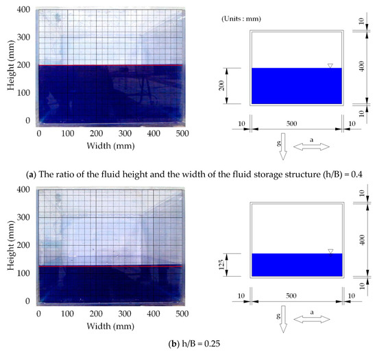
Figure 1.
Scaled model and specification.
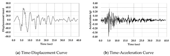
Figure 2.
Input time-history curve and measured time-acceleration curve.
When the same seismic load was applied, as the ratio of the width of the fluid storage structure and the height of the internal fluid changes, the maximum sloshing height, free-water surface shape, and time-sloshing height of the fluid were experimentally confirmed, and the results are shown in Figure 3 and Table 1. When the ratio of the fluid height and the width of the fluid storage structure (h/B) was 0.4, the time for the maximum sloshing height to occur was 6.000 s, and the measured maximum and minimum sloshing heights of the fluid were 308.0 and 168.0 mm. Considering the initial fluid height of 200 mm, the maximum fluid height rose to 154% of the initial fluid height, and the minimum height fell to 84% of the initial fluid height. In addition, when h/B was 0.25, the time for the maximum sloshing height to occur was 6.020 s, and the maximum and the minimum sloshing heights of the fluid generated at this time were measured as 247.0 and 95.0 mm. Considering the initial fluid height of 125 mm, the maximum sway height of the fluid rose to 198% and the minimum sway height fell to 76%. From these experimental results, it can be seen that as h/B increases, the maximum and the minimum sloshing heights of the fluid tend to decrease.
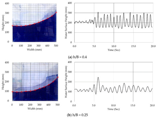
Figure 3.
Shaking table test result for the scaled model.

Table 1.
Results summary of the scaled model shaking table test.
2.2. Verification Analysis
For comparison between the scaled model test and the analysis, a seismic analysis was performed with the structural analysis model shown in Figure 4 using Abaqus. In the analysis, the acrylic tank was modeled by applying an 8-node solid element (C3D8R), and the fluid was modeled by applying a continuum particle element (PC3D). The continuum particle element is a one-node element, having the solid characteristic of a three-DOF system and developed for the analysis of phenomena that cause extreme deformation, such as fluid flow or structure collapse. The material properties of the acrylic tank were determined based on the research of Vesenjak et al. [22], and the unit weight, elastic modulus, and Poisson’s ratio of the fluid and acrylic tank are as shown in Table 2. A linear Us-Up Hugoniot was used for the linear equation of state to determine the fluid flow characteristics (Abaqus/Analysis User’s Guide Volume III, Materials 2014), and it can be expressed as Equation (1). The parameters applied to the linear equation are shown in Table 2.
where and define the linear relationship between the linear shock velocity, and is the particle velocity.
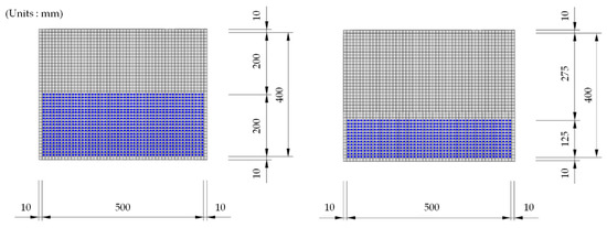
Figure 4.
Finite element model for validation analysis.
Table 2.
Summary of elements and materials applied to validation analysis.
The maximum and minimum sloshing height and occurrence time of the fluid water surface obtained from the experiment and analysis are compared and shown in Figure 5 and Table 3. When the ratio of the fluid height and the width of the fluid storage structure (h/B) was 0.40, the time for the maximum sloshing height to occur was 6.000 s in the experiment and 6.020 s wan the analysis. It was confirmed that the maximum sloshing height by the experiment and analysis occurred at almost the same time. When h/B was 0.25, the time for the maximum sloshing height to occur was 6.020 s in the experiment and analysis. When h/B was 0.40, the maximum sloshing height of the water surface occurred at 308.0 mm in the experiment and 317.0 mm in the analysis, confirming that the error between the experiment and the analysis was 2.839%. In addition, the minimum sloshing height of the water surface occurred at 168.0 mm in the experiment and 160.0 mm in the analysis, confirming that the error between the experiment and the analysis was 5.0%. When h/B was 0.25, the maximum sloshing height of the water surface was 247.0 mm in the experiment and 249.0 mm in the analysis, confirming that the error between the experiment and the analysis was 0.810%. In addition, the minimum sloshing height of the water surface was 95.0 mm in the experiment and 97.0 mm in the analysis, confirming that the error between the experiment and analysis was 5.0%. Based on the above results, it was confirmed that the fluid–structure interaction analysis by the SPH method predicts the dynamic properties of the fluid surface very accurately.
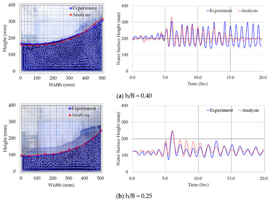
Figure 5.
Comparison of sloshing height from experiment and analysis.
Table 3.
Comparison of sloshing height between experiment and analysis.
3. Results
When a seismic load of different shapes with the same peak acceleration satisfying the design code act on a fluid storage structure, the flow characteristics of the fluid surface can be analyzed. In addition, when the same seismic load acts on a fluid storage structure, the flow characteristics of the fluid surface were identified as the ratio of the width of the fluid storage structure, and the height of the fluid changed. Based on this result, this study proposes an equation that can estimate the shape of a fluid surface as the ratio of the width of a fluid storage structure and the height of fluid surface changes. In addition, the validity of the proposed equation in this study was verified by comparing the proposed equation with equations proposed by previous research.
3.1. Dynamic Behavior of Fluid Surface According to the Seismic Load Shape
In order to understand the dynamic characteristics of a fluid surface according to the shape of the seismic wave, SIMQKE was used to generate five seismic waves with arbitrary shapes. Since the seismic load randomly created by SIMQKE could not satisfy the design code, the seismic load was modified through a seismic load correction method, and the modified seismic load was compared with the design response spectrum proposed in U.S. NRC RG 1.60. Figure 6 shows the seismic load applied to the fluid–structure interaction analysis (left side) and the comparison of the response spectrum calculated by the modified seismic load and the design response spectrum (right side).

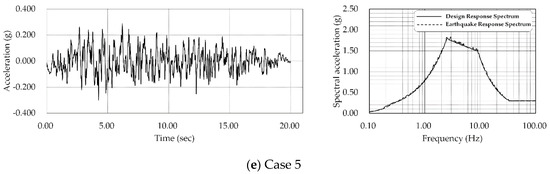
Figure 6.
Modified earthquake and comparison of design and earthquake response spectrum.
The element and material characteristics of the numerical analysis model applied to the fluid–structure interaction were the same as the model applied to the verification analysis. The shape, specification, and height of the fluid are as shown in Figure 7.
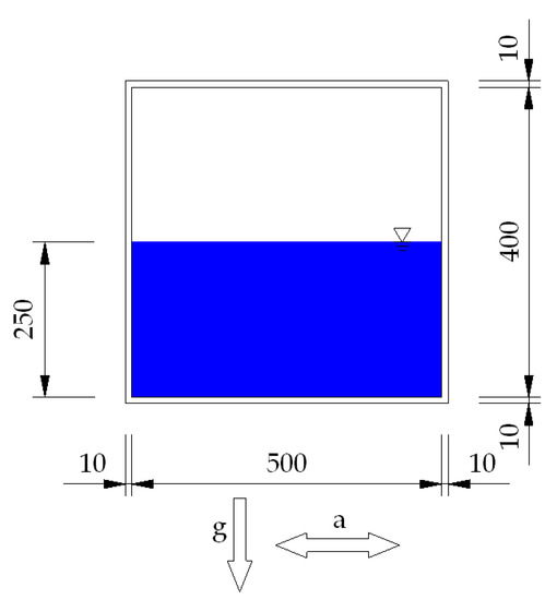
Figure 7.
Analytical model for evaluating the effects of earthquake of different shapes.
Table 4 shows the time when the maximum sloshing height occurred on the fluid surface and the maximum sloshing height and the minimum sloshing height of the fluid surface, and Figure 8 shows the shape at the time when the maximum sloshing height occurred on the fluid surface. The maximum sloshing height of the fluid surface was measured as 363, 363, 369, 368, and 369 mm, and the minimum height was measured as 180, 183, 183, 184, and 182 mm, depending on the seismic load. The seismic loads that generated the value of 369 mm, which is the largest of the maximum sloshing heights of the fluid surface generated by the five artificial seismic loads, were Case 3 and Case 5, and the seismic loads that generated the smallest sloshing height of 363 mm were Case 1 and Case 2. When comparing the maximum sloshing height generated by the five earthquake loads, it was found that the difference between the largest and the smallest values of the maximum sloshing height was about 1.6%. When comparing the minimum sloshing height generated by the five seismic loads, the difference between the largest and the smallest values of the minimum sloshing height was about 2.2%, confirming that the shape of seismic loads was not affected the maximum and minimum sloshing height. Comparing the shape of the fluid surface generated by different shape seismic loads showed an error of up to 9.244% at all points, meaning that the seismic load shape was not affected by the shape of the fluid surface, or maximum and minimum sloshing height.
Table 4.
Summary of slushing heights generated by earthquakes of different shapes.
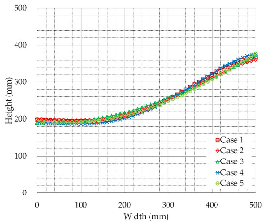
Figure 8.
Comparison of fluid surface shape by earthquakes of different shapes.
The seismic load applied in this study followed the U.S. NRC RGs. Seismic loads generated according to the U.S. NRC RGs had a value similar to the design response spectrum in all calculated frequencies. In other words, even if the shape of the seismic load applied in this study was different, converting it into a response spectrum meant that it had similar spectral acceleration values in all calculated frequencies. This means that in the frequency corresponding to the natural frequency of the fluid inside the fluid storage structure, if the seismic load spectral acceleration of different shapes was the same, the fluid fluctuation shape occurred similarly.
3.2. Dynamic Characteristics of Fluid Surface According to the Ratio of Fluid Height and Structure Width
The h/B was set at 200, 250, 300, 350, and 400 mm (h/B: 0.4, 0.5, 0.6, 0.7, and 0.8) in order to estimate the dynamic characteristics of the fluid surface according to the ratio of the width of the fluid storage structure to the initial fluid height. The specifics of the structure applied to the analysis are shown in Figure 9, and the analysis was performed by applying the seismic load shown in Figure 6a.
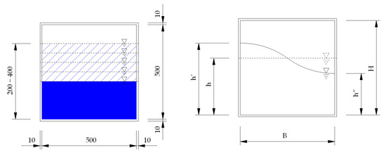
Figure 9.
Analytical model for evaluating the influence of fluid height and structure width.
Figure 10 shows the shape of the fluid surface at 7.300, 6.790, 8.050, 12.930, and 12.910 s, which are the times when the maximum sloshing height of the fluid surface occurs. As shown in Table 5, as the ratio h/B of the fluid height and the width of the structure increased from 0.4 to 0.8 by 0.1, the maximum sloshing height was measured as 287, 338, 398, 471, and 500 mm, and the minimum sloshing height was measured as 156, 206, 240, 287, and 338 mm. However, when h/B was 0.8, the maximum sloshing height could not be accurately measured because the fluid surface was in contact with the upper slab.
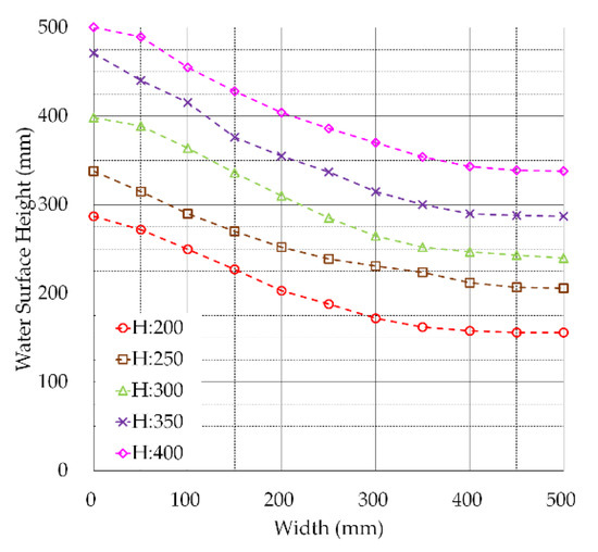
Figure 10.
Comparison of fluid surface shape from ratio of initial fluid height to structure width.
Table 5.
Maximum and minimum sloshing height according to h/B.
Table 6 shows the fluid height to structure width ratio (h/B) and the initial fluid height to maximum sloshing height ratio (h’/h) based on the results shown in Table 5 and Figure 10. It can be seen that as the h/B decreases, that is, as the ratio of the fluid height to width of the fluid storage structure decreases, the maximum sloshing height of the fluid increases.
Table 6.
Ratio of the initial fluid height to the maximum sloshing height according to h/B.
Through regression analysis of the fluid height to structure width ratio (h/B) and the initial fluid height to maximum sloshing height ratio (h′/h), it was confirmed that there is a relationship between Equation (2) and that the correlation coefficient R2 was 0.811.
where is the width of the fluid storage structure, is the initial fluid height, and is maximum sloshing height. Table 7 shows the relationship between h/B and the ratio of the initial fluid height and the minimum sloshing height (h″/h). It can be seen that the smaller the h/B, that is, the lower the ratio of the fluid height and the width of the fluid storage structure, the lower the minimum sloshing height of the fluid. Through regression analysis of the fluid height to structure width ratio (h/B) and the initial fluid height to maximum sloshing height ratio (h″/h), it was confirmed that there was a relationship between Equation (3) and the correlation coefficient R2 of 0.848.
Table 7.
Ratio of the initial fluid height to the minimum sloshing height according to h/B.
In this study, the shape of the fluid surface during a seismic load was assumed to be a straight line (the most simplified form) and can be represented as Equation (4).
where α is the amplitude coefficient due to the fluctuation of the fluid surface and β is the coefficient related to the initial height of the fluid, shown as Equation (5) by the shape function of the fluid surface.
where is the width of the fluid storage structure, and is the initial fluid height. Table 8 shows the comparison of the maximum sloshing height and minimum sloshing height of the fluid surface by numerical analysis and the proposed equation. The maximum sloshing height of the fluid shown by the numerical analysis and the proposed equation showed a difference of 1.186~3.040%, and the minimum sloshing height showed a difference of 0.734~2.791%. Therefore, the sloshing height of the fluid surface by the proposed equation and numerical analysis were similar.
Table 8.
Maximum and minimum sloshing height predicted by the proposed equation according to h/B.
3.3. Proposal and Verification of Dynamic Hydraulic Pressure Calculation Method
The method for calculating the dynamic hydraulic pressure proposed in this study is based on the method proposed by Housner. Therefore, as shown in Figure 11, the dynamic hydraulic pressure of the fluid was divided into convective components and impulsive components, and the dynamic hydraulic pressure of the convective and impulsive components could be calculated by Equations (6) and (7).
where is the width of the fluid storage structure, is the initial fluid height, is the minimum of sloshing height, and is the weight density. In order to verify the proposed equation in this study, methods proposed by existing work and that of this study were used to apply dynamic hydraulic pressure to an arbitrary structure to compare the member forces of a dangerous section. The structure size applied in the analysis was 10.0 (width) and 5.0 m (height), and it was assumed that 3.0 m of fluid was contained in the structure with the thickness of the wall 0.3, upper slab 0.3, and floor slab 0.5 m. For time-history analysis, a numerical analysis model was generated using MIDAS, the commercially available FE analysis program, and the seismic load shown in Figure 6b was applied.
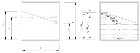
Figure 11.
Dynamic pressure distribution of proposed model.
After performing the time-history analysis of the FE model considering the fluid, the bending moment, shear force, and reaction force generated in the dangerous section of the wall were compared, as displayed in Table 9. Comparing the total hydraulic pressure acting on the structure, the Housner model was 176.5 kN, which was about 80% of the existing and proposed models. The maximum bending moment and the maximum shear force in the dangerous section were estimated to be only about 50% of the Housner model compared with other existing models and the proposed models. Therefore, it was confirmed that the Housner model was underestimated compared with existing and proposed models. However, in the proposed model in which the dynamic hydraulic pressure of fluid was applied to the wall in the same form as the Housner model, the total hydraulic pressure acting on the structure was estimated to be 220.9 kN, indicating an error of 1–7% from the existing model. Therefore, it was confirmed that the hydraulic pressure calculated by the proposed model had similar values to the existing models, except for Housner’s model. When comparing the maximum bending moment and the maximum shear force in the dangerous section, the values calculated by the proposed model had similar values to all of the existing models except for Housner’s. From the results, it can be concluded that the structural analysis of a fluid storage structure by the proposed model can sufficiently secure the safety of a structure while approximately simulating the dynamic behavior of the fluid.
Table 9.
Comparison of member force from each model.
4. Conclusions and Future Work
In this study, an equation for calculating the hydraulic pressure generated by the fluid inside a fluid storage structure when a seismic load is applied was proposed. A critical factor in designing for earthquake resistance was the seismic load acting on a structure, precisely because of the uncertainty of the seismic load. Various design codes provide standards for seismic loads, but the U.S. NRC RGs provide the most detailed seismic load standards; therefore, in this study, seismic loads were generated to satisfy the U.S. NRC RGs. In order to satisfy the U.S. NRC RGs, a seismic load generated using SIMQKE was modified. The modification of the seismic load was performed by referring to Lilhanand’s study, and as a result, it was confirmed that the standards proposed by the U.S. NRC RGs were satisfied. Therefore, the results of this study are considered to reflect structural characteristics more accurately than study results using real earthquakes. This means that the results of this study are sufficiently conservative and can be prevented from leading to excessive results.
An experiment was performed on a fluid–structure interaction, and the result was used to verify the analysis program (Abaqus). The smoothed-particle hydrodynamics (SPH) method has been widely used to solve the problem of large deformation involving a fluid, and SPH was chosen for this study’s analysis method. Although reliability has been verified in prior studies, reliability was verified once again through the comparison of experiment and analysis. As a result, it was confirmed that the maximum sloshing height, minimum sloshing height, fluid surface shape, and time-sloshing height curve predicted by the SPH method used in this study were similar to the experimental results. Therefore, it is considered that sufficient reliability can be secured even by performing various parameter analyses using the SPH method.
Analysis of various variables was performed to calculate the hydraulic pressure of the fluid inside a fluid storage structure. First, the effect of the seismic load shape on the fluid fluctuation characteristics was analyzed. Seismic loads of five different shapes were applied to the same structure, and the fluid fluctuations were compared. As a result, even if the shape of the seismic load changed, the fluctuation characteristics of the fluid inside the fluid storage structure were unchanged. This is considered to be related to the seismic load characteristics used in this study. The shape of the seismic load used in this study was different, but the values of the spectral acceleration were similar when converted to a response spectrum. This means that even if the shape of the seismic load was different, if the structure had a similar spectral acceleration value in the natural frequency of the structure, the fluctuation characteristics of the fluid occurred similarly. Second, the effect of the structure width and fluid height on the fluid fluctuation shape was analyzed. It was confirmed that as the ratio of the width of the structure and the height of the fluid increased, the maximum sloshing height of the fluid decreased.
Various variables were analyzed, and based on the results, an equation for the fluid dynamic hydraulic pressure was proposed when a seismic load was applied. The equation proposed in this study can accurately derive the maximum and minimum sloshing height of the fluid. This means that the action point of the impulsive mass and the convective mass of the fluid can be accurately calculated. A more accurate calculation is consequently possible compared with the previously suggested formula. This is considered a very important part in the design of the structure. However, in this study, only the seismic load shape and the change in ratio of the initial fluid height to the structure width were used as variables when a seismic load with a peak acceleration of 0.3 g was applied to a rectangular structure. Therefore, with additional studies on the shape of the fluid storage structure, the change in the peak acceleration, and the stiffness of the structure, local goodness-of-fit estimates from a cross-validation analysis or with a training/test could be conducted.
Author Contributions
Conceptualization, G.P.; methodology, G.P.; software, G.P.; validation, H.Y. and K.-N.H.; formal analysis, G.P.; investigation, G.P.; resources, G.P.; data curation, G.P.; writing—original draft preparation, G.P.; writing—review and editing, H.Y. and K.-N.H.; visualization, G.P.; supervision, H.Y.; project administration, K.-N.H.; funding acquisition, G.P. All authors have read and agreed to the published version of the manuscript.
Funding
This work is supported by the Korea Agency for Infrastructure Technology Advancement (KAIA) grant funded by the Ministry of Land, Infrastructure and Transport (Grant 20CTAP-C152100-02).
Conflicts of Interest
The authors declare no conflict of interest.
References
- Son, I.-M.; Kim, J.-M.; Choi, H.-S.; Baek, E.-R. Post-correlation analysis for shake table test of square liquid storage tank. J. Korea Inst. Struct. Maint. Insp. 2017, 21, 23–29. [Google Scholar]
- Westergaard, H.M. Water pressures on dams during earthquakes. Trans. ASCE 1933, 95, 418–433. [Google Scholar]
- Housner, G.W. Dynamic Analysis of Fluids in Containers Subjected to Acceleration. In Nuclear Reactors and Earthquakes; Report No. TID; U.S. Atomic Energy Commission: Washington, DC, USA, 1963; p. 7024. [Google Scholar]
- Lebbi, I.; Moslemian, J. Recent Revisions of SRP 3.7 and 3.8. In Proceedings of the Pressure Vessels and Piping Conference, American Society of Mechanical Engineers 2015, Boston Park Plaza, Boston, MA, USA, 19–23 July 2015; Volume 57034, p. V008T08A033. [Google Scholar]
- Chopra, A.K. Hydrodynamic pressures on dams during earthquakes. J. Eng. Mech. Div. 1967, 93, 205–224. [Google Scholar]
- Chopra, A.K. Reservoir-dam interaction during earthquakes. Bull. Seismol. Soc. Am. 1967, 57, 675–687. [Google Scholar]
- Chopra, A.K. Earthquake behavior of reservoir-dam systems. J. Eng. Mech. Div. 1968, 94, 1475–1500. [Google Scholar]
- Chopra, A.K. Earthquake Response of Concrete Gravity Dams. J. Eng. Mech. Div. 1970, 96, 443–454. [Google Scholar]
- Fischer, D. Dynamic fluid effects in liquid-filled flexible cylindrical tanks. Earthq. Eng. Struct. Dyn. 1979, 7, 587–601. [Google Scholar] [CrossRef]
- Haroun, M.A. Dynamic Analyses of Liquid Storage Tanks. Report No. EERL 80-4, Earthquake. Available online: https://authors.library.caltech.edu/26356/ (accessed on 17 November 2020).
- Brizzolara, S.; Savio, L.; Viviani, M.; Chen, Y.; Temarel, P.; Couty, N.; Hoflack, S.; Diebold, L.; Moirod, N.; Iglesias, A.S. Comparison of experimental and numerical sloshing loads in partially filled tanks. Ships Offshore Struct. 2011, 6, 15–43. [Google Scholar] [CrossRef]
- Shimada, S.; Noda, S.; Yoshida, T. Nonlinear sloshing analysis of liquid storage tanks subjected to relatively long-period motions. In Proceedings of the Ninth World Conference on Earthquake Engineering, Tokyo-Kyoto, Japan, 2–9 August 1988; Volume VI, pp. 613–618. [Google Scholar]
- Koh, H.M.; Kim, J.K.; Park, J.-H. Fluid–structure interaction analysis of 3-D rectangular tanks by a variationally coupled BEM–FEM and comparison with test results. Earthq. Eng. Struct. Dyn. 1998, 27, 109–124. [Google Scholar] [CrossRef]
- Lee, C.G.; Yun, C.B. Seismic Analysis of Liquid Storage Tanks Considering Shell Flexibility. J. Korean Soc. Civ. Eng. 1987, 7, 21–29. [Google Scholar]
- Gasparini, D.; Vanmarcke, E.H. SIMQKE: A Program for Artificial Motion Generation; Department of Civil Engineering, Massachusetts Institute of Technology: Cambridge, MA, USA, 1976. [Google Scholar]
- Lilhanand, K.; Tseng, W.S. Generation of synthetic time histories compatible with multiple-damping design response spectra. In Proceedings of the Transactions of the 9th International Conference on Structural Mechanics in Reactor Technology, Lausanne, Switzerland, 17–21 August 1987; Volume K1. [Google Scholar]
- Lilhanand, K.; Tseng, W.S. Development and application of realistic earthquake time histories compatible with multiple-damping design spectra. In Proceedings of the 9th World Conference on Earthquake Engineering, Tokyo-Kyoto, Japan, 2–9 August 1988; Volume 2, pp. 819–824. [Google Scholar]
- Aly, A.M.; Raizah, Z.A.S. Incompressible smoothed particle hydrodynamics simulation of natural convection in a nanofluid-filled complex wavy porous cavity with inner solid particles. Phys. A Stat. Mech. Appl. 2020, 537, 122623. [Google Scholar] [CrossRef]
- Koschier, D.; Bender, J.; Solenthaler, B.; Teschner, M. Smoothed particle hydrodynamics techniques for the physics based simulation of fluids and solids. arXiv 2020, arXiv:2009.06944. [Google Scholar]
- Garoosi, F.; Shakibaeinia, A. Numerical simulation of free-surface flow and convection heat transfer using a modified Weakly Compressible Smoothed Particle Hydrodynamics (WCSPH) method. Int. J. Mech. Sci. 2020, 188, 105940. [Google Scholar] [CrossRef]
- Huntley, S.; Rendall, T.; Longana, M.; Pozegic, T.; Potter, K.; Hamerton, I. Validation of a smoothed particle hydrodynamics model for a highly aligned discontinuous fibre composites manufacturing process. Compos. Sci. Technol. 2020, 196, 108152. [Google Scholar] [CrossRef]
- Vesenjak, M.; Mullerschon, H.; Hummel, A.; Ren, Z. Simulation of Fuel Sloshing-Comparative Study; LS-DYNA Anwend: Bamberg, Germany, 13–14 October 2004. [Google Scholar]
Publisher’s Note: MDPI stays neutral with regard to jurisdictional claims in published maps and institutional affiliations. |
© 2020 by the authors. Licensee MDPI, Basel, Switzerland. This article is an open access article distributed under the terms and conditions of the Creative Commons Attribution (CC BY) license (http://creativecommons.org/licenses/by/4.0/).