Article

Short-Term Forecasting of Photovoltaic Solar Power Production Using Variational Auto-Encoder Driven Deep Learning Approach

1
Computer Science Department Signal, Image and Speech Laboratory (SIMPA) Laboratory, University of Science and Technology of Oran-Mohamed Boudiaf (USTO-MB), El Mnaouar, BP 1505, Bir El Djir 31000, Algeria
2
Computer, Electrical and Mathematical Sciences and Engineering (CEMSE) Division, King Abdullah University of Science and Technology (KAUST), Thuwal 23955-6900, Saudi Arabia
3
Department of Electrical Engineering, University of Sharjah, Sharjah 27272, UAE
*
Author to whom correspondence should be addressed.
These authors contributed equally to this work.
Appl. Sci. 2020, 10(23), 8400; https://doi.org/10.3390/app10238400
Submission received: 7 October 2020 / Revised: 17 November 2020 / Accepted: 19 November 2020 / Published: 25 November 2020

Abstract

:
The accurate modeling and forecasting of the power output of photovoltaic (PV) systems are critical to efficiently managing their integration in smart grids, delivery, and storage. This paper intends to provide efficient short-term forecasting of solar power production using Variational AutoEncoder (VAE) model. Adopting the VAE-driven deep learning model is expected to improve forecasting accuracy because of its suitable performance in time-series modeling and flexible nonlinear approximation. Both single- and multi-step-ahead forecasts are investigated in this work. Data from two grid-connected plants (a 243 kW parking lot canopy array in the US and a 9 MW PV system in Algeria) are employed to show the investigated deep learning models’ performance. Specifically, the forecasting outputs of the proposed VAE-based forecasting method have been compared with seven deep learning methods, namely recurrent neural network, Long short-term memory (LSTM), Bidirectional LSTM, Convolutional LSTM network, Gated recurrent units, stacked autoencoder, and restricted Boltzmann machine, and two commonly used machine learning methods, namely logistic regression and support vector regression. The results of this investigation demonstrate the satisfying performance of deep learning techniques to forecast solar power and point out that the VAE consistently performed better than the other methods. Also, results confirmed the superior performance of deep learning models compared to the two considered baseline machine learning models.

1. Introduction

The accurate modeling and forecasting of solar power output in photovoltaic (PV) systems are certainly essential to improve their management and enable their integration in smart grids [1,2]. Namely, the output power of a PV system is highly correlated with the solar irradiation and the weather conditions that explain the intermittent nature of PV system power generation. Particularly, the characteristic of fluctuation and intermittent of the temperature and solar irradiance could impact solar power production [3]. In practice, a decrease of larger than 20% of power output can be recorded in PV plants [4]. Hence, the connected PV systems to the public power grid can impact the stability and the expected operation of the power plant [5]. Given reliable real-time solar power forecasting, the integration of PV systems into the power grid can be assured. Also, power forecasting becomes an indispensable component of smart grids to efficiently manage power grid generation, storage, delivery, and energy market [6,7].
Long-and short-term forecasting methods are valuable tools for efficient power grid operations [8,9]. The success of integrating PV systems in smart grids depends largely on the accuracy of the implemented forecasting methods. Numerous models have been developed to enhance the accuracy of solar power forecasting, including autoregressive integrated moving average (ARIMA), and Holt-Winters methods. In Reference [10], a short term PV power forecasting based on the Holt-Winters algorithm (also called triple exponential smoothing method) has been introduced. This model is simple to construct and convenient to use. In Reference [11], different time series models including Moving average models, exponential smoothing, double exponential smoothing (DES), and triple exponential smoothing (TES) have been applied for short-term solar power forecasting. In Reference [12], a coupled strategy integrating discrete wavelet transform (DWT), random vector functional link neural network hybrid model (RVFL), and SARIMA has been proposed to a short-term forecast of solar PV power. This study showed that the use of the DWT negatively affects the accuracy of solar PV power forecasting under a clear sky. While the quality of the forecast model is improved when using DWT in cloudy and rainy sky weather. In addition, the coupled model showed superior forecasting performance in comparison to individuals models (i.e., SARIMA or RVFL). However, switching between two forecast models is not an easy task, particularly for real-time forecasting. In Reference [13], a hybrid model merging seasonal decomposition and least-square support vector regression was developed for forecasting monthly solar power output. Improved results have been obtained with this hybrid model compared to those obtained with ARIMA, SARIMA, and generalized regression neural network.
In recent years, shallow machine learning (ML) as non-parametric models, which are more flexible, have been widely exploited in improving solar PV forecasting. These models possess desirable characteristics and can model the complicated relationship between process variables and do not need an explicit model formulation to be specified, as is generally required. In Reference [14], a hybrid approach combining support vector regression (SVR) and improved adaptive genetic algorithm (IAGA) is developed for an hourly electricity demand forecasting. It has been shown that this hybrid approach outperformed the traditional feed-forward neural networks, the extreme learning machine (ELM) model, and the SVR model. In Reference [15], an approach for forecasting PV and wind-generated power using the higher-order multivariate Markov Chain. This approach considers the time-adaptive stochastic correlation between the wind and PV output power to achieve the 15-min ahead forecasting. The observation interval of the last measured samples are included to follow the pattern of PV/wind power fluctuations. In Reference [16], a univariate method is developed for multiple steps ahead of solar power forecasting by integrating a data re-sampling approach with machine learning procedures. Specifically, machine learning algorithms including Neural Networks (NNs), Support Vector Regression (SVR), Random Forest (RF), and Multiple Linear Regression (MLR) are applied to re-sampled time-series for computing multiple steps ahead predictions. However, this approach is designed only for univariate time series data. In Reference [17], a forecasting strategy combining the gradient boosting trees algorithm with feature engineering techniques is proposed to uncover information from a grid of numerical weather predictions (NWP) using both solar and wind data. Results indicate that appropriate features extraction from the raw NWP could improve the forecasting. In Reference [18], a modified ensemble approach based on an adaptive residual compensation (ARC) algorithm is introduced for solar power forecasting. In Reference [19], an analog method for day-ahead regional photovoltaic power forecasting is introduced based on meteorological data, and solar time and earth declination angle. This method exhibited better day-ahead regional power forecasting compared to the persistence model, System advisor model, and SVM model.
Over the last few years, deep learning has emerged as a promising research area both in academia and industry [20,21,22,23,24]. The deep learning technology has realized advancement in different areas, such as computer vision [25], natural language processing [26], speech recognition [27], renewable energy forecasting [4,28], anomaly detection [29,30,31], and reinforcement learning [32]. Owing to its data-driven approaches, deep learning has brought a paradigm shift in the way relevant information in time series data are extracted and analyzed. By concatenating multiple layers into the neural network structures, deep learning-driven methods enable flexible and efficient modeling of implicit interactions between process variables and automatic extraction of relevant information from a voluminous dataset with limited human instruction. Various deep techniques have been employed in the literature for improving solar power forecasting. For instance, in Reference [33], Recurrent Neural Networks (RNNs) is adopted for PV power forecasting. However, simple RNN is not suited to learn long-term evolution due to the vanishing gradient and exploding gradient. To bypass this limitation, several variants of RNN have been developed including Long Short-Term Memory Networks (LSTM) and gated recurrent unit (GRU) networks. Essentially, compared to a simple RNN model, LSTM and GRU models possess the superior capacity in modeling time-dependent data within a longer time span. In Reference [4], the LSTM model, which is a powerful tool in modeling time-dependent data, is applied to forecast solar power time series data. In Reference [34], a GRU network, which is an extended version of the LSTM model, has been applied to forecast short-term PV power. In Reference [35], at first, an LSTM recurrent neural network (LSTM-RNN) is applied for independent day-ahead PV power forecasting. Then, the forecasting results have been refined using a modification approach that takes into consideration the correlation of diverse PV power patterns. Results showed that the forecasting quality is improved by considering time correlation modification. In Reference [36], by using the LSTM model, a forecasting framework is introduced for residential load forecasting to address volatility problems, such as variability of resident’s activities and individual residential loads. Results show that the forecasting accuracy could be enhanced by incorporating appliance measurements in the training data. In Reference [37], a hybrid forecasting approach is introduced by combining a convolutional neural network (CNN) and a salp swarm algorithm (SSA) for PV power output forecasting. After classifying the PV power data and associated weather information in five weather classes: rainy, heavy cloudy, cloudy, light cloudy, and sunny, the CNN is applied to predict the next day’s weather type. To this end, five CNN models are constructed and SSA is applied to optimize each model. However, using several CNN models makes this hybrid approach not suitable for real-time forecasting. In Reference [38], a method combining deep convolutional neural network and wavelet transform technique is proposed for deterministic PV power forecasting. Then, the PV power uncertainty is quantified using quantile regression. Results demonstrated the deterministic model possesses reasonable forecasting stability and robustness. Of course, deep learning models possess the capacity to efficiently learn nonlinear features and pertinent information in time-series data that should be exploited in a wide range of applications.
This study offers a threefold contribution. Firstly, to the best of our knowledge, this the first study introducing a variational autoencoder (VAE) and Restricted Boltzmann Machine (RBM) methods to forecast PV power. Secondly, this study provides a comparison of forecasting outputs of eight deep learning models, including simple RNN, LSTM, ConvLSTM, Bidirectional LSTM (BiLSTM), GRUs, stacked autoencoders, VAE, and RBM, which takes into account temporal dependencies inherently and nonlinear characteristics. The eight deep learning methods and two commonly used machine learning methods, namely logistic regression (LR) and support vector regression (SVR), were applied to forecast PV power time-series data. Finally, for the guidance of short- and long-term operational strategies for PV systems, both single- and multi-step-ahead forecasting are examined and compared in this paper. Data sets from two grid-connected plants are adopted to assess the outputs of the deep learning-driven forecasting methods. Section 2 introduces the eight used deep learning methods. Section 3 describes the deep learning-based PV power forecasting strategy. Section 4 assesses the forecasting methods and compares their performance using two actual datasets. Finally, Section 5 concludes this study and sheds light on potential future research lines.

2. Methodologies

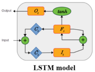
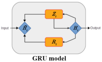
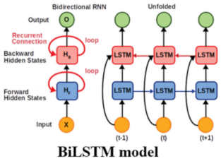
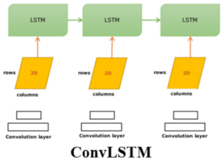
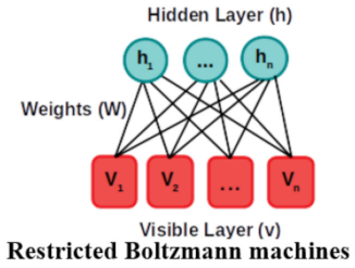
Deep learning techniques, which possess good capabilities in automatically learning pertinent features embed in data, are examined in this study to forecast PV power output. Table 1, summarizes the pros and cons of the seven considered benchmark deep learning architectures: RNN [39], LSTM [40], GRU [41], Bi-LSTM [42], ConvLSTM [43], SAE [44], RBM [45,46], and VAE [20,47].

Variational Autoencoders Model

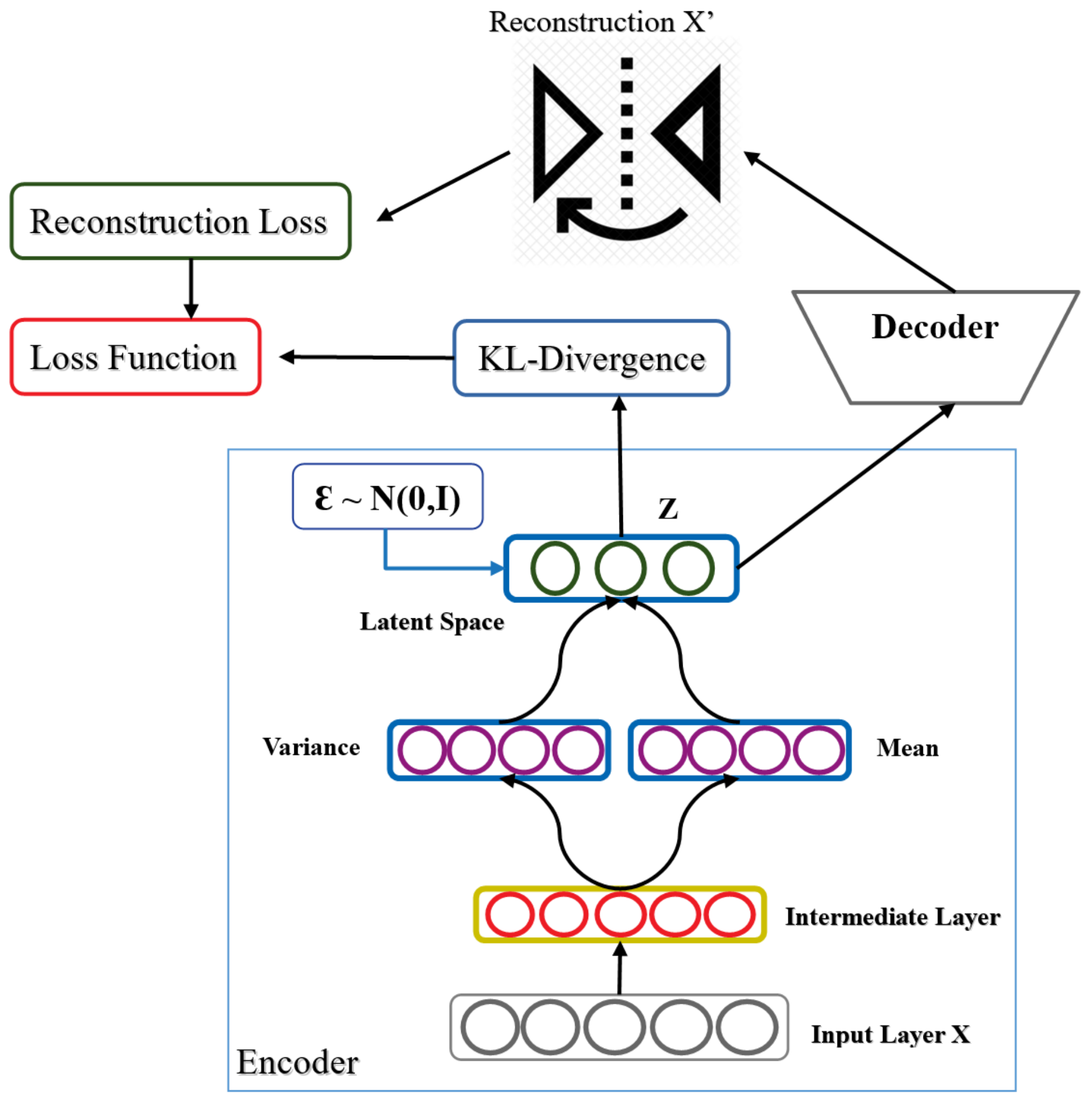
VAEs are an essential class of generative-based techniques that are efficient to automatically extract information from data in an unsupervised manner [20,47]. One desirable characteristic of VAEs is their ability for reducing the input dimensionality enabling them to compress large dimensional data into a compressed representation. Moreover, they are very effective for approximating complex data distributions using stochastic gradient descent [47]. There are two major advantages of VAEs compared the conventional autoencoders, one is they are efficient to solve the overfitting problem in the conventional autoencoders by using a regulation mechanism in the training phase, and the second advantage is that they have proved effective when handling various kinds of complex data in different applications, including handwritten digits, and urban networks modeling [48]. Here, VAE is adopted for solar PV production forecasting. Figure 1 shows a schematic diagram of the construction of a VAE.
Basically, the VAE, as a variant of autoencoders, contains two neural networks an encoder and a decoder, where the encoder mission is to encode a given observed set, X into a latent space Z as distribution, q z | x . The latent (termed hidden) space dimension is decreased in comparison to the dimension of the observed set. Indeed, the encoder is built to compress the observed set toward this reduced dimensional space efficiently. Then, a sample is generated via, z q ( z | x ) ,using the learned probability distribution. On the other hand, the key purpose of the decoder, p x | z , consists in generating the observation x based on the input z. It should be emphasized that the reconstruction of data using the decoder results in some deviation of reconstruction, which is calculated and backpropagated through the network. This error is minimized in the training phase of the VAE model by the minimization of the deviation between the observed set and the encoded-decoded set.
To summarize, the VAE encoder is gotten via an approximate posterior q θ z | x , and the decoder is obtained by a likelihood p ϕ x | z , where θ and ϕ refers respectively to the parameters of encoder and decoder. Here a neural network is constructed for learning θ and ϕ . Essentially, the VAE encoder’s role is learning latent variable z based on gathered sensor data, and the decoder employs the learned latent variable z for recovering the input data. The deviation between the reconstructed data and the input data should be close to zero as possible. Notably, the learned latent variable z from the encoder is used for feature extraction based on the input data. Usually, the dimension of the output of the encoder is smaller than that of the original data, which leads to the dimensionality reduction of input data. Note that the encoder is trained by training the entire VAE comprising encoder and decoder.
It is worth pointing out that the loss function has an essential effect on feature extraction for training VAE. Assume that X t = [ x 11 , x 2 t , , x N t ] is the input data points of VAE at time point t, and X t is the reconstructed data using the VAE model. Furthermore, it is assumed maximizing the marginal likelihood learning of parameters, expressed as [49]:
l o g p ϕ ( x ) = D K L [ q θ ( z | x ) p ϕ ( x ) ] + L ( θ , ϕ ; x ) ,
where D K L [ . ] denotes the Kulback-Leibler divergence, and L refers to the likelihood of the parameters of encoder and decoder (i.e., θ and ϕ ). Hence, the loss can be expressed as
L ( θ , ϕ ) = E z q θ ( z | x ) l o g p ( x | z ) Reconstruction term D K L q θ ( z | x ) | | p ϕ ( z ) Regularization term .
The VAE’s loss function is composed of two parts: the reconstruction loss and a regularizer. Reconstruction loss tries to get an efficient encoding-decoding procedure. In contrast, a regularizer part permits the regularization of the latent space construction to approximate the distributions out of the encoder as near as feasible to a prefixed distribution (e.g., Normal distribution). Figure 2 schematically summarizes the procedure for computing the loss function.
The term (2) permits reinforcing the decoder capacity to learn data reconstruction. Higher values of the reconstruction loss mean that the performed reconstruction is not suitable, while lower values mean that the model is converging. The regularizer is reported using the Kulback-Leibler (KL) divergence separating the distribution of the encoder function ( q θ ( z | x ) ) and of the latent variable prior ( z , | p ϕ ( z ) ). Indeed, KL is employed to compute the distance that separates two given probability distributions. The gradient descent method is used to minimize the loss function with respect to the encoder’s parameters and decoder in the training phase. Overall, we minimize the loss function to ensure getting a regular latent space, z, and adequate sampling of new observation using z p ϕ ( z ) [50].
Let assume that p ϕ ( z ) = N ( z ; 0 , I ) , we can write q θ ( z | x ) in the following form:
l o g q θ ( z | x ) = l o g N ( z ; μ , σ 2 I ) .
The mean and standard deviation of the approximate posterior are denoted by ( μ , σ ), respectively. Note here that a layer is dedicated to both of them. Moreover, the latent space z is constructed using a deterministic function g parameterized by ϕ and an auxiliary noise variable ε p ( ε ) or more specifically ε N ( 0 , I ) .
z = g ϕ ( x , ε ) = μ + σ ε .
The reconstruction error term can be expressed in the following form:
L ( θ , ϕ , x ) = 1 2 i 1 + l o g ( ( σ i ) 2 ) ( μ i ) 2 ( σ i ) 2 + 1 L l = 1 L l o g ( p ϕ ( x | z ( l ) ) ) ,
where the ⊙ denotes the element-wise product.
Overall, the encoder and decoder’s parameters are obtained by minimizing the loss function, L ( θ , ϕ ) , using the training observations. The VAE is trained using the procedure tabulated Algorithm 1.
Algorithm 1: VAE training algorithm.
Applsci 10 08400 i008

3. Deep Learning-Based PV Power Forecasting

The input data consists of PV power output that variates between 0 and the rated output power. Thus, when handling some large-value data with the RNN model, a gradient explosion can be occurred and negatively affects the performance of the RNN. Furthermore, the learning effectiveness of RNN will be reduced. To remedy this issue, the input data is normalized via min-max normalization within the interval [ 0 , 1 ] , and then used for constructing the deep learning models. The normalization of the original measurements, y is defined as:
y ˜ = ( y y m i n ) ( y m a x y m i n ) ,
where y m i n and y m a x refer to the minimum and maximum of the raw PV power data, respectively. After getting forecasting outputs, we applied a reverse operation to ensure that the forecasted data match to the original PV power time-series data.
y = y ˜ ( y m a x y m i n ) + y m i n .
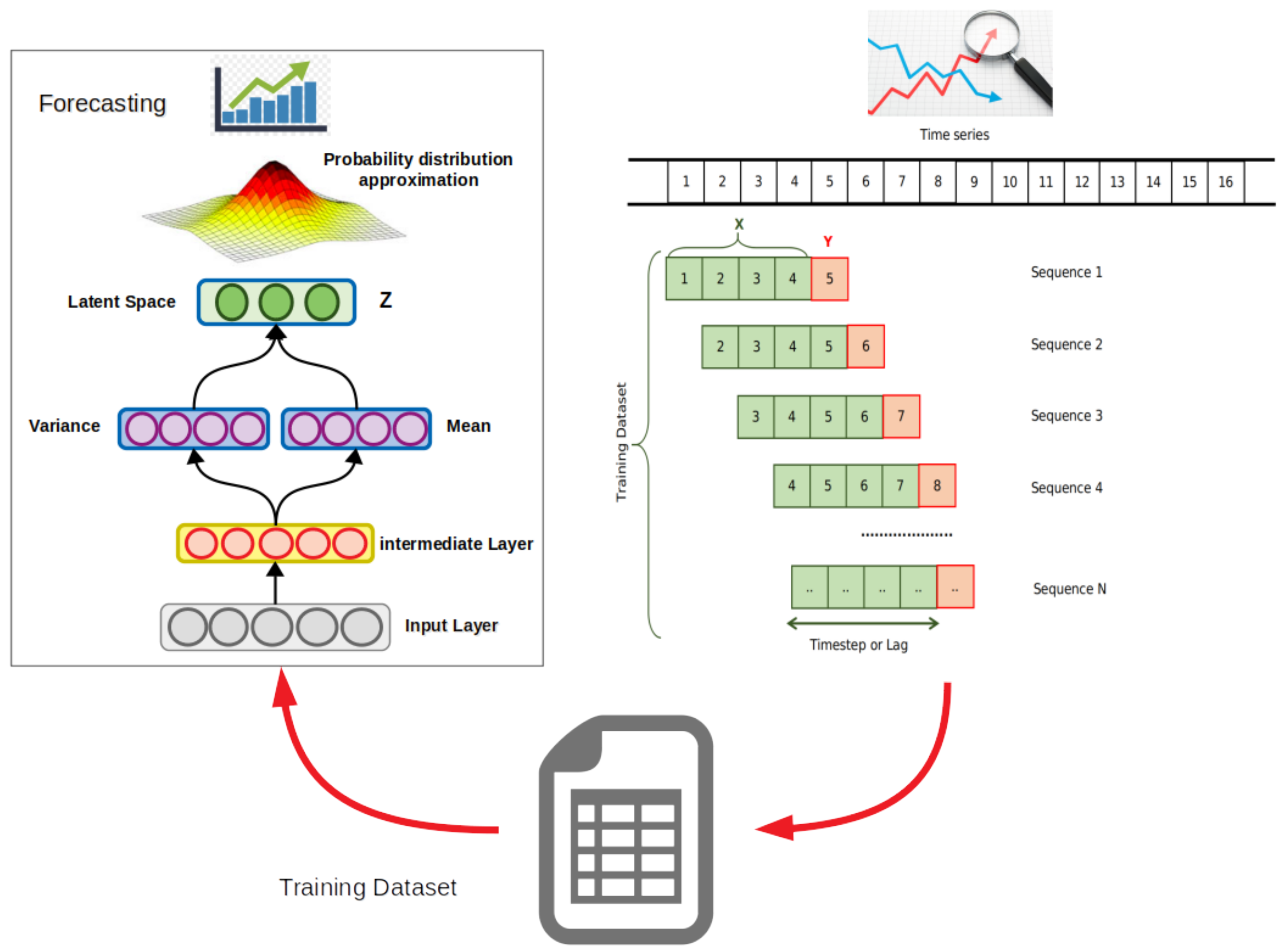
As discussed above, the generated PV power shows a high level of variability and volatility because of its high correlation with the weather conditions. Hence, for mitigating the influence of uncertainty on the accuracy of the PV power forecasting this work presents a deep-learning framework to forecast PV power output time-series. Essentially, deep learning models are an efficient tool to learn relevant features and process nonlinearity from complex datasets. In this study, a set of eight deep learning models have been investigated and compared for one-step and multiple steps ahead forecasting of solar PV power. The overall structure of the proposed forecasting procedures is depicted in Figure 3. As shown in Figure 3, solar PV power forecasting is accomplished in two phases: training and testing. The original PV power data is split into a training sub-data and a testing sub-data. At first, the raw data is normalized to build deep learning models. Adam optimizer is used to select the values of parameters of each model by minimizing the loss function based on training data. Once the models are constructed, they are exploited for PV power output forecasting. The quality of models are quantified using several statistical indexes including the Coefficient of determination ( R 2 ), explained variance (EV), mean absolute error (MAE), Root Mean Square Error (RMSE), and normalized RMSE (NRMSE).
Essentially, the deep learning-driven forecasting methods learn the temporal correlation hidden on the PV power output data and expected to uncover and captures the sequential features in the PV power time series. The main objective of this study is to investigate the capability of learning models namely RNN, LSTM, BiLSTM, ConvLSTM, GRU, RBM, SAE, and VAE for one-step and multiple-steps ahead solar PV power forecasting.

3.1. Training Procedure

The eight models investigated in this study can be categorized into two classes: autoencoders and recurrent neural networks. The autoencoders represented include RBM, VAE, and SAEs while the RNN-based models contain RNN, LSTM, GRU, BiLSTM, and ConvLSTM. The dataset used for training and testing are normalized first, and more data preprocessing is needed for the autoencoder models. For instance, data reshaping is needed to transform the univariate PV power time-series data to a two-dimension matrix to be used as input for the autoencoders including the SAE, VAE, and RBM. The main difference between the two classes in the training phase is the learning way, the RNNs are entirely supervised trained while the auto-encoders are first pre-trained in an unsupervised manner and then the training is completed based on supervised learning. Specifically, RNNs models are trained in a supervised way by using a subset of training as input sequence ( X = x 1 , , x k ) and an output variable Y = x k + 1 . The sequence length l, called the lag, is a crucial parameter used in the data preparation phase. The mapping sequence to the next value is constructed using a window sliding algorithm. The value of l is determined using the Grid Search approach [51]. Here, the value of l is chosen 6, which is the lowest value that maximizes the overall performance of the proposed approach.
RNN—based models are trained to learn the mapping function from the input to the output. After that, these trained models are used to forecast new data that complete the sequence. On the other hand, the greedy layer-wise unsupervised plus fine-tuning were applied to RBM, VAE, and SAES. It should be noted that PV power output forecasting based on autoencoder is accomplished as a dimensionality reduction. That is these models do not have the possibility to discover time dependencies or model time series data. Hinton [44] shows that a greedy layerwise unsupervised learning for each layer followed by a fine-tuning improves the features extraction and learning process of the neural networks dedicated to prediction problems or for dimensionality reduction like autoencoders. The VAE-driven forecasting procedure including the pretreatment step is illustrated in Figure 4.

3.2. Measurements of Effectiveness

The deep learning-driven forecasting methods will be evaluated using the following metrics: R 2 , RMSE, MAE, EV, and NRMSE.
R 2 = i = 1 n [ ( y i , y ¯ ) · ( y ^ i y ^ ¯ ) ] 2 i = 1 n ( y i y ¯ ) 2 · i = 1 n ( y ^ i y ^ ¯ ) 2 ,
R M S E = 1 n t = 1 n ( y t y ^ t ) 2 ,
M A E = t = 1 n y t y ^ t n ,
E V = 1 Var ( y ^ y ) Var ( y ) ,
N R M S E = 1 i = 1 N ( y i y ^ ) 2 i = 1 N ( y i y ¯ ) 2 . 100 % ,
where y t are the actual values, y ^ t are the corresponding estimated values, y ¯ is the mean of measured power data points, and n is the number of measurements. Instead of using RMSE that relies on the range of the measured values, the benefit of using NRMSE as the statistical indicator is that it does not rely on the range of the measured values. NRMSE metric indicates how well the forecasted model response matches the measurement data. A value of 100% for NRMSE denotes perfect forecasting and lower values characterize the poor forecasting performance. Lower RMSE and MAE values and EV and R2 closer to 1 are an indicator of accurate forecasting.

4. Results and Discussion

4.1. Data Description

In this study, solar PV power data from two PV systems are adopted to verify the performance of the eight deep learning-driven forecasting methods.
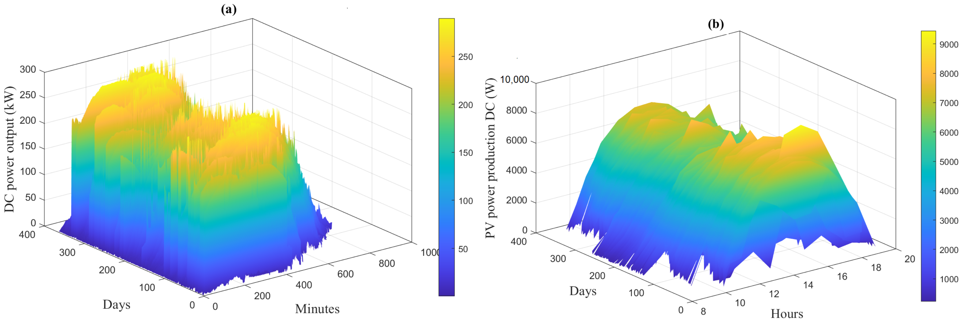
  • Data Set 1: The first historical solar-PV power dataset used are collected from a parking lot canopy array monitored by the National Institute of Standard and Technology (NIST) [52]. The PV system contains eight canopies tilted 5 degrees down from horizontal, four canopies tilt to the west, and the other four canopies tilt to the east. The modules are installed with their longer dimension running east-west. Each shed contains 129 modules laid out in a 3 (E − W) × 43 (N − S) grid. This power system has a rated DC power output of 243 kW. The first dataset is collected from January 2015 to December 2017 with a one-minute temporal resolution. The distribution of the Parking Lot Canopy Array dataset collected from January 2015 to December 2015 are shown in Figure 5a.
  • Data Set 2: The second solar-PV power dataset is collected from a grid-connected plant in Algeria with a peak power of 9 MWp from January 2018 to December 2018 with 15 min temporal resolution. This PV plant consists of nine identical mini-PV plants of one mega each. Indeed, a set of 93 PV array provides one MWp of DC power, two central inverters with 500 kVA each, allow to connect the 93 PV array to one transformer of 1250 kVA. The hourly distribution of the first dataset are shown in Figure 5b.
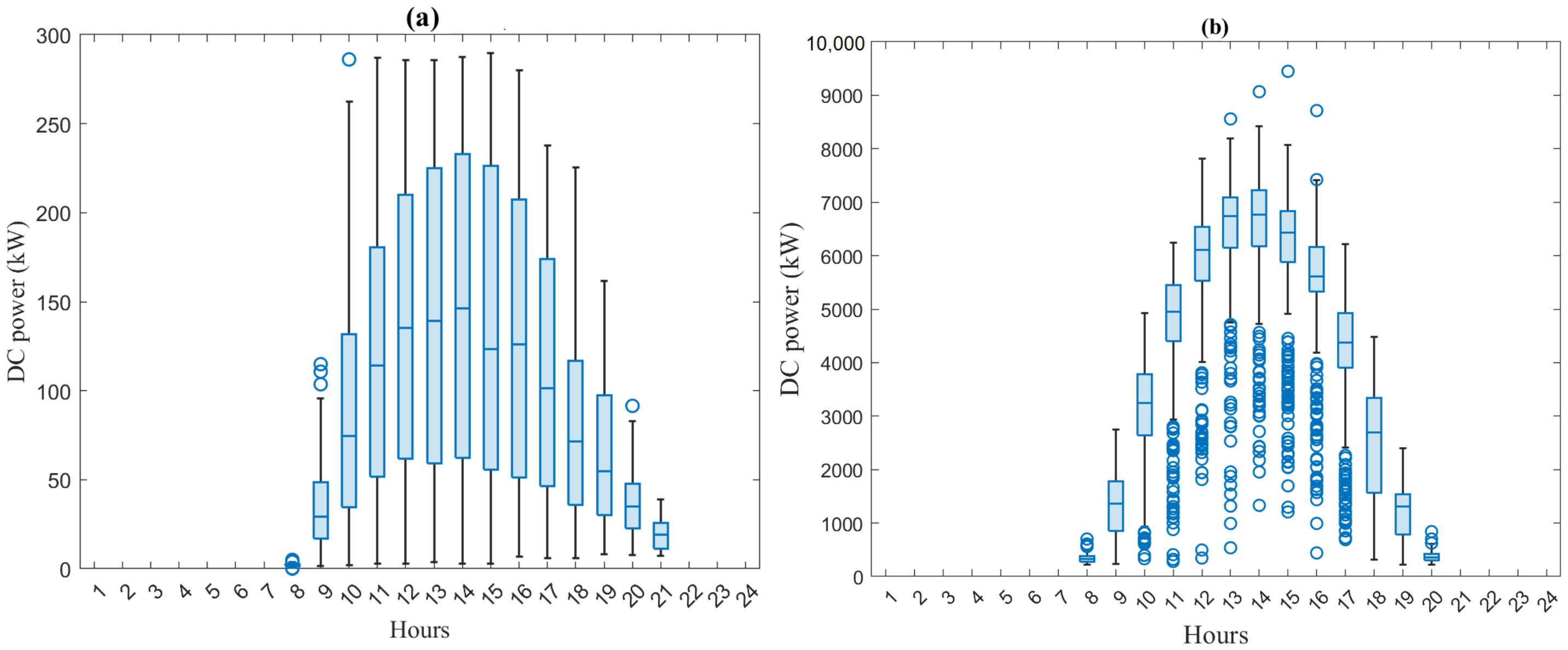
Figure 6 depicts the boxplots of DC power output (Data Set 1 and Data Set 2) in Figure 5 to show the distribution of DC power in the daytime. The maximum power is generated around mid-day.

4.2. Forecasting Results

Accurate short-term forecasting of PV power output gives pertinent information for maintaining the desired power grid production delivery and storage [7,53]. This section assesses the eight models (i.e., RNN, GRU, LSTM, BiLSTM, ConvLSTM, RBM, AE, and VAE) and compares their forecasting performance using PV power output collected from two different PV systems. Towards this ends, we first build each to capture the maximum variance in training data and then use them to forecast the future trend of PV power output. The training data in Data Set 1 consists of one-minute power data collected from 1 January 2017 to 29 June 2017. The training data in Data Set 2 is collected from 1 January 2018 to 19 October 2018. The hyper-parameters of the built deep learning methods based on training datasets are tabulated in Table 2. For all models, we used the cross-entropy as loss function and Rmsprop as an optimizer in training.

4.2.1. Forecasting Results Based on Data Set 1: Parking Lot Canopy Array Datasets

The principal feature of the PV power output is its intermittency. This unpredicted fluctuation in solar PV power could lead to many challenges including power generation control and storage management. Essentially, it is crucial to appropriately forecast PV power output to guarantee reliable operation and economic integration in the power grid. In the first case study, the above-trained models will be evaluated using the testing solar PV power output starting from 30 June to 6 July 2017 collected from Parking lot canopy array. Forecasting outputs using the eight deep learning models using test measurements are displayed in Figure 7. These results illustrate the goodness of deep learning models for PV power forecasting.
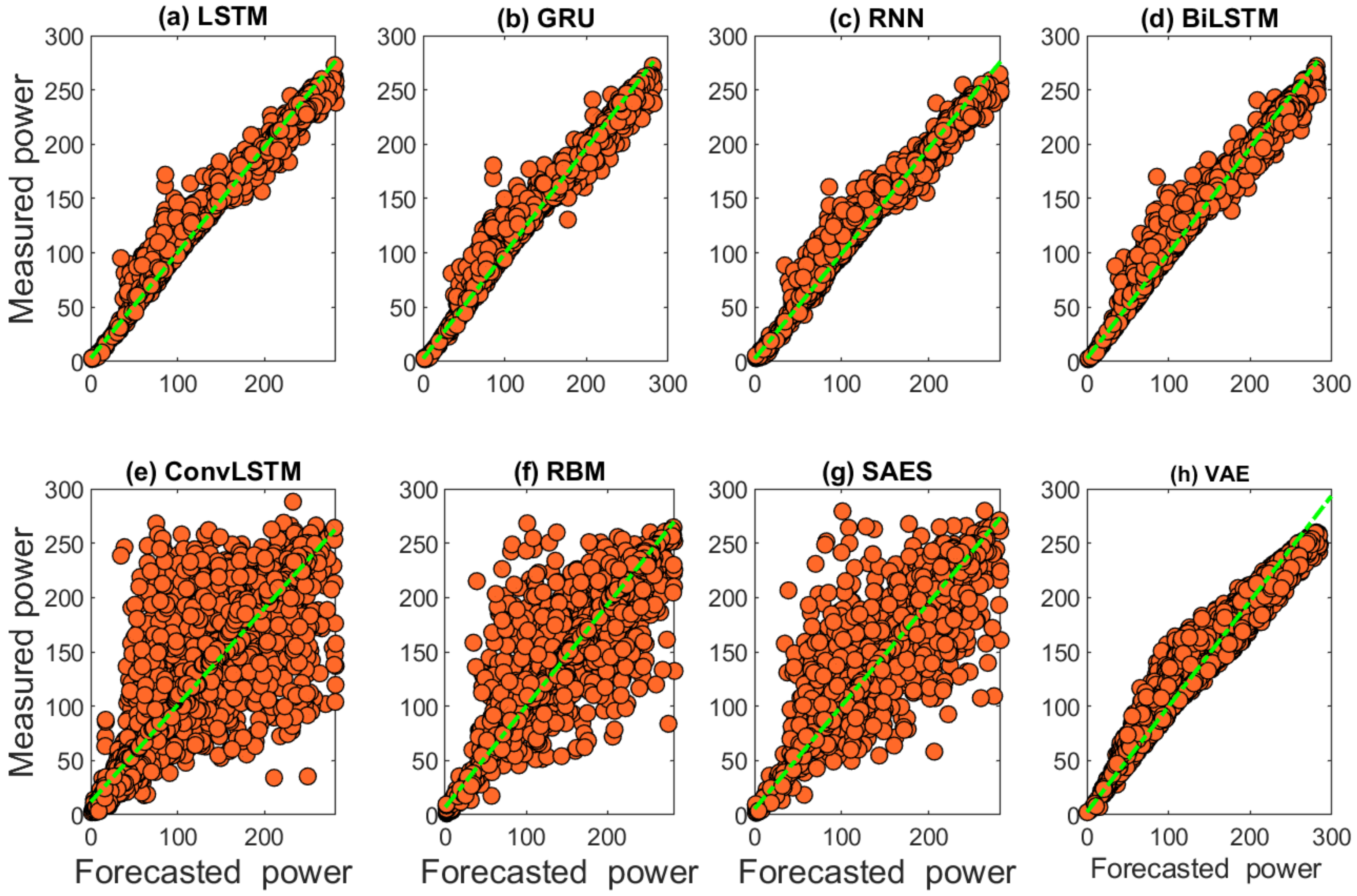
Also, to show clearly the accordance of the measured and the forecast outputs from the investigated deep learning models, the scatter plots are presented in Figure 8. Figure 8 shows that the forecasted data from RBM and SAE models are moderately correlated with the actual PV power output. The forecasting with ConvLSTM is relatively weakly correlated with the measured power data. On the other hand, the forecasted power with RNN-based models and the VAE model are strongly correlated with the measured PV power.
Now, to quantitatively evaluate the forecasting accuracy of the eight considered models based on the testing data, five statistical indexes are computed and listed in Table 3. Also, we compared the eight the forecasting results of the ten deep learning models with two baseline machine learning models: LR and SVR (Table 3). For this application, ConvLSTM performs poorly in terms of the forecasting accuracy compared to the other models and cannot track well the variability of PV power and does not describe the most variance in the data (i.e., EV = 0.832). Moderate forecasting performance are obtained using RBM and SAE by explaining respectively 0.929 and 0.932 of the total variance in the testing PV power data. The results of this investigation exhibit also that the VAE model provides accurate forecast in comparison to the other models by achieving PV power forecast with lower RMSE, MAE, and higher NRMSE (%) as well as the highest R2, EV values closer to 1 that means that most of the variance in the data is captured by the VAE model. Specifically, the VAE model achieved the highest R2 of 0.992 and the lower RMSE (6.891) and MAE (5.595). We highlight that this is the first time that the VAE model is used for solar PV power output forecasting. This application showed that the VAE method for PV power forecasting has superior performance. Also, it is noticed that RNN and its extended variants LSTM, BiLSTM, and GRU achieve slightly comparable performance to the VAE in terms of the statistical indexes (RMSE, RMSE, MAE, EV, and NRMSE). Table 3 indicates that deep learning models exhibited improved forecasting performance compared to the baseline methods (i.e., LR and SVR).

4.2.2. Forecasting Results Based on Data Set 2: Algerian PV Array Datasets

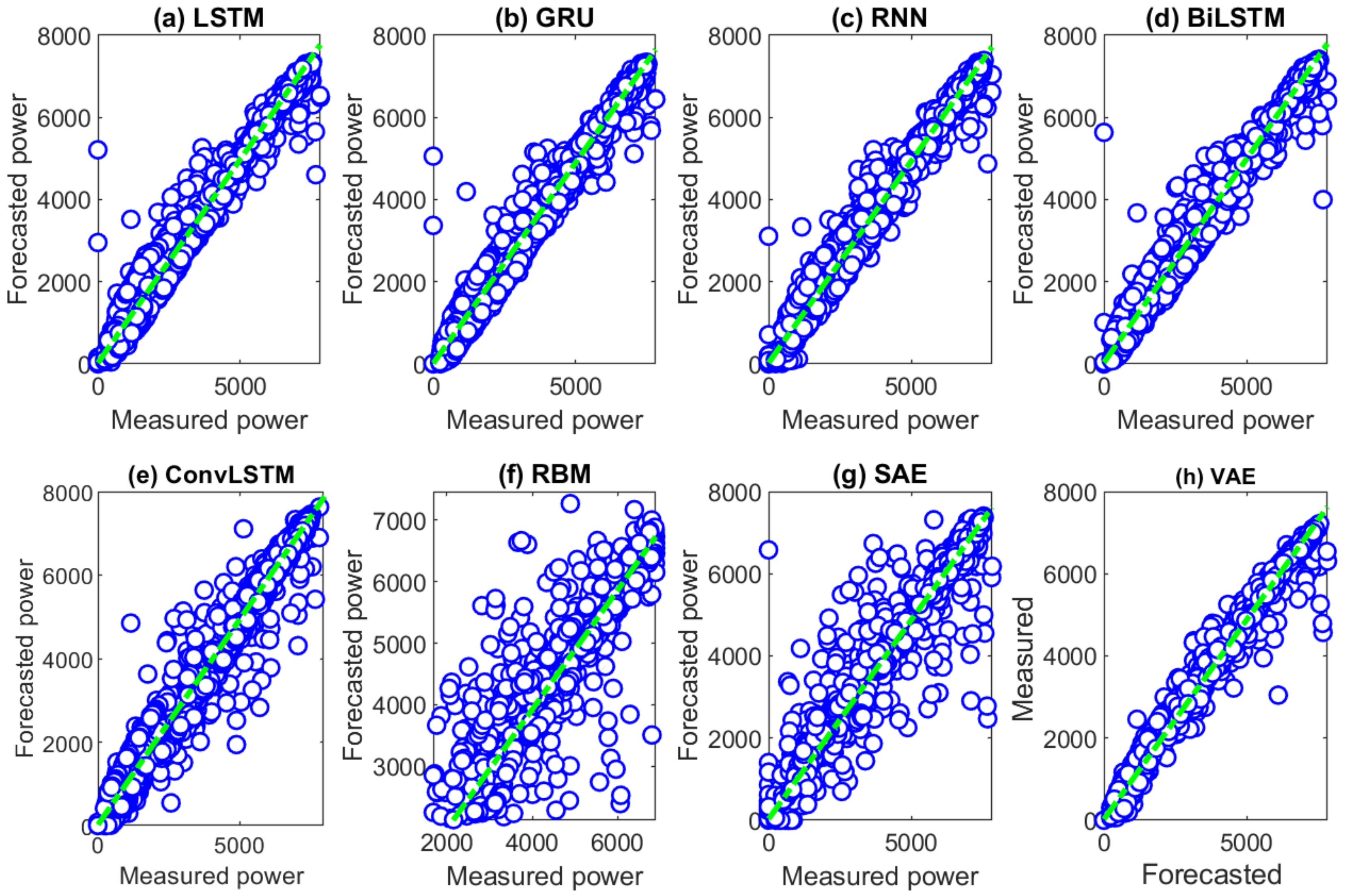
Now, the effectiveness of the eight methods will be tested based on power output data collected from the 9 MWp PV plant in Algeria (Data Set 2). In this experiment, the above-trained models will be evaluated using the testing solar PV power output collected from 20 October to 31 December 2018. The measured test set together with model forecasts are charted in Figure 9. Similar conclusions are also valid for these datasets. One major reason is that RNN-based models have a strong capability to describe time dependents data and can better model the complicated relationship between historical and future PV power output data than other methods. The RNN-based models and the VAE model again confirm the superior forecasting performance of PV power output as shown by the scatter plots in Figure 9. The ConvLSTM model shows poor forecasting performance results (Figure 9).
And then, the statistical indicators are computed to compare the forecasting performance between the eight models, and baseline machine learning models: LR and SVR based on testing datasets (Table 4). It is worth noting that the RNN-based models (i.e., RNN, LSTM, BiLSTM, ConvLSTM, and GRU) and the VAE model show the improved forecasting performance compared to the RBM, and SAE.
Results in Figure 9 and Table 4 indicate that using RNN-based models and VAE method has led to improved forecasting performance. Furthermore, the error analysis highlights that the forecasting accuracy obtained by these models can satisfy practical needs and can be useful for PV power management. It should be noted that the VAE model is trained in an unsupervised manner in order to forecast solar PV power. This means that the forecast is based only on the information from past data. However, the other models are trained in a supervised way by using a subset of training as input sequence ( x 1 , , x k ) and an output variable x k and we train RNN-based models to learn the mapping function from the input to the output. After that, these trained models are used to forecast new data. Even if the VAE model is trained in an unsupervised way, it can provide comparable forecasting performance to those obtained by the supervised RNN-based models. Accordingly, the VAE-based forecasting approach is a more flexible and powerful tool to be used in real-time PV power forecasting.
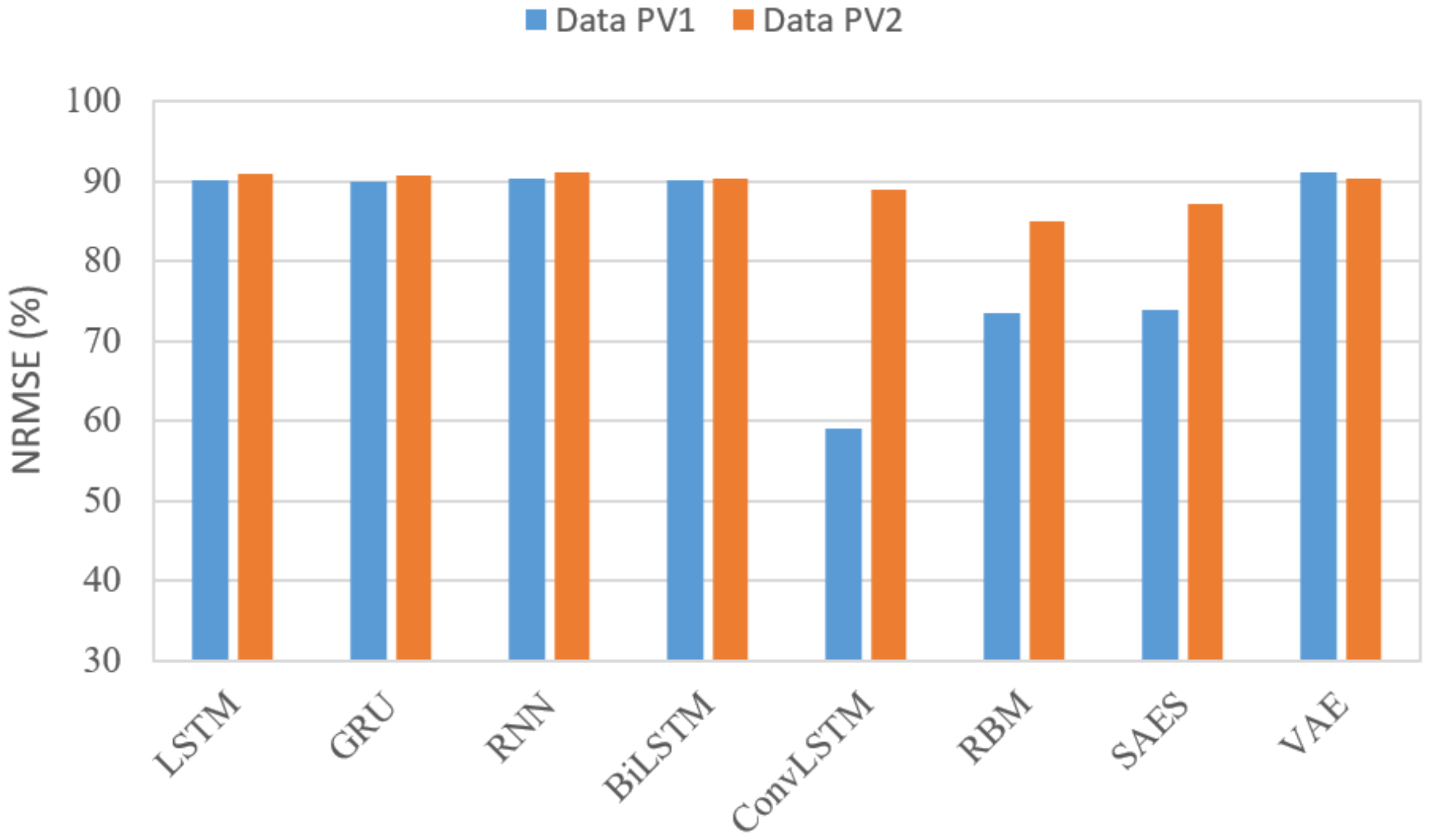
Overall, the NRMSE (%) quantifies the quality of power forecasting between the measured and forecasted PV power output time-series data, where the larger value indicates a better prediction performance. A visual display of the NRMSE (%) derived with the eight considered deep learning methods based on the testing datasets from the two PV systems is displayed in Figure 10. The first dataset is with a one-minute resolution and the second dataset is with fifteen minutes resolution. The VAE model achieves better PV power flow forecast performance compared to the RBM and SAE models and RNN-based models. Furthermore, the results show that VAE models are efficient in capturing the linear and nonlinear features in PV power data with different time resolutions.

4.3. Multi-Step Ahead PV Power Forecasts

Precise multi-step forecasts are essential to managing the operation of PV systems appropriately. Now, we assess the capability of the eight methods for multi-step ahead forecasting of PV power output using data from Data Set 1 (a 243 kW parking lot canopy array in the US) and Data Set 2 (a 9 MW PV system in Algeria). Based on the past measurements, x = [ x 1 , x 2 , , x l ] , the computed single-, two-, and multistep-ahead forecast are respectively x l + 1 , x l + 2 , and x l + n . The 5, 10, 15 steps-ahead forecastings of PV power data based on the testing data of the Parking lot canopy array dataset and the Adrar PV system are tabulated in Table 5.
We can easily observe that, for all data sets, except BiLSTM and ConvLSTM, the other models performed consistently reasonable forecasting results five-, ten-, fifteen-step-ahead forecasting. For instance, the VAE model achieved R2 values of 0.902,0.873, 0.856 for five-, ten-, fifteen-step-ahead forecasting when using the first for Data Set 1, R2 values of 0.951,0.877, 0.818 for Data Set 2. The RNN, GRU, RBM, SAE, and VAE models performed about equally in terms of R2, MAPE, and RMSE in all cases.
For Data Set 1, the five-step-ahead forecasting R2’s for all models except ConvLSTM is around 0.90 (Table 5). Results in Table 5 show that for five-steps ahead forecasting based Data Set 2 almost all models provide relatively good forecasting accuracy in terms of R 2 which is around 0.94 . It is worthwhile noticing that for a ten-step -ahead forecast, the accuracy of all models starts to decrease and achieve R 2 values around 0.86 . In the fifteen-step -ahead forecasting, we observed that LSTM, BiLSTM, and ConvLSTM achieved poor forecasting performance. The other models are still providing acceptable forecasting accuracy. We notice that the SAE model outperforms slightly the other models with higher R 2 and lowest forecasting errors. The overall forecasting performance of the RNN, GRU, RBM, SAE, and VAE model was satisfying, and they can maintain a reasonable forecasting performance to forecast solar PV power output as the number of steps increases. The error for the second dataset is large compared to the first one. The first dataset is 15 min time resolution recorded for one year, while the second data is of one-minute time resolution recorded for three years. Moreover, we used 90% of data for both datasets for training and 10% for testing. The one-minute data is very dynamic, which explains the large error compared to the first dataset.
It is challenging to tell which models were absolutely superior on the basis of the R2, MAPE, and RMSE values. The results of this study show that RNN, GRU, and VAE performs slightly better on average than the other models in most cases for one- and multi-step-ahead forecasting. The obtained results demonstrate that both RNNs with supervised learning and VAE with unsupervised learning can perform a one-step and multi-step forecasting accurately. Overall, the VAE deep learning model gives an effective way to model and forecast PV power output, and it has emerged as a serious competitor to the RNN-driven models (i.e., RNN, GRU, and LSTM).

5. Conclusions

PV power output possesses high volatility and intermittency because of its great dependency on environmental factors. Hence, a reliable forecast of solar PV power output is indispensable for efficient operations of energy management systems. This paper compares eight deep learning-driven forecasting methods for solar PV power output modeling and forecasting. The considered models can be categorized into two categories: supervised deep learning methods, including RNN, LSTM, BiLSTM, GRU, and ConvLSTM, and unsupervised methods, including AE, VAE, and RBM. We also compared the performance of the deep learning methods with two baseline machine learning models (i.e., LR and SVR). It is worth highlighting that this study introduced the VAE and RBM methods to forecast PV power. For efficiently managing the PV system, both single- and multi-step-ahead forecasts are considered. The forecasting accuracy of the ten models has been evaluated using two real-world datasets collected from two different PV systems. Results show the domination of the VAE-based forecasting methods due to its ability to learn higher-level features that permit good forecasting accuracy.
To further enhance the forecasting performance, in future study, we plan to consider multivariate forecasting by incorporating weather data. Also, these deep learning models can be applied and compared using data from other renewable energy systems, such as forecasting the power generated by wind turbines. Further, it will be interesting to conduct comparative studies to investigate the impacts of data from different technologies, such as monocrystalline, and polycrystalline.

Author Contributions

A.D.: Conceptualization, Formal analysis, Investigation, Methodology, Software, Writing-original draft, Writing-review & editing F.H.: Conceptualization, Formal analysis, Investigation, Methodology, Software, Supervision, Writing-original draft, Writing-review & editing Y.S.: Investigation, Conceptualization, Formal analysis, Methodology, Writing-review & editing, Funding acquisition, Supervision. S.K.: Investigation, Conceptualization, Formal analysis, Methodology, Writing- original draft. All authors have read and agreed to the published version of the manuscript.

Funding

This work was supported by funding from King Abdullah University of Science and Technology (KAUST), Office of Sponsored Research (OSR) under Award No: OSR-2019-CRG7-3800.

Conflicts of Interest

The authors declare no conflict of interest.

References

  1. Masa-Bote, D.; Castillo-Cagigal, M.; Matallanas, E.; Caamaño-Martín, E.; Gutiérrez, A.; Monasterio-Huelín, F.; Jiménez-Leube, J. Improving photovoltaics grid integration through short time forecasting and self-consumption. Appl. Energy 2014, 125, 103–113. [Google Scholar] [CrossRef] [Green Version]
  2. Behera, M.K.; Majumder, I.; Nayak, N. Solar photovoltaic power forecasting using optimized modified extreme learning machine technique. Eng. Sci. Technol. Int. J. 2018, 21, 428–438. [Google Scholar] [CrossRef]
  3. Wang, K.; Qi, X.; Liu, H. A comparison of day-ahead photovoltaic power forecasting models based on deep learning neural network. Appl. Energy 2019, 251, 113315. [Google Scholar] [CrossRef]
  4. Harrou, F.; Kadri, F.; Sun, Y. Forecasting of Photovoltaic Solar Power Production Using LSTM Approach. In Advanced Statistical Modeling, Forecasting, and Fault Detection in Renewable Energy Systems; IntechOpen: London, UK, 2020. [Google Scholar]
  5. Fu, M.P.; Ma, H.W.; Mao, J.R. Short-term photovoltaic power forecasting based on similar days and least square support vector machine. Power Syst. Prot. Control 2012, 40, 65–69. [Google Scholar]
  6. Sun, M.; Feng, C.; Zhang, J. Probabilistic solar power forecasting based on weather scenario generation. Appl. Energy 2020, 266, 114823. [Google Scholar] [CrossRef]
  7. Qing, X.; Niu, Y. Hourly day-ahead solar irradiance prediction using weather forecasts by LSTM. Energy 2018, 148, 461–468. [Google Scholar] [CrossRef]
  8. Chitalia, G.; Pipattanasomporn, M.; Garg, V.; Rahman, S. Robust short-term electrical load forecasting framework for commercial buildings using deep recurrent neural networks. Appl. Energy 2020, 278, 115410. [Google Scholar] [CrossRef]
  9. Li, P.; Zhou, K.; Lu, X.; Yang, S. A hybrid deep learning model for short-term PV power forecasting. Appl. Energy 2020, 259, 114216. [Google Scholar] [CrossRef]
  10. Kanchana, W.; Sirisukprasert, S. PV Power Forecasting with Holt-Winters Method. In Proceedings of the 2020 8th International Electrical Engineering Congress (iEECON), Chiang Mai, Thailand, 4–6 March 2020; pp. 1–4. [Google Scholar]
  11. Prema, V.; Rao, K.U. Development of statistical time series models for solar power prediction. Renew. Energy 2015, 83, 100–109. [Google Scholar] [CrossRef]
  12. Kushwaha, V.; Pindoriya, N.M. A SARIMA-RVFL hybrid model assisted by wavelet decomposition for very short-term solar PV power generation forecast. Renew. Energy 2019, 140, 124–139. [Google Scholar] [CrossRef]
  13. Lin, K.P.; Pai, P.F. Solar power output forecasting using evolutionary seasonal decomposition least-square support vector regression. J. Clean. Prod. 2016, 134, 456–462. [Google Scholar] [CrossRef]
  14. Zhang, G.; Guo, J. A Novel Method for Hourly Electricity Demand Forecasting. IEEE Trans. Power Syst. 2020, 35, 1351–1363. [Google Scholar] [CrossRef]
  15. Sanjari, M.J.; Gooi, H.B.; Nair, N.C. Power Generation Forecast of Hybrid PV—Wind System. IEEE Trans. Sustain. Energy 2020, 11, 703–712. [Google Scholar] [CrossRef]
  16. Rana, M.; Rahman, A. Multiple steps ahead solar photovoltaic power forecasting based on univariate machine learning models and data re-sampling. Sustain. Energy Grids Netw. 2020, 21, 100286. [Google Scholar] [CrossRef]
  17. Andrade, J.R.; Bessa, R.J. Improving Renewable Energy Forecasting With a Grid of Numerical Weather Predictions. IEEE Trans. Sustain. Energy 2017, 8, 1571–1580. [Google Scholar] [CrossRef] [Green Version]
  18. Su, H.; Liu, T.; Hong, H. Adaptive Residual Compensation Ensemble Models for Improving Solar Energy Generation Forecasting. IEEE Trans. Sustain. Energy 2020, 11, 1103–1105. [Google Scholar] [CrossRef]
  19. Zhang, X.; Li, Y.; Lu, S.; Hamann, H.F.; Hodge, B.; Lehman, B. A Solar Time Based Analog Ensemble Method for Regional Solar Power Forecasting. IEEE Trans. Sustain. Energy 2019, 10, 268–279. [Google Scholar] [CrossRef]
  20. Harrou, F.; Sun, Y.; Hering, A.S.; Madakyaru, M.; Dairi, A. Statistical Process Monitoring Using Advanced Data-Driven and Deep Learning Approaches: Theory and Practical Applications; Elsevier: Amsterdam, The Netherlands, 2020. [Google Scholar]
  21. Dairi, A.; Cheng, T.; Harrou, F.; Sun, Y.; Leiknes, T. Deep learning approach for sustainable WWTP operation: A case study on data-driven influent conditions monitoring. Sustain. Cities Soc. 2019, 50, 101670. [Google Scholar] [CrossRef]
  22. Harrou, F.; Dairi, A.; Sun, Y.; Kadri, F. Detecting abnormal ozone measurements with a deep learning-based strategy. IEEE Sens. J. 2018, 18, 7222–7232. [Google Scholar] [CrossRef] [Green Version]
  23. Harrou, F.; Dairi, A.; Sun, Y.; Senouci, M. Statistical monitoring of a wastewater treatment plant: A case study. J. Environ. Manag. 2018, 223, 807–814. [Google Scholar] [CrossRef]
  24. Dairi, A.; Harrou, F.; Sun, Y.; Senouci, M. Obstacle detection for intelligent transportation systems using deep stacked autoencoder and k-nearest neighbor scheme. IEEE Sens. J. 2018, 18, 5122–5132. [Google Scholar] [CrossRef] [Green Version]
  25. Krizhevsky, A.; Sutskever, I.; Hinton, G.E. ImageNet Classification with Deep Convolutional Neural Networks. In Advances in Neural Information Processing Systems 25; Pereira, F., Burges, C.J.C., Bottou, L., Weinberger, K.Q., Eds.; Curran Associates, Inc.: New York, NY, USA, 2012; pp. 1097–1105. [Google Scholar]
  26. Young, T.; Hazarika, D.; Poria, S.; Cambria, E. Recent trends in deep learning based natural language processing. IEEE Comput. Intell. Mag. 2018, 13, 55–75. [Google Scholar] [CrossRef]
  27. Graves, A.; Rahman Mohamed, A.; Hinton, G.E. Speech Recognition with Deep Recurrent Neural Networks. In Proceedings of the 2013 IEEE International Conference on Acoustics, Speech and Signal Processing, Vancouver, BC, Canada, 26–31 May 2013. [Google Scholar]
  28. Zeroual, A.; Harrou, F.; Dairi, A.; Sun, Y. Deep learning methods for forecasting COVID-19 time-Series data: A Comparative study. Chaos Solitons Fractals 2020, 140, 110121. [Google Scholar] [CrossRef] [PubMed]
  29. Harrou, F.; Hittawe, M.M.; Sun, Y.; Beya, O. Malicious attacks detection in crowded areas using deep learning-based approach. IEEE Instrum. Meas. Mag. 2020, 23, 57–62. [Google Scholar] [CrossRef]
  30. Hittawe, M.M.; Afzal, S.; Jamil, T.; Snoussi, H.; Hoteit, I.; Knio, O. Abnormal events detection using deep neural networks: Application to extreme sea surface temperature detection in the Red Sea. J. Electron. Imaging 2019, 28, 021012. [Google Scholar] [CrossRef] [Green Version]
  31. Wang, W.; Lee, J.; Harrou, F.; Sun, Y. Early Detection of Parkinson’s Disease Using Deep Learning and Machine Learning. IEEE Access 2020, 8, 147635–147646. [Google Scholar] [CrossRef]
  32. Silver, D.; Huang, A.; Maddison, C.J.; Guez, A.; Sifre, L.; van den Driessche, G.; Schrittwieser, J.; Antonoglou, I.; Panneershelvam, V.; Lanctot, M.; et al. Mastering the game of Go with deep neural networks and tree search. Nature 2016, 529, 484–503. [Google Scholar] [CrossRef]
  33. Li, G.; Wang, H.; Zhang, S.; Xin, J.; Liu, H. Recurrent neural networks based photovoltaic power forecasting approach. Energies 2019, 12, 2538. [Google Scholar] [CrossRef] [Green Version]
  34. Wang, Y.; Liao, W.; Chang, Y. Gated recurrent unit network-based short-term photovoltaic forecasting. Energies 2018, 11, 2163. [Google Scholar] [CrossRef] [Green Version]
  35. Wang, F.; Xuan, Z.; Zhen, Z.; Li, K.; Wang, T.; Shi, M. A day-ahead PV power forecasting method based on LSTM-RNN model and time correlation modification under partial daily pattern prediction framework. Energy Convers. Manag. 2020, 212, 112766. [Google Scholar] [CrossRef]
  36. Kong, W.; Dong, Z.Y.; Hill, D.J.; Luo, F.; Xu, Y. Short-Term Residential Load Forecasting Based on Resident Behaviour Learning. IEEE Trans. Power Syst. 2018, 33, 1087–1088. [Google Scholar] [CrossRef]
  37. Aprillia, H.; Yang, H.T.; Huang, C.M. Short-Term Photovoltaic Power Forecasting Using a Convolutional Neural Network-Salp Swarm Algorithm. Energies 2020, 13, 1879. [Google Scholar] [CrossRef]
  38. Wang, H.; Yi, H.; Peng, J.; Wang, G.; Liu, Y.; Jiang, H.; Liu, W. Deterministic and probabilistic forecasting of photovoltaic power based on deep convolutional neural network. Energy Convers. Manag. 2017, 153, 409–422. [Google Scholar] [CrossRef]
  39. Dorffner, G. Neural networks for time series processing. Neural Netw. World 1996, 6, 447–468. [Google Scholar]
  40. Hochreiter, S.; Schmidhuber, J. Long short-term memory. Neural Comput. 1997, 9, 1735–1780. [Google Scholar] [CrossRef] [PubMed]
  41. Cho, K.; van Merrienboer, B.; Gulcehre, C.; Bahdanau, D.; Bougares, F.; Schwenk, H.; Bengio, Y. Learning Phrase Representations using RNN Encoder-Decoder for Statistical Machine Translation. arXiv 2014, arXiv:1406.1078. [Google Scholar]
  42. Schuster, M.; Paliwal, K.K. Bidirectional recurrent neural networks. IEEE Trans. Signal Process. 1997, 45, 2673–2681. [Google Scholar] [CrossRef] [Green Version]
  43. Xingjian, S.; Chen, Z.; Wang, H.; Yeung, D.Y.; Wong, W.K.; Woo, W.C. Convolutional LSTM network: A machine learning approach for precipitation nowcasting. Adv. Neural Inf. Process. Syst. 2015, 28, 802–810. [Google Scholar]
  44. Hinton, G.E.; Osindero, S.; Teh, Y.W. A fast learning algorithm for deep belief nets. Neural Comput. 2006, 18, 1527–1554. [Google Scholar] [CrossRef]
  45. Smolensky, P. Information Processing in Dynamical Systems: Foundations of Harmony Theory; CU-CS-321-86; University of Colorado: Boulder, CO, USA, 1986. [Google Scholar]
  46. Bengio, Y. Learning Deep Architectures for AI; Now Publishers Inc.: Delft, The Netherlands, 2009. [Google Scholar]
  47. Kingma, D.P.; Welling, M. Auto-encoding variational bayes. arXiv 2013, arXiv:1312.6114. [Google Scholar]
  48. Kempinska, K.; Murcio, R. Modelling urban networks using Variational Autoencoders. Appl. Netw. Sci. 2019, 4, 1–11. [Google Scholar] [CrossRef] [Green Version]
  49. Kingma, D.; Salimans, T.; Josefowicz, R.; Chen, X.; Sutskever, I.; Welling, M. Improving variational autoencoders with inverse autoregressive flow. In Proceedings of the 30th Annual Conference on Neural Information Processing Systems 2016, Barcelona, Spain, 5–10 December 2016. [Google Scholar]
  50. Doersch, C. Tutorial on variational autoencoders. arXiv 2016, arXiv:1606.05908. [Google Scholar]
  51. Bergstra, J.; Bengio, Y. Random Search for Hyper-Parameter Optimization. J. Mach. Learn. Res. 2012, 13, 281–305. [Google Scholar]
  52. Boyd, M. Performance Data from the NIST Photovoltaic Arrays and Weather Station. J. Res. Natl. Inst. Stand. Technol. 2017, 122, 40. [Google Scholar] [CrossRef]
  53. Harrou, F.; Sun, Y. Advanced Statistical Modeling, Forecasting, and Fault Detection in Renewable Energy Systems; BoD—Books on Demand: Norderstedt, Germany, 2020. [Google Scholar]
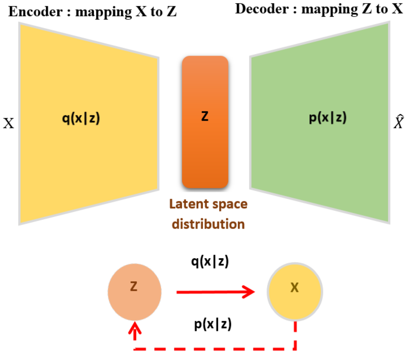
Figure 1. Basic schematic illustration of a variational autoencoder (VAE).
Applsci 10 08400 g001
Figure 2. Reconstruction loss and Kulback-Leibler (KL) divergence to train VAE.
Applsci 10 08400 g002
Figure 3. Schematic presentation of deep learning-based photovoltaic (PV) power forecasting.
Applsci 10 08400 g003
Figure 4. VAE-driven procedure.
Applsci 10 08400 g004
Figure 5. (a) distribution of solar PV power output from Parking Lot Canopy Array dataset. (b) Hourly distribution of solar PV power output from January to December 2018.
Applsci 10 08400 g005
Figure 6. Boxplots of PV power output during daytime hours: (a) Data Set 1 and (b) Data Set 2.
Applsci 10 08400 g006
Figure 7. Forecasting results from the eight models using the testing datasets: (a) Long Short-Term Memory Networks (LSTM), (b) gated recurrent unit (GRU), (c) recurrent neural network (RNN), (d) Bidirectional LSTM (BiLSTM), (e) Convolutional LSTM (ConvLSTM), (f) Restricted Boltzmann Machine (RBM), (g) stacked autoencoder (SAE) and (h) VAE.
Applsci 10 08400 g007
Figure 8. Scatter graphs of PV power forecasting and measurements using the eight models: (a) LSTM, (b) GRU, (c) RNN, (d) BiLSTM, (e) ConvLSTM, (f) RBM, (g) SAE, and (h) VAE.
Applsci 10 08400 g008
Figure 9. Scatter graphs of PV power forecasting and measurements using the eight models: (a) LSTM, (b) GRU, (c) RNN, (d) BiLSTM, (e) ConvLSTM, (f) RBM, (g) SAE, and (h) VAE.
Applsci 10 08400 g009
Figure 10. NRMSE by method based on the testing datasets from the two considered PV systems.
Applsci 10 08400 g010
Table 1. The considered benchmark deep learning methods.
ModelDescriptionKey Points
Applsci 10 08400 i001
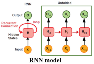
  • RNNs are able to include historical information in the forecasting process via their recurrent structure and memory units
  • Simple RNN do not have gates [39].
  • The RNNs are entirely trained in a supervised way.
+
Modeling time dependencies
-
Simple RNNs fail to catch the long-term evolution due to the vanishing gradient and exploding gradient [33].
Applsci 10 08400 i002
  • LSTM consists of three gates regulating the information flow called input, forge, and output gates [40].
  • Gate mechanism is used to store and memorize historical data features.
  • GRU use two gates, while LSTM is based on three gates.
+
LSTM showed good performance for learning long-term dependencies more easily than the conventional RNN
-
Its training is relatively longer than that of other RNN algorithms
-
The architecture of typical LSTM is very complex
Applsci 10 08400 i003
  • The major demarcation of GRU from LSTM is that only one unit is used to control both the forgetting factor and the decision to update the state unit [41].
  • GRU contains only two gates, the update, and the reset gates.
  • The GRU has been widely used in time-series, data sequence (e.g., speech and text processing), temporal features extraction, prediction, and forecasting.
+
The attractive features of the GRU model are the shorter training time compared to the LSTM and the fewer parameters that the GRU model possesses compared to the LSTM [41].
-
GRU models have problems such as slow convergence rate and low learning efficiency, resulting in too long training time and even under-fitting.
Applsci 10 08400 i004
  • Compared to the LSTM model that passes the input data through the network in one direction from past to future (forward), the BiLSTM processes the input also in the backward direction from the future to the past [42].
  • This architecture improves the learning of complex temporal dependencies through double processing.
+
Modeling time dependencies
+
Improved accuracy in state reconstruction is achieved by BiLSTM that merges the desirable features of both bidirectional RNN and LSTM [42].
-
Complex architecture
Applsci 10 08400 i005
  • The ConvLSTM is a special variant of the traditional LSTM, in which the fully-connected layer operators are replaced with convolutional operators [43].
  • LSTM with recurrent connection to deal with data sequences.
  • The convolutional layer can deal with 2D inputs like a sequence of images.
+
The ConvLSTM can process 2D input through convolutional transformations to learn the spatial features and then feed the LSTM module.
+
It has been used in modeling time dependencies, feature extraction, and spatiotemporal modeling
-
Complex architecture
Applsci 10 08400 i006
  • Autoencoders are neural networks that aim to create a compact representation of a given input x like images or any type of data [44].
  • The network learns how to compress the input features by keeping the most important information by minimizing the reconstruction error between the compressed input and the original input x [44].
  • Autoencoders are usually stacked to build a deep-stacked autoencoder.
+
Powerful compression capabilities
+
The SAEs are trained in an unsupervised way
+
They are applied for features extraction, data generation, dimensionality reduction, classification, prediction, and forecasting.
-
Suffers from the error vanishing and the overfitting
Applsci 10 08400 i007
  • RBMs are stochastic and generative neural networks [45] consisting of visible units and hidden units. There are no connections between visible-to-visible and hidden-to-hidden; however, visible and hidden units are fully connected.
  • Usually, RBMs are trained based on the contrastive divergence learning method.
  • Contrastive divergence uses Gibbs sampling to compute the intractable negative phase.
+
Simple architecture with two layers
+
Generative model,
+
Strong data distribution approximation.
+
Can be stacked to build a deep learning model like DBN or DBM.
-
Slow training due to Contrastive Divergence approach.
Table 2. Tuned parameters in the considered methods.
MethodsParameterValue
learning rate0.0005
RBMGibbs sampling (k)5
Training epochs500
Layers01
SEASLearning rate0.0005
Training epochs500
Layers04
VAELearning rate0.0005
Training epochs500
Layers05
RNNLearning rate0.0005
Training epochs500
GRULearning rate0.0005
Training epochs200
LSTMLearning rate0.0005
Training epochs200
BiLSTMLearning rate0.0005
Training epochs200
ConvLSTMLearning rate0.0005
Training epochs200
Table 3. Forecasting performance of the eight models based on testing data of the first dataset.
MethodR2RMSEMAEEV
LSTM0.9907.6723.9110.990
GRU0.9907.7684.0220.990
RNN0.9917.5394.0720.991
BiLSTM0.9907.7223.9100.990
ConvLSTM0.83231.84216.3380.832
RBM0.92920.6728.9100.929
SAE0.93220.3018.3000.932
SVM0.97114.17412.8890.972
LG0.96515.459.9420.966
VAE0.9955.4713.2320.995
Table 4. Forecasting performance of the eight methods using the test set of the second dataset.
MethodR2RMSEMAEEV
LSTM0.992246.781107.7990.992
GRU0.991250.004117.6220.992
RNN0.992241.170125.9600.992
BiLSTM0.991259.884117.5790.991
ConvLSTM0.6921500.070846.7500.692
RBM0.977407.238170.5680.977
SAE0.983349.066124.7720.983
SVM0.924770.996699.8370.954
LG0.899886.665837.7210.926
VAE0.995199.64599.8380.995
Table 5. Validation metrics for multistep-step-ahead forecasts.
AlgerianPVSystem ParkingLotCanopyArray
ModelStepsMinutesRMSEMAER2EVRMSEMAER2EV
BiLSTM2301591.6391303.280.6750.87618.30910.0110.9510.953
CNN2301007.54613.3440.870.88824.10516.5340.9150.916
ConvLSTM2D230359.128262.5260.9830.99117.317.7860.9560.956
GRU230910.589770.9070.8940.93617.4547.8970.9550.955
LSTM230376.359285.3240.9820.98217.477.9140.9550.955
RBM230390.581213.1740.980.9817.5647.8470.9550.955
RNN2301448.0631170.2790.7310.86818.1018.4740.9520.953
SAE230477.986255.7390.9710.97417.7248.7830.9540.955
VAE230303.091117.7010.9880.98817.317.5660.9560.956
BiLSTM345374.303186.5760.9820.98221.85512.0280.930.93
CNN3451166.323749.8630.8260.8426.13518.6170.90.9
ConvLSTM2D345370.848260.9220.9820.98621.31510.3970.9330.934
GRU345395.163225.1540.980.9821.7811.5960.930.932
LSTM345367.048194.6910.9830.98321.4859.7070.9320.932
RBM345579.104341.1510.9570.95821.7610.4340.9310.931
RNN345428.615284.60.9760.97722.45811.990.9260.93
SAE345521.723255.6860.9650.96921.82310.3350.930.93
VAE345344.468164.6350.9850.98521.4619.8780.9320.932
BiLSTM460432.448229.340.9760.97723.68713.1310.9180.92
CNN460949.999567.3580.8840.89727.02217.5020.8930.9
ConvLSTM2D460462.93360.6180.9720.97823.17412.1130.9210.921
GRU460538.857381.6860.9630.96523.25211.6810.9210.921
LSTM460533.916355.0420.9630.96623.29811.9120.920.921
RBM460614.722379.4060.9510.95123.32111.6050.920.92
RNN460476.67297.1960.9710.97124.15213.2080.9140.918
SAE460554.917274.5360.960.96123.60411.7680.9180.918
VAE460420.029193.1570.9770.97823.13411.6640.9210.921
Publisher’s Note: MDPI stays neutral with regard to jurisdictional claims in published maps and institutional affiliations.