A Cell Counting Framework Based on Random Forest and Density Map

Abstract
1. Introduction
- A dilated feature extraction was proposed to reduce the spatial redundancy and mitigate computation overhead.
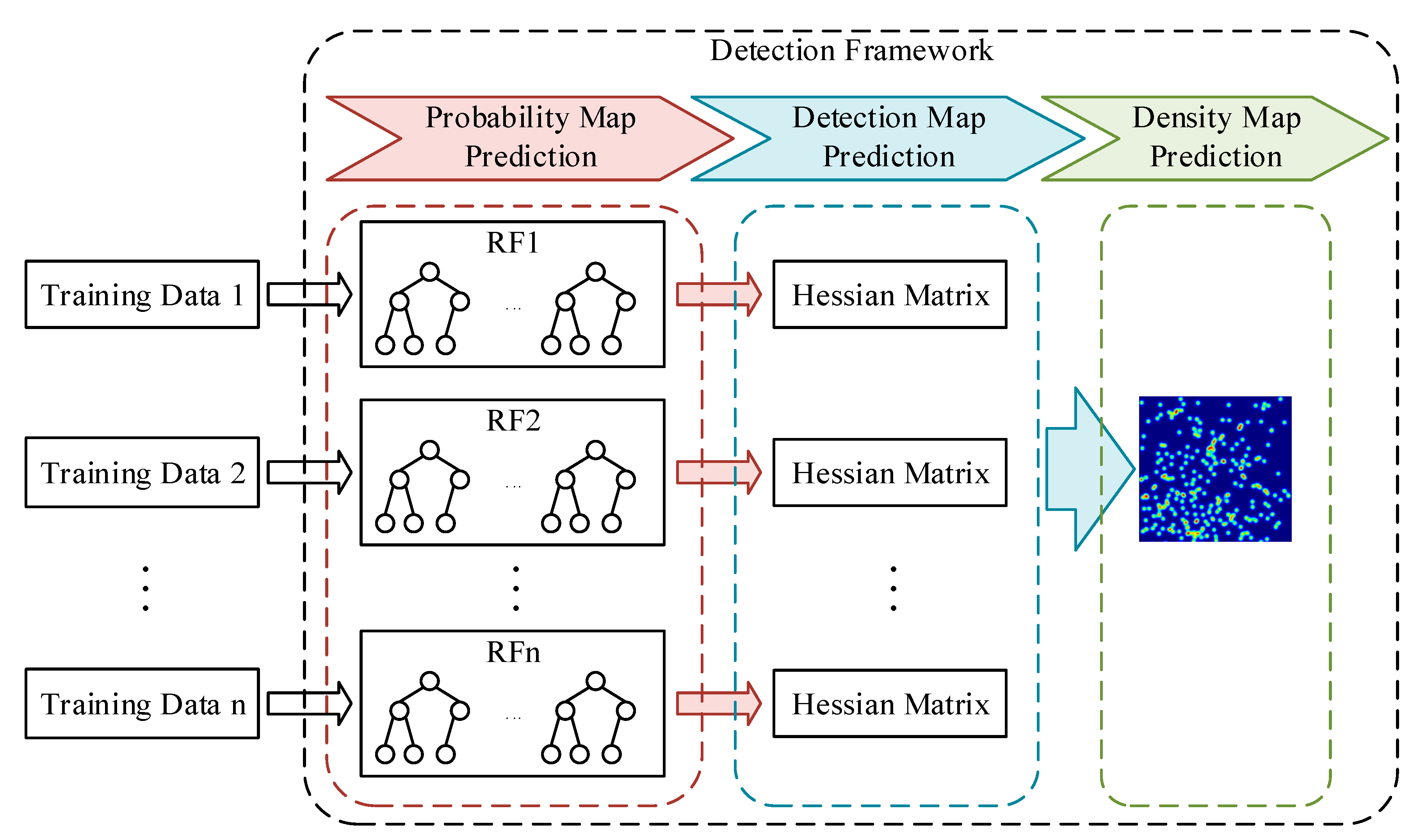
- We proposed a CCF that contains multiple RFs. Different RFs will generate different probability maps. Taking advantage of the proposed probability map, we suggested to locating the cells by the eigenvalue of the Hessian matrix. After combining all the detection results, the overall count error was decreased.
- We validated the proposed model on three different kinds of cell datasets and the results prove that our model is competitive to the CNN-based models and even better. In addition, the comparison results between the proposed CCF and the individual RF prove that the CCF has lower bias and variance than the individual RF.
2. Related Work
3. Method
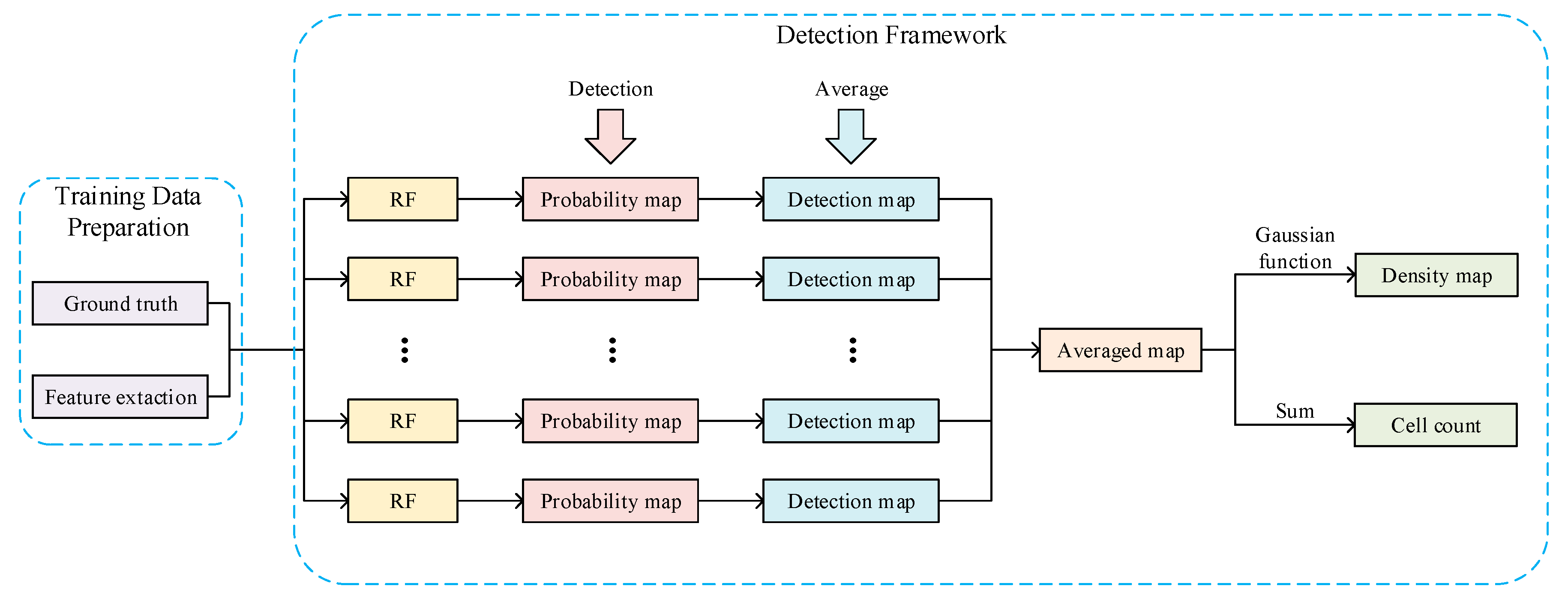
3.1. Training Data Preparation
3.1.1. Ground Truth Generation
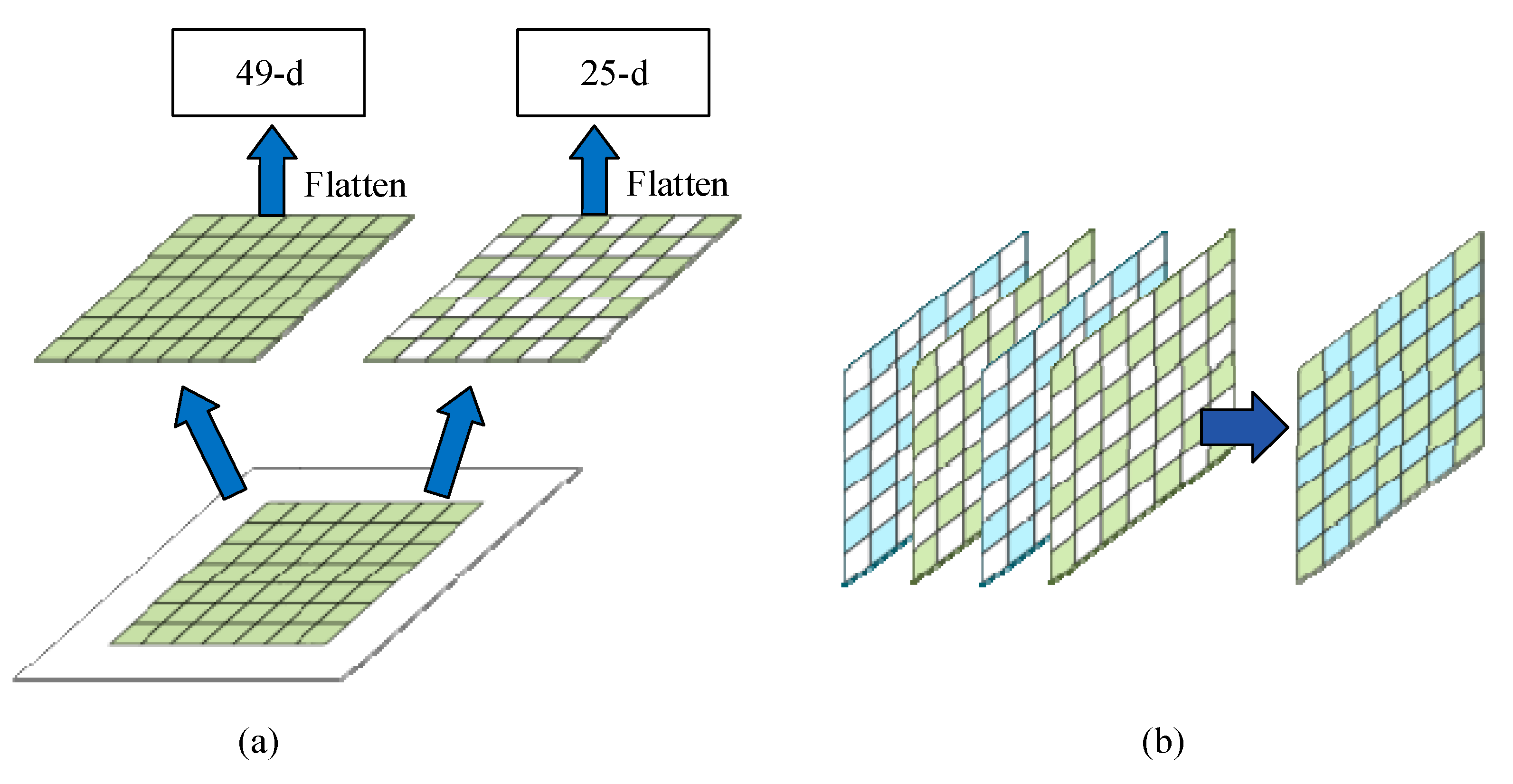
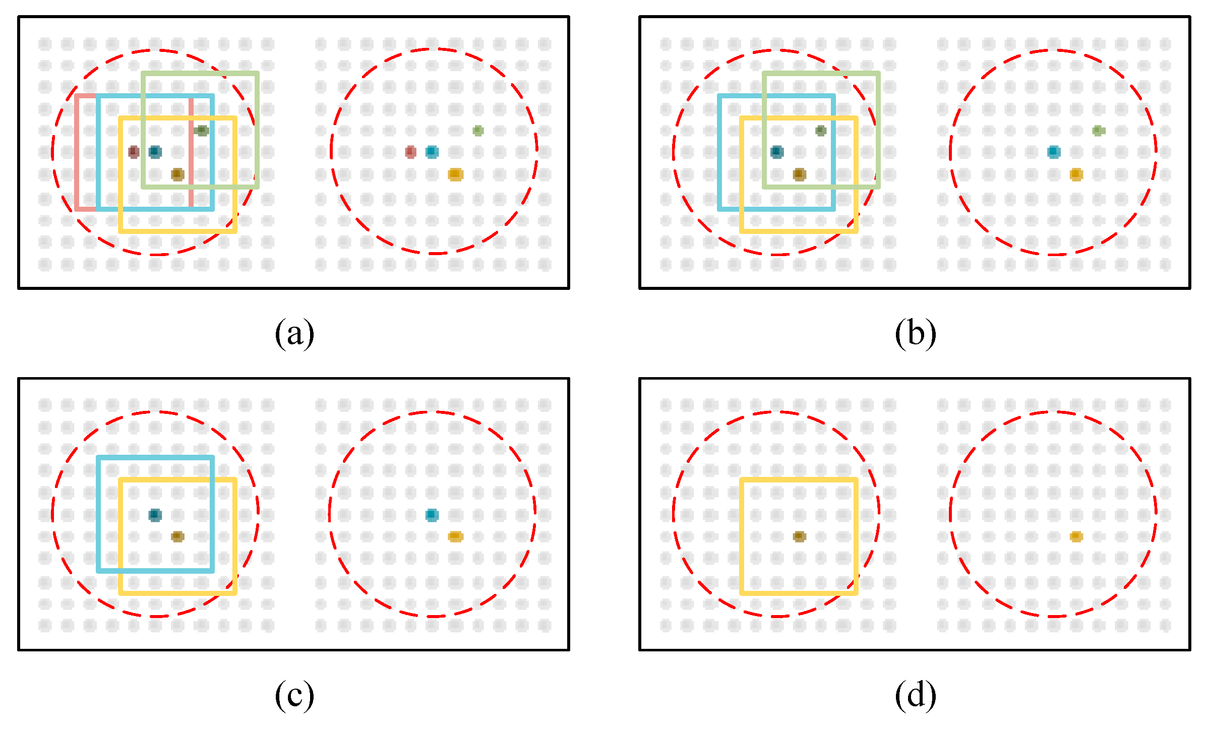
3.1.2. Dilated Feature Extraction
3.2. Detection Framework
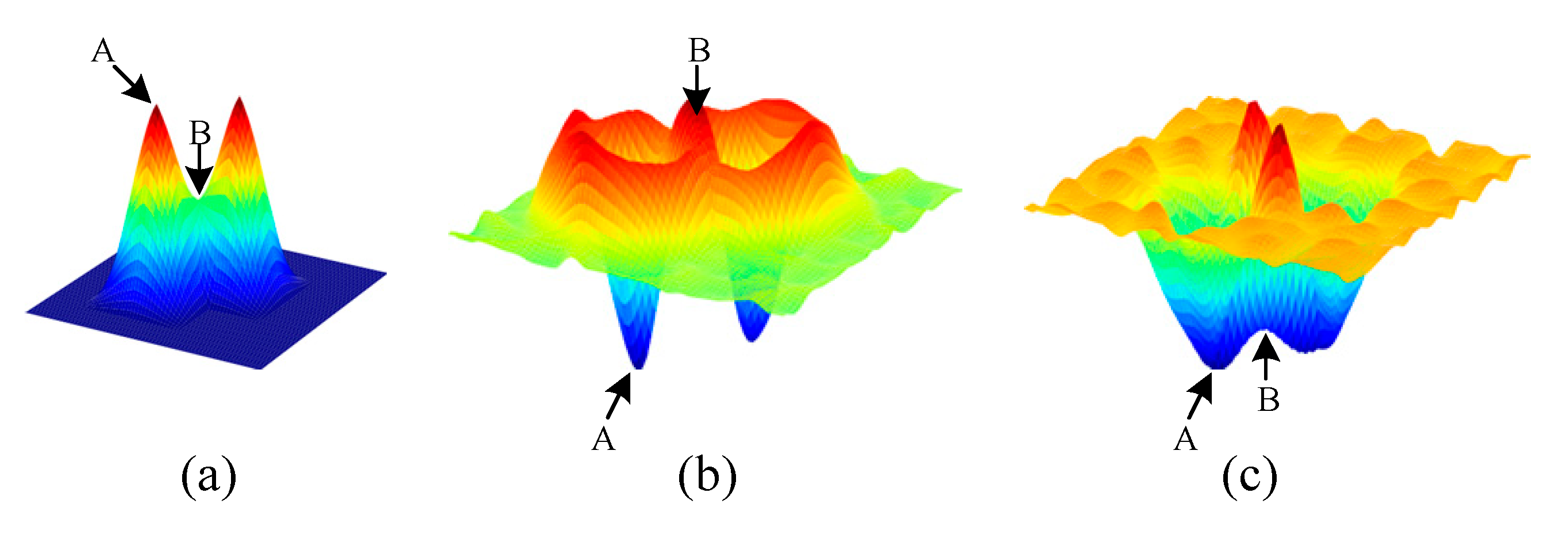
3.2.1. Probability Map Prediction
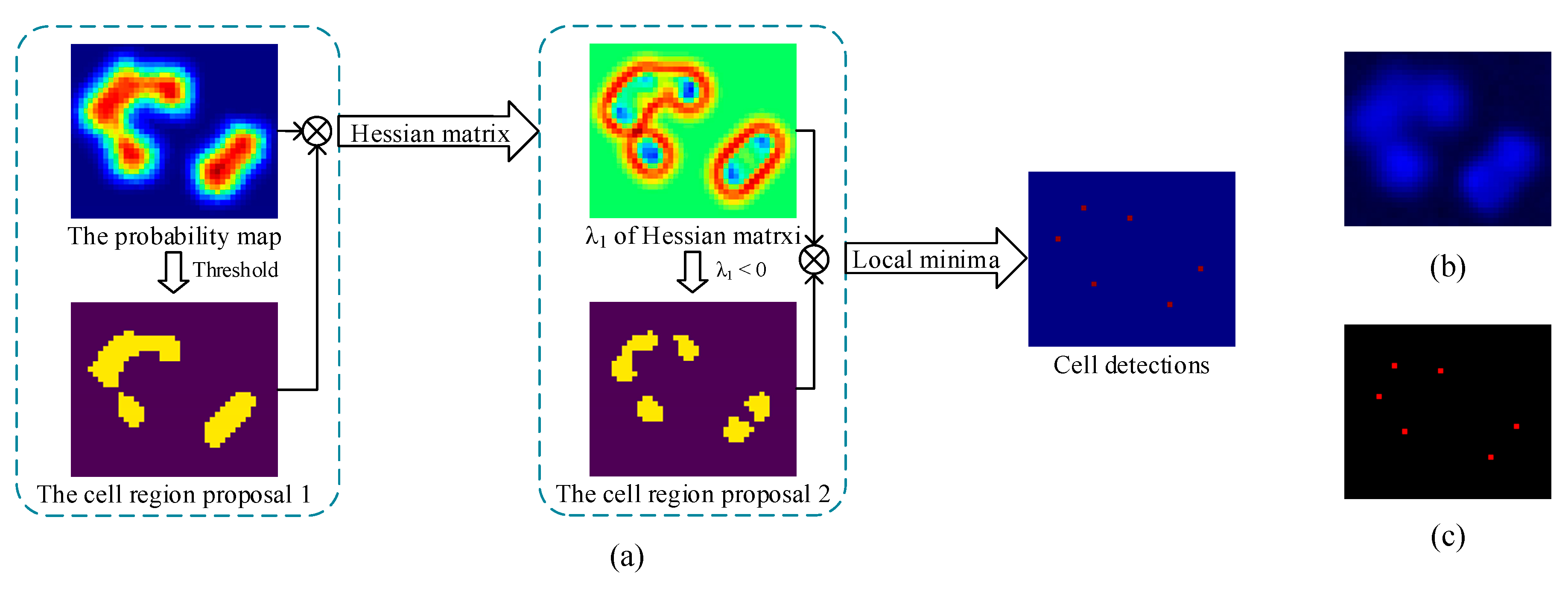
3.2.2. Detection Map Generation
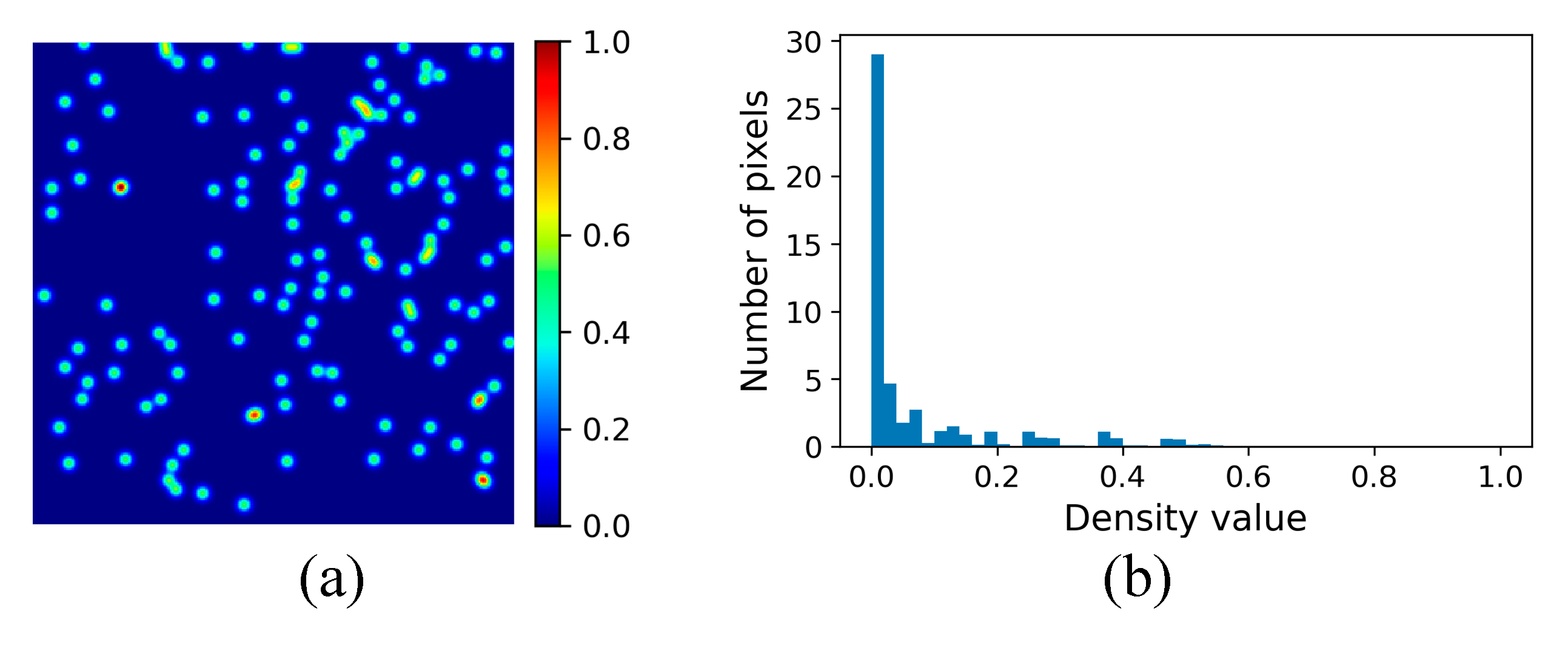
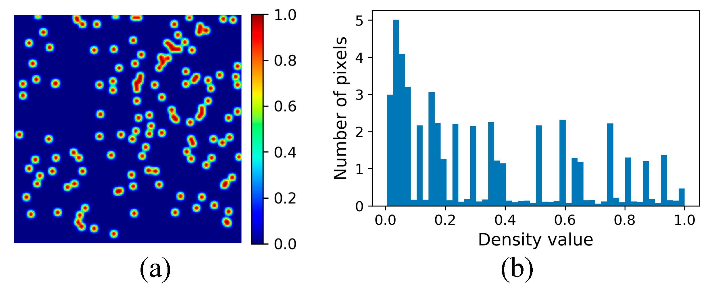
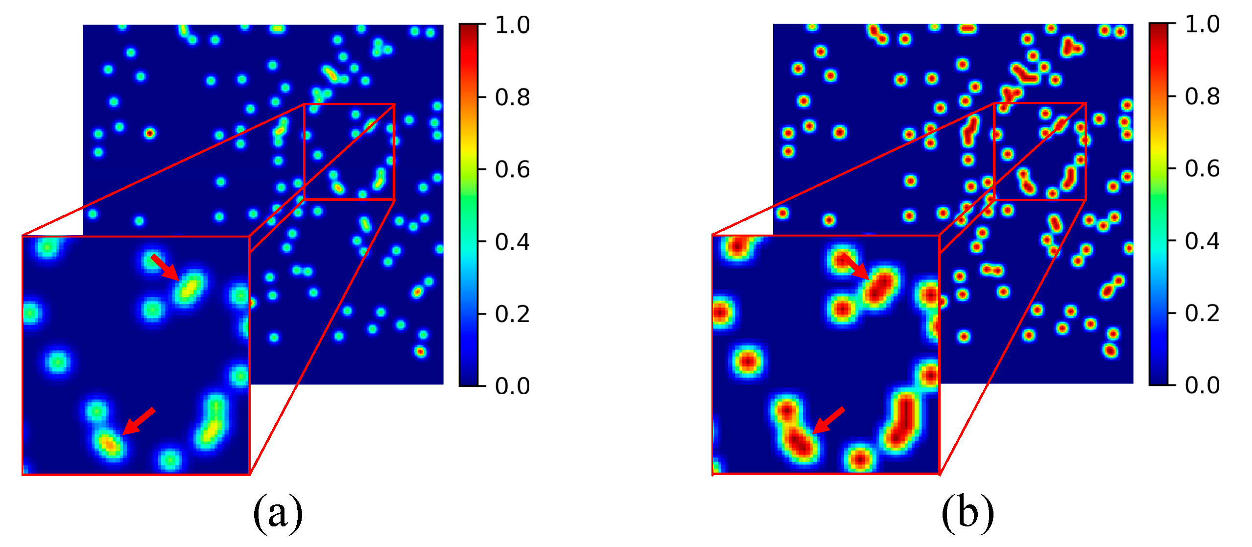
3.2.3. Density Map Generation
4. Experiments and Results
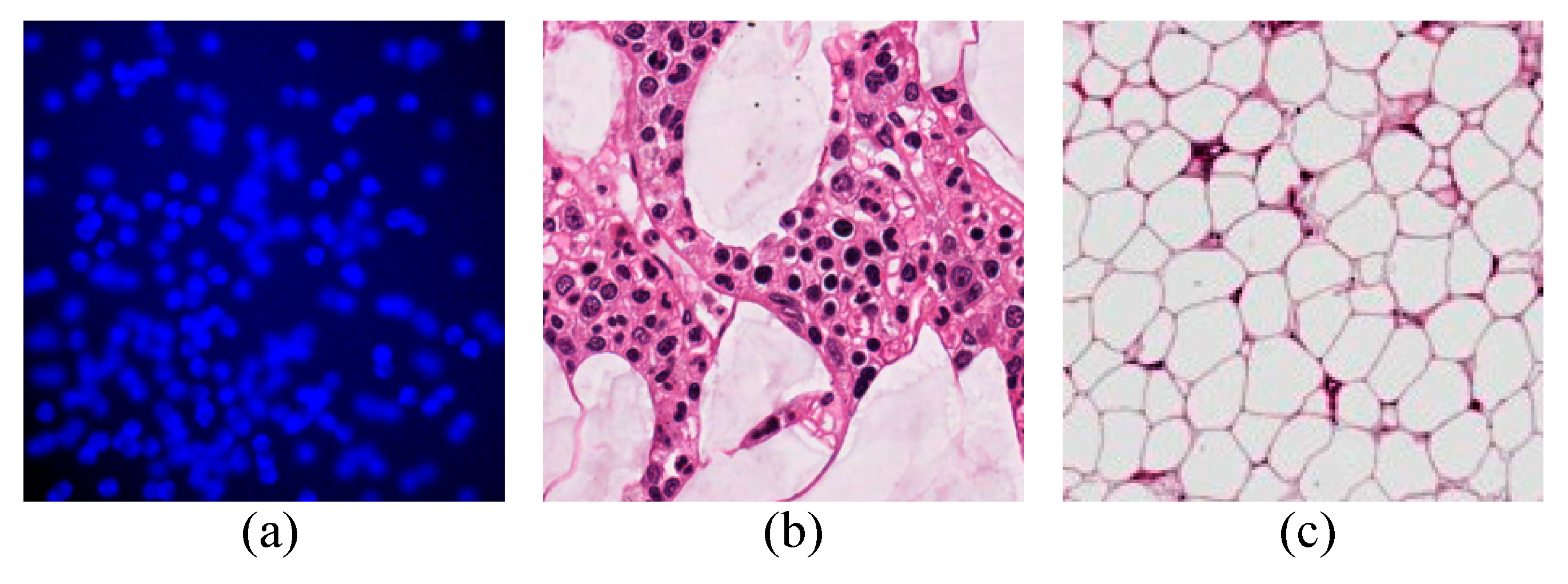
4.1. Datasets
4.2. Evaluation Metric
4.3. Results and Discussion
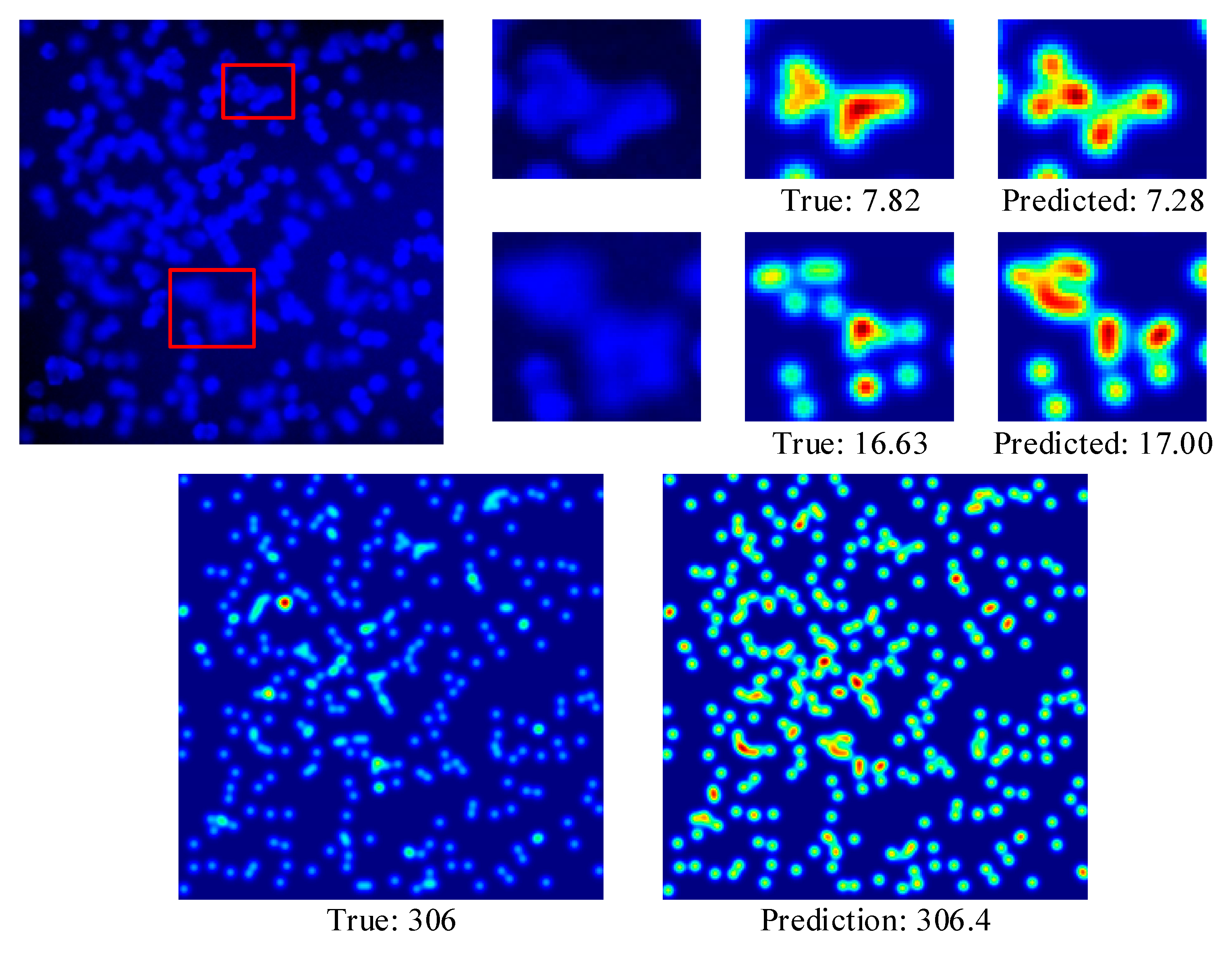
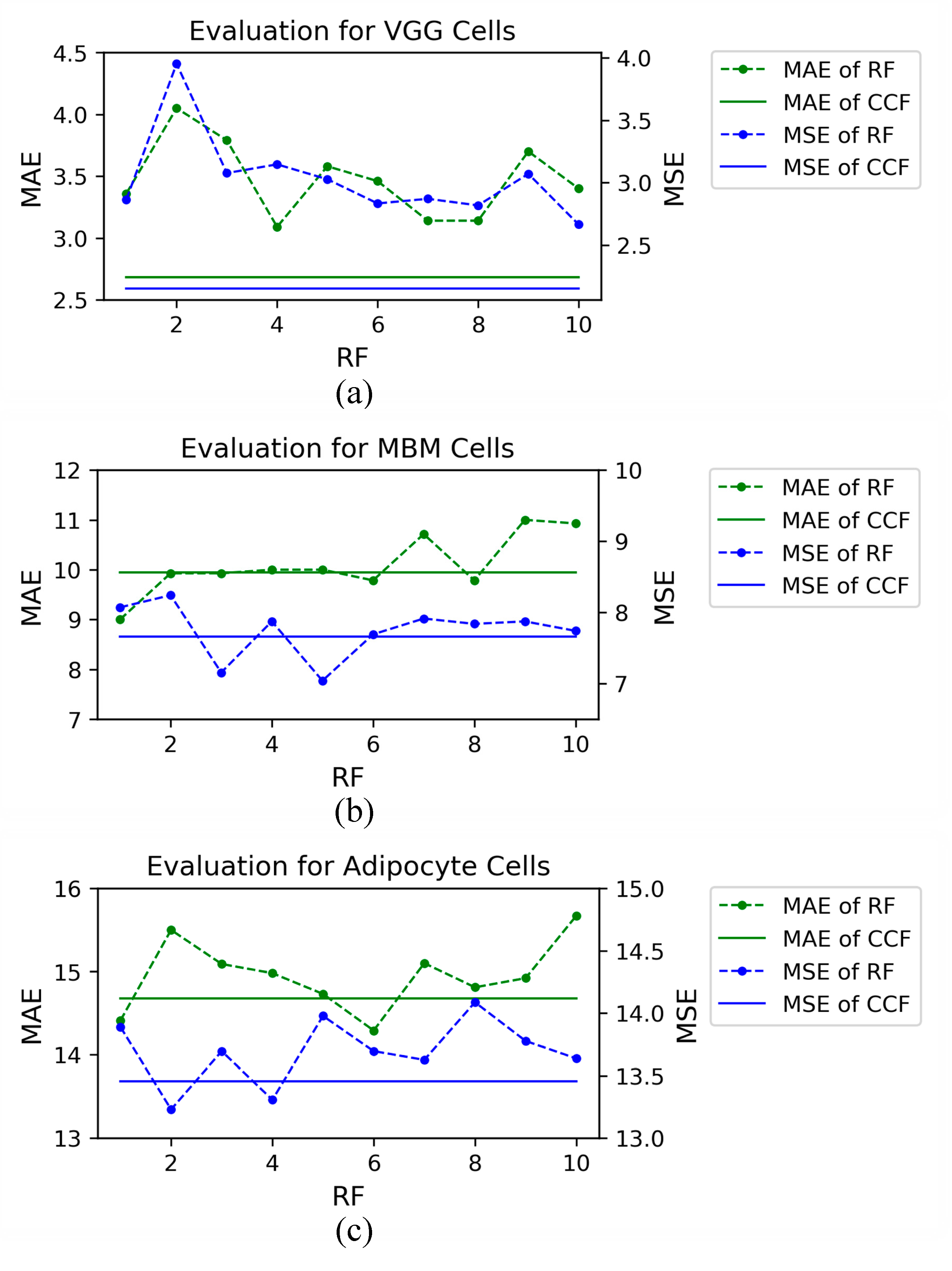
4.3.1. VGG Cells
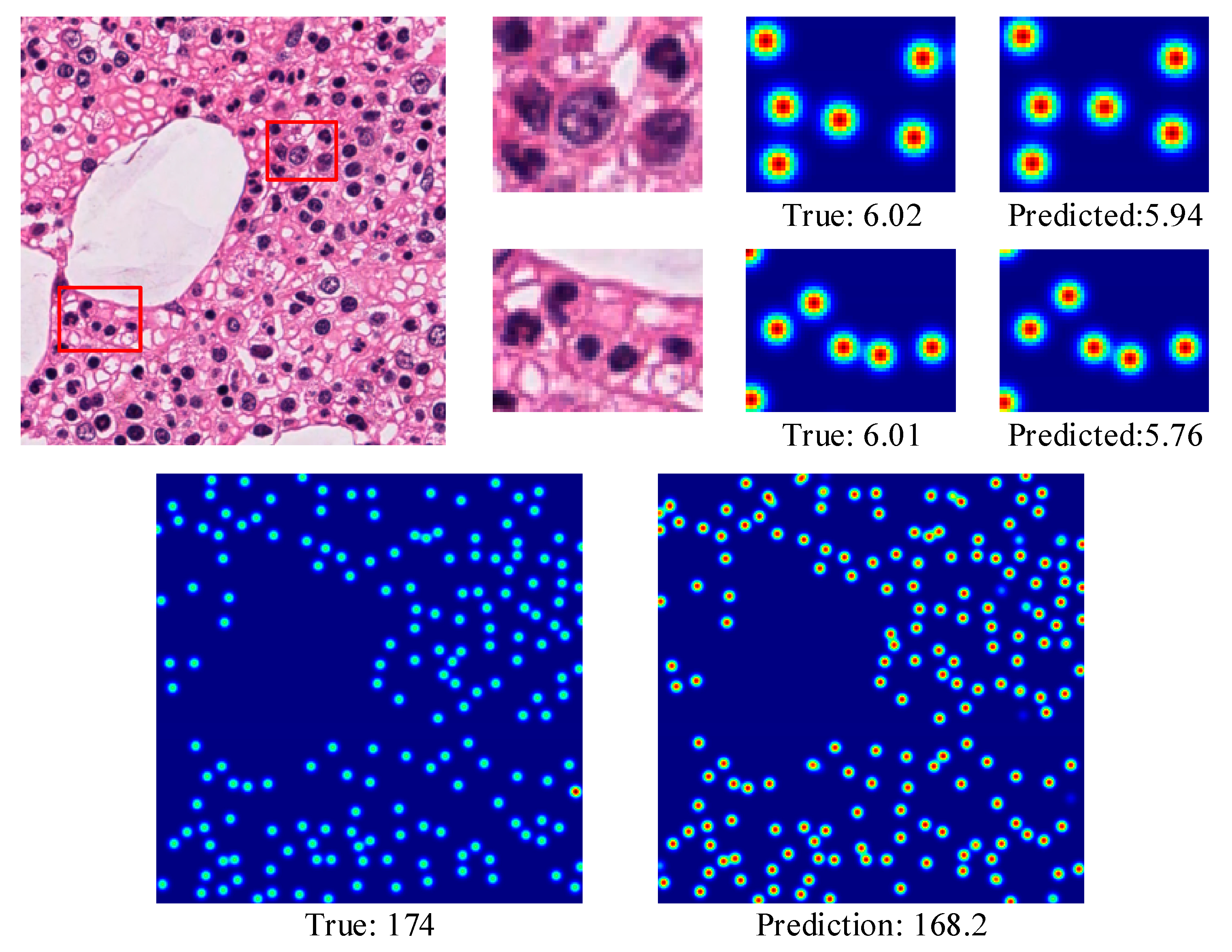
4.3.2. MBM Cells
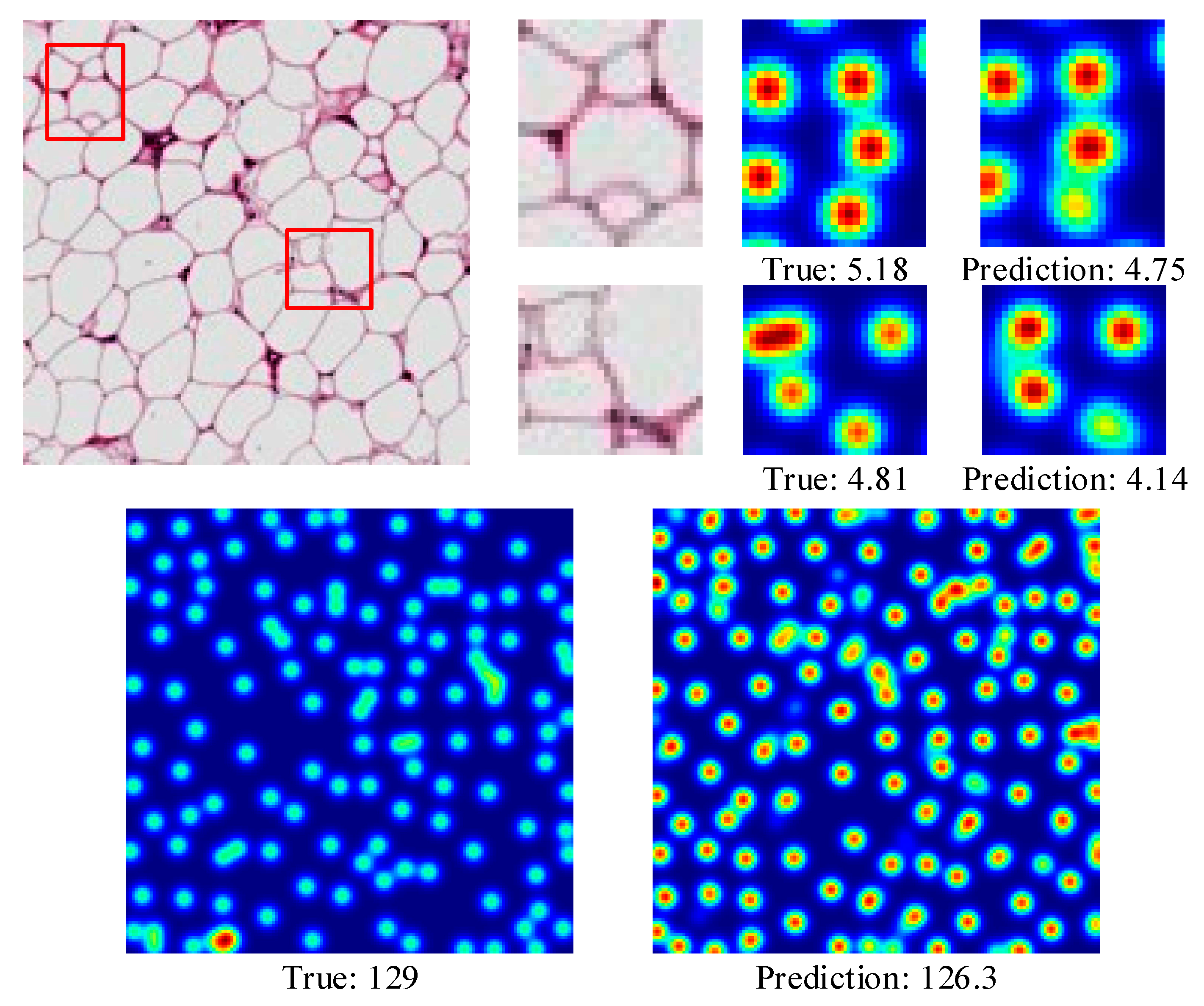
4.3.3. Adipocyte Cells
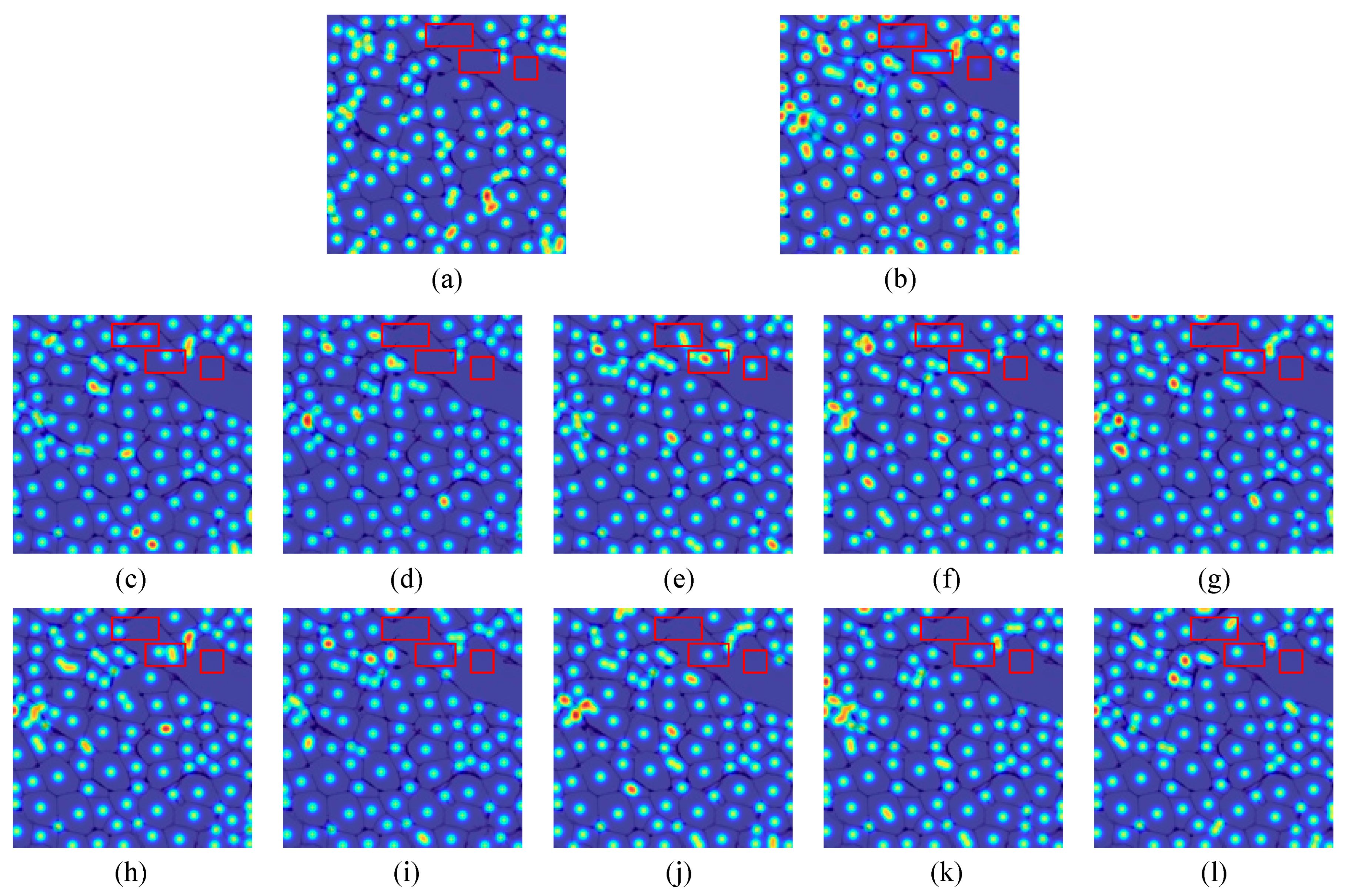
4.3.4. The Effectiveness of CCF
5. Conclusions
Author Contributions
Funding
Conflicts of Interest
References
- Lempitsky, V.; Zisserman, A. Learning to count objects in images. In Proceedings of the Advances in Neural Information Processing Systems, Vancouver, BC, Canada, 6–9 December 2010; pp. 1324–1332. [Google Scholar]
- Fiaschi, L.; Köthe, U.; Nair, R.; Hamprecht, F.A. Learning to count with regression forest and structured labels. In Proceedings of the 21st International Conference on Pattern Recognition (ICPR2012), Tsukuba, Japan, 11–15 November 2012; pp. 2685–2688. [Google Scholar]
- Sommer, C.; Straehle, C.; Koethe, U.; Hamprecht, F.A. Ilastik: Interactive learning and segmentation toolkit. In Proceedings of the 2011 IEEE International Symposium on Biomedical Imaging: From Nano to Macro, Chicago, IL, USA, 30 March–2 April 2011; pp. 230–233. [Google Scholar]
- Magana-Tellez, O.; Vrigkas, M.; Nikou, C.; Kakadiaris, I.A. SPICE: Superpixel Classification for Cell Detection and Counting. In Proceedings of the 13th International Conference on Computer Vision Theory and Applications, Funchal, Madeira, Portugal, 27–29 January 2018; pp. 485–490. [Google Scholar]
- Xie, W.; Noble, J.A.; Zisserman, A. Microscopy cell counting and detection with fully convolutional regression networks. Comput. Methods Biomech. Biomed. Eng. Imaging Vis. 2018, 6, 283–292. [Google Scholar] [CrossRef]
- Paul Cohen, J.; Boucher, G.; Glastonbury, C.A.; Lo, H.Z.; Bengio, Y. Count-ception: Counting by fully convolutional redundant counting. In Proceedings of the 2017 IEEE International Conference on Computer Vision Workshops (ICCVW), Venice, Italy, 22–29 October 2017; pp. 18–26. [Google Scholar]
- Kainz, P.; Urschler, M.; Schulter, S.; Wohlhart, P.; Lepetit, V. You should use regression to detect cells. In Proceedings of the Medical Image Computing and Computer-Assisted Intervention—MICCAI 2015, Munich, Germany, 5–9 October 2015; pp. 276–283. [Google Scholar]
- Pan, X.; Yang, D.; Li, L.; Liu, Z.; Yang, H.; Cao, Z.; He, Y.; Ma, Z.; Chen, Y. Cell detection in pathology and microscopy images with multi-scale fully convolutional neural networks. World Wide Web 2018, 21, 1721–1743. [Google Scholar] [CrossRef]
- Liang, H.; Naik, A.; Williams, C.L.; Kapur, J.; Weller, D.S. Enhanced center coding for cell detection with convolutional neural networks. arXiv 2019, arXiv:1904.08864. [Google Scholar]
- Zhu, R.; Sui, D.; Qin, H.; Hao, A. An extended type cell detection and counting method based on FCN. In Proceedings of the 2017 IEEE 17th International Conference on Bioinformatics and Bioengineering (BIBE), Washington, DC, USA, 23–25 October 2017; pp. 51–56. [Google Scholar]
- Ronneberger, O.; Fischer, P.; Brox, T. U-net: Convolutional networks for biomedical image segmentation. In Proceedings of the Medical Image Computing and Computer-Assisted Intervention—MICCAI 2015, Munich, Germany, 5–9 October 2015; pp. 234–241. [Google Scholar]
- He, K.; Zhang, X.; Ren, S.; Sun, J. Deep residual learning for image recognition. In Proceedings of the 2016 IEEE Conference on Computer Vision and Pattern Recognition (CVPR), Las Vegas, NV, USA, 27–30 June 2016; pp. 770–778. [Google Scholar]
- Yu, F.; Koltun, V. Multi-scale context aggregation by dilated convolutions. arXiv 2015, arXiv:1511.07122. [Google Scholar]
- Rad, R.M.; Saeedi, P.; Au, J.; Havelock, J. Blastomere cell counting and centroid localization in microscopic images of human embryo. In Proceedings of the 2018 IEEE 20th International Workshop on Multimedia Signal Processing (MMSP), Vancouver, BC, Canada, 29–31 August 2018; pp. 1–6. [Google Scholar]
- Xie, Y.; Xing, F.; Kong, X.; Su, H.; Yang, L. Beyond classification: Structured regression for robust cell detection using convolutional neural network. In Proceedings of the Medical Image Computing and Computer-Assisted Intervention—MICCAI 2015, Munich, Germany, 5–9 October 2015; pp. 358–365. [Google Scholar]
- Ma, Z.; Yu, L.; Chan, A.B. Small instance detection by integer programming on object density maps. In Proceedings of the 2015 IEEE Conference on Computer Vision and Pattern Recognition (CVPR), Boston, MA, USA, 7–12 June 2015; pp. 3689–3697. [Google Scholar]
- Akram, S.U.; Kannala, J.; Eklund, L.; Heikkilä, J. Cell segmentation proposal network for microscopy image analysis. In Proceedings of the Deep Learning and Data Labeling for Medical Applications, Athens, Greece, 21 October 2016; pp. 21–29. [Google Scholar]
- Xue, Y.; Ray, N. Cell Detection in microscopy images with deep convolutional neural network and compressed sensing. arXiv 2017, arXiv:1708.03307. [Google Scholar]
- Wang, X.; Girshick, R.; Gupta, A.; He, K. Non-local neural networks. In Proceedings of the 2018 IEEE/CVF Conference on Computer Vision and Pattern Recognition, Salt Lake City, UT, USA, 18–23 June 2018; pp. 7794–7803. [Google Scholar]
- Zhang, H.; Goodfellow, I.; Metaxas, D.; Odena, A. Self-attention generative adversarial networks. In Proceedings of the 36th International Conference on Machine Learning, Long Beach, CA, USA, 9–15 June 2019; pp. 7354–7363. [Google Scholar]
- Guo, Y.; Stein, J.; Wu, G.; Krishnamurthy, A. SAU-Net: A Universal Deep Network for Cell Counting. In Proceedings of the 10th ACM International Conference on Bioinformatics, Computational Biology and Health Informatics, Niagara Falls, NY, USA, 7–10 September 2019; pp. 299–306. [Google Scholar]
- Maitra, M.; Gupta, R.K.; Mukherjee, M. Detection and counting of red blood cells in blood cell images using Hough transform. Int. J. Comput. Appl. 2012, 53, 13–17. [Google Scholar] [CrossRef]
- Faustino, G.M.; Gattass, M.; Rehen, S.; de Lucena, C.J. Automatic embryonic stem cells detection and counting method in fluorescence microscopy images. In Proceedings of the 2009 IEEE International Symposium on Biomedical Imaging: From Nano to Macro, Boston, MA, USA, 28 June–1 July 2009; pp. 799–802. [Google Scholar]
- Kothari, S.; Chaudry, Q.; Wang, M.D. Automated cell counting and cluster segmentation using concavity detection and ellipse fitting techniques. In Proceedings of the 2009 IEEE International Symposium on Biomedical Imaging: From Nano to Macro, Boston, MA, USA, 28 June–1 July 2009; pp. 795–798. [Google Scholar]
- Zhang, C.; Sun, C.; Su, R.; Pham, T.D. Segmentation of clustered nuclei based on curvature weighting. In Proceedings of the 27th Conference on Image and Vision Computing, Dunedin, New Zealand, 26–28 November 2012; pp. 49–54. [Google Scholar]
- Jung, C.; Kim, C.; Chae, S.W.; Oh, S. Unsupervised segmentation of overlapped nuclei using Bayesian classification. IEEE Trans. Biomed. Eng. 2010, 57, 2825–2832. [Google Scholar] [CrossRef] [PubMed]
- Chen, L.-C.; Papandreou, G.; Kokkinos, I.; Murphy, K.; Yuille, A.L. Deeplab: Semantic image segmentation with deep convolutional nets, atrous convolution, and fully connected crfs. IEEE Trans. Pattern Anal. Mach. Intell. 2017, 40, 834–848. [Google Scholar] [CrossRef] [PubMed]
- Lonsdale, J.; Thomas, J.; Salvatore, M.; Phillips, R.; Lo, E.; Shad, S.; Hasz, R.; Walters, G.; Garcia, F.; Young, N. The genotype-tissue expression (GTEx) project. Nat. Genet. 2013, 45, 580–585. [Google Scholar] [CrossRef] [PubMed]
- Rad, R.M.; Saeedi, P.; Au, J.; Havelock, J. Cell-net: Embryonic cell counting and centroid localization via residual incremental atrous pyramid and progressive upsampling convolution. IEEE Access 2019, 7, 81945–81955. [Google Scholar]
- Arteta, C.; Lempitsky, V.; Noble, J.A.; Zisserman, A. Interactive object counting. In Proceedings of the Computer Vision—ECCV 2014, Zurich, Switzerland, 6–12 September 2014; pp. 504–518. [Google Scholar]
- Marsden, M.; McGuinness, K.; Little, S.; Keogh, C.E.; O’Connor, N.E. People, penguins and petri dishes: Adapting object counting models to new visual domains and object types without forgetting. In Proceedings of the 2018 IEEE/CVF Conference on Computer Vision and Pattern Recognition, Salt Lake City, UT, USA, 18–23 June 2018; pp. 8070–8079. [Google Scholar]
- Carpenter, A.E.; Jones, T.R.; Lamprecht, M.R.; Clarke, C.; Kang, I.H.; Friman, O.; Guertin, D.A.; Chang, J.H.; Lindquist, R.A.; Moffat, J. CellProfiler: Image analysis software for identifying and quantifying cell phenotypes. Genome Biol. 2006, 7, R100. [Google Scholar] [CrossRef] [PubMed]
- Galarraga, M.; Campión, J.; Muñoz-Barrutia, A.; Boqué, N.; Moreno, H.; Martínez, J.A.; Milagro, F.; Ortiz-de-Solórzano, C. Adiposoft: Automated software for the analysis of white adipose tissue cellularity in histological sections. J. Lipid Res. 2012, 53, 2791–2796. [Google Scholar] [CrossRef] [PubMed]


| Dataset | Resolution | Average | ||
|---|---|---|---|---|
| VGG cells [1] | 100 | 100 | ||
| MBM cells [6,7] | 30 | 14 | ||
| Adipocyte cells [28] | 100 | 100 |
| Method | ||||
|---|---|---|---|---|
| Lempitsky et al. [1] | 1 | |||
| Fiaschi et al. [2] | ||||
| Arteta et al. [30] | ||||
| FCRN-A [5] | 2 | |||
| SAU-Net [21] | 2 | |||
| Count-ception [6] | ||||
| CCF |
| Method | |||
|---|---|---|---|
| FCRN-A [5] | |||
| Count-ception [10] | |||
| Marsden et al. [31] | |||
| Cell-Net [29] | |||
| CCF |
| Method | |||
|---|---|---|---|
| CellProfiler [32] | ---------------------------------------- | ||
| Adiposoft [33] | ---------------------------------------- | ||
| Count-ception [6] | |||
| SAU-Net [21] | |||
| CCF | |||
Publisher’s Note: MDPI stays neutral with regard to jurisdictional claims in published maps and institutional affiliations. |
© 2020 by the authors. Licensee MDPI, Basel, Switzerland. This article is an open access article distributed under the terms and conditions of the Creative Commons Attribution (CC BY) license (http://creativecommons.org/licenses/by/4.0/).
Share and Cite
Jiang, N.; Yu, F. A Cell Counting Framework Based on Random Forest and Density Map. Appl. Sci. 2020, 10, 8346. https://doi.org/10.3390/app10238346
Jiang N, Yu F. A Cell Counting Framework Based on Random Forest and Density Map. Applied Sciences. 2020; 10(23):8346. https://doi.org/10.3390/app10238346
Chicago/Turabian StyleJiang, Ni, and Feihong Yu. 2020. "A Cell Counting Framework Based on Random Forest and Density Map" Applied Sciences 10, no. 23: 8346. https://doi.org/10.3390/app10238346
APA StyleJiang, N., & Yu, F. (2020). A Cell Counting Framework Based on Random Forest and Density Map. Applied Sciences, 10(23), 8346. https://doi.org/10.3390/app10238346