Deep Learning-Based Pixel-Wise Lesion Segmentation on Oral Squamous Cell Carcinoma Images

 ,
,  ,
,  ,
, 
Abstract
1. Introduction
- WSI are extremely large images, having a memory size of two gigabytes on average [6].
- There are a few surgical pathology units that are fully digitalized and that can store a large amount of digitalized slides, although their number is increasing exponentially [7].
- There is a small number of available image datasets and most of them are not annotated [8].
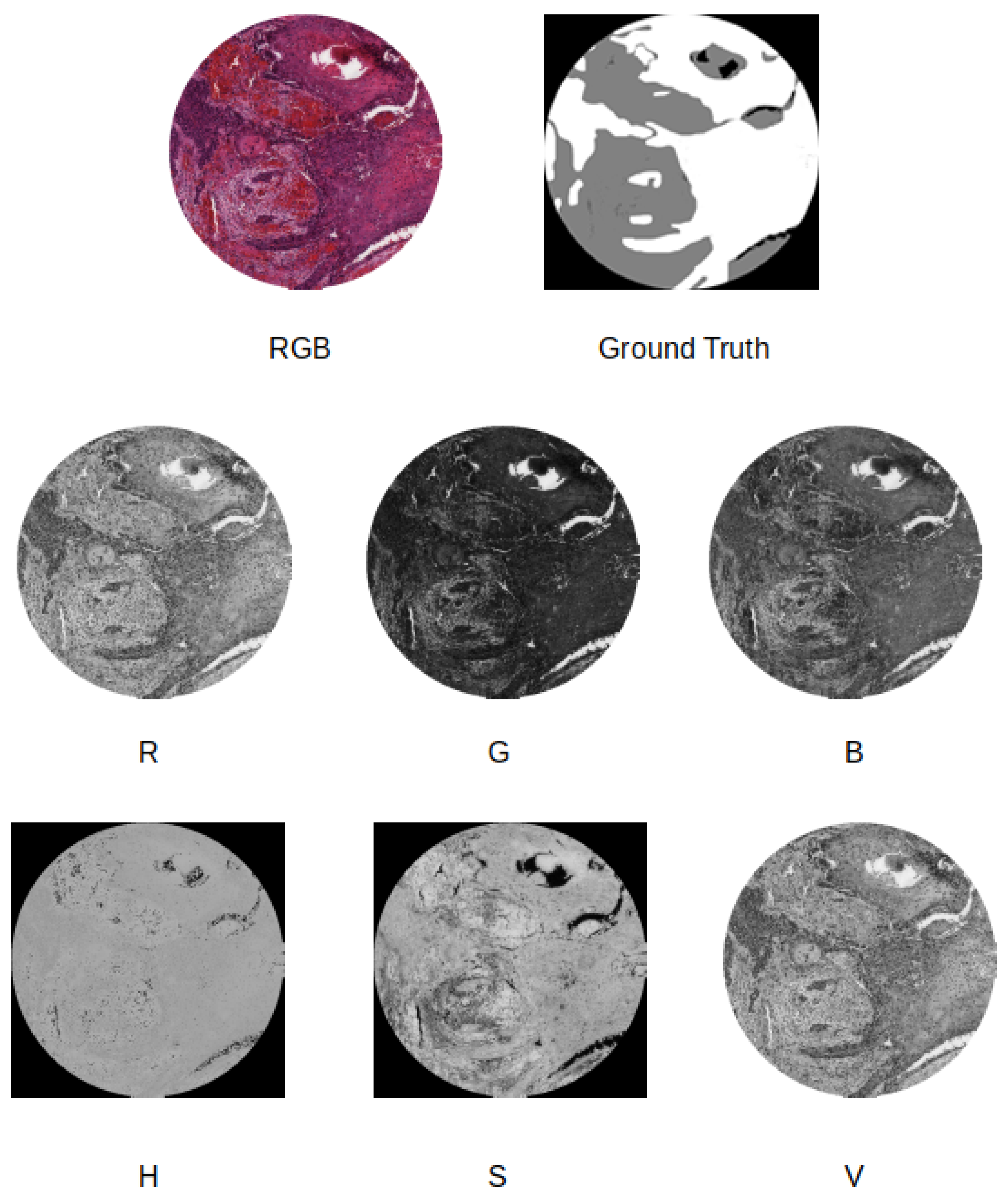
- We compare four different supervised pixel-wise segmentation methods for detecting carcinoma areas in WSI using quantitative metrics. Different input formats, including separating the color channels in the RGB and Hue, Saturation, and Value (HSV) models, are taken into account in the experiments.
- We use two different image datasets, one for training and another one for testing. This allows us to understand the real generalization capabilities of the considered SSNs.
- We created a publicly available dataset, called Oral Cancer Annotated (ORCA) dataset, containing annotated data from the Cancer Genome Atlas (TCGA) dataset, which can be used by other researchers for testing their approaches.
2. Related Work
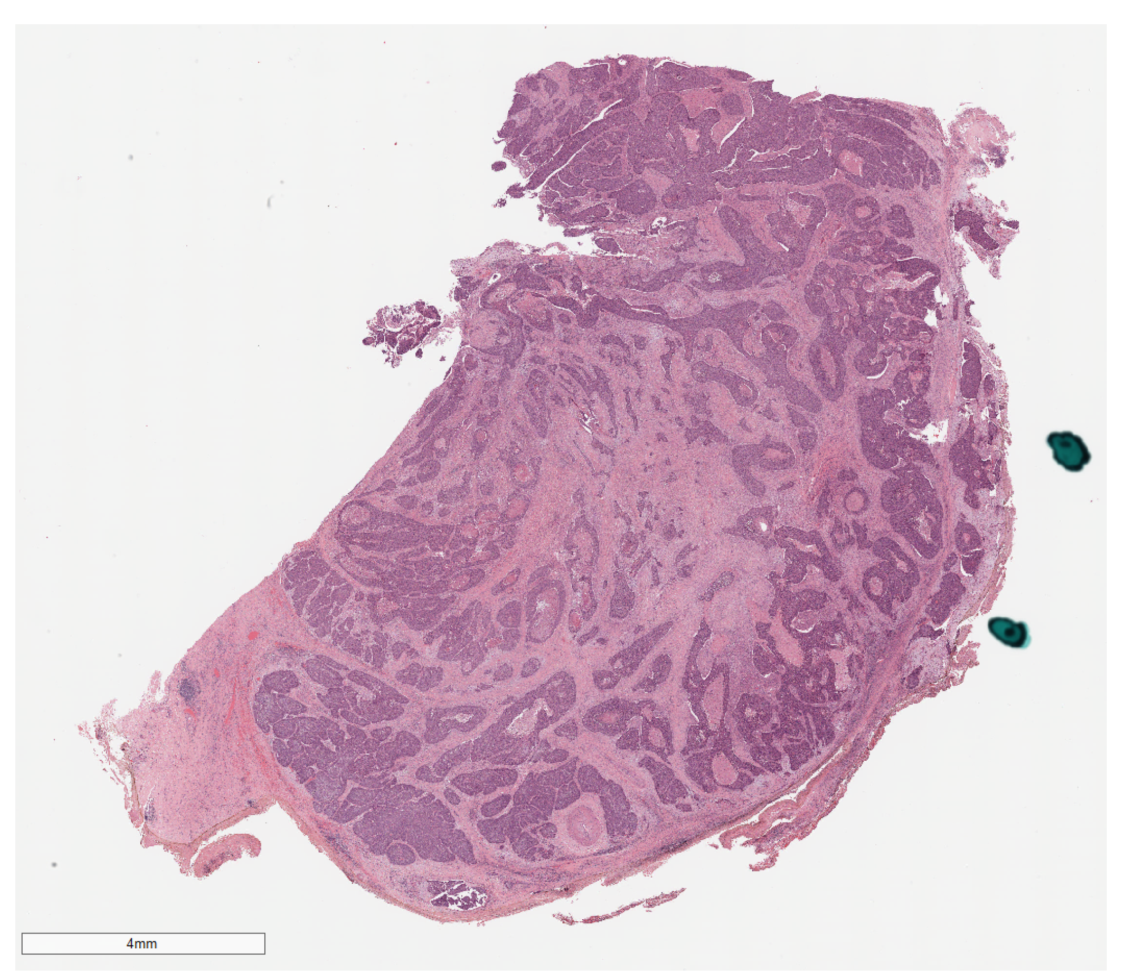
Datasets
3. Methods
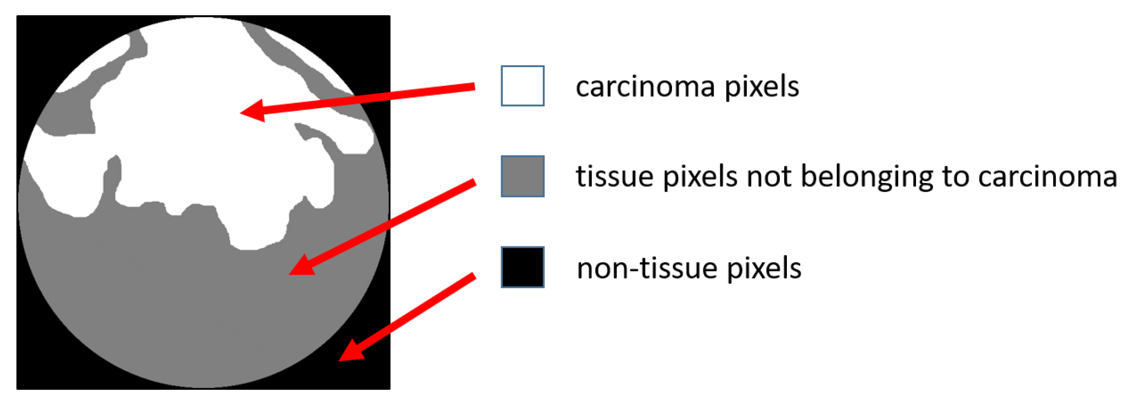
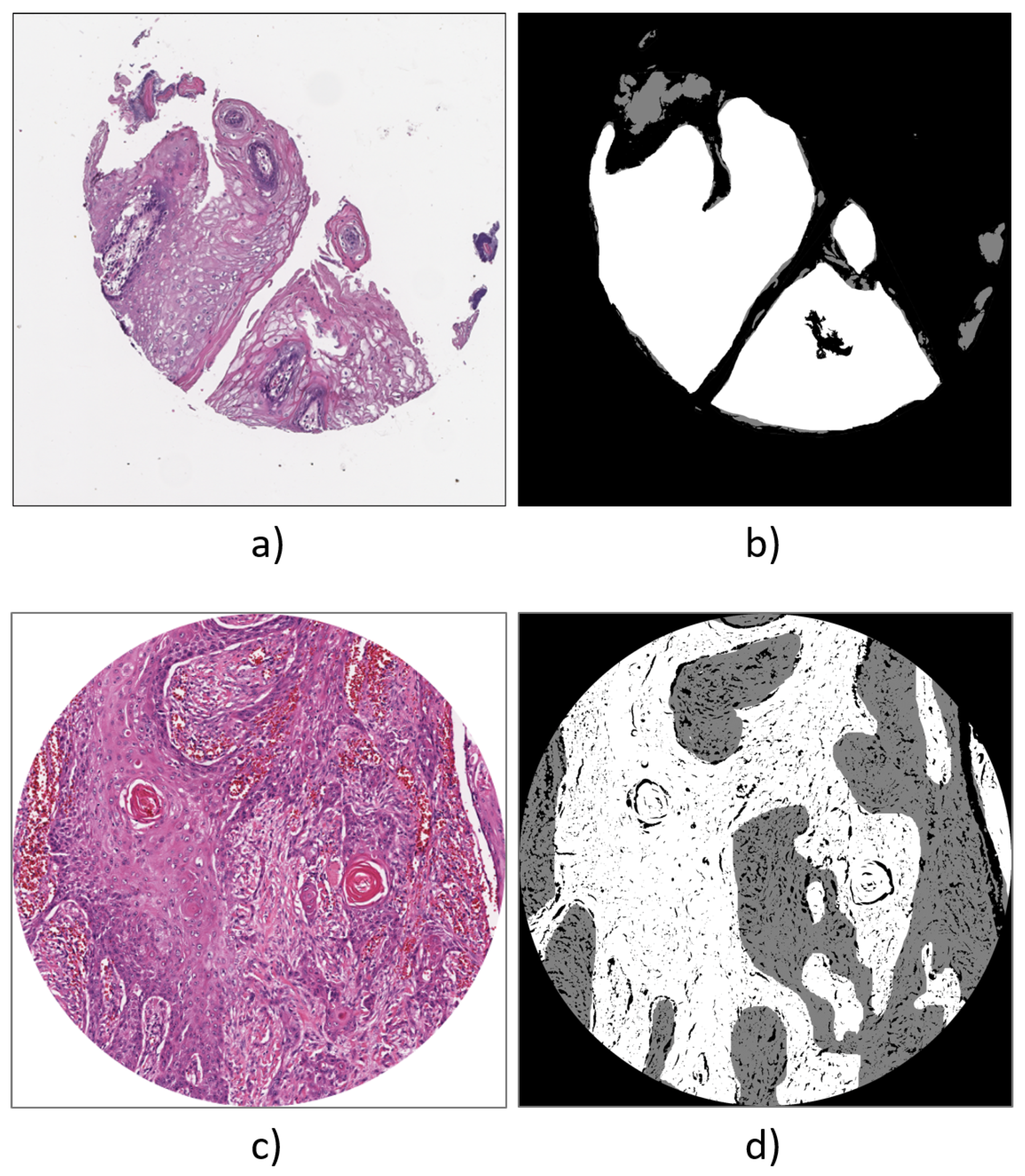
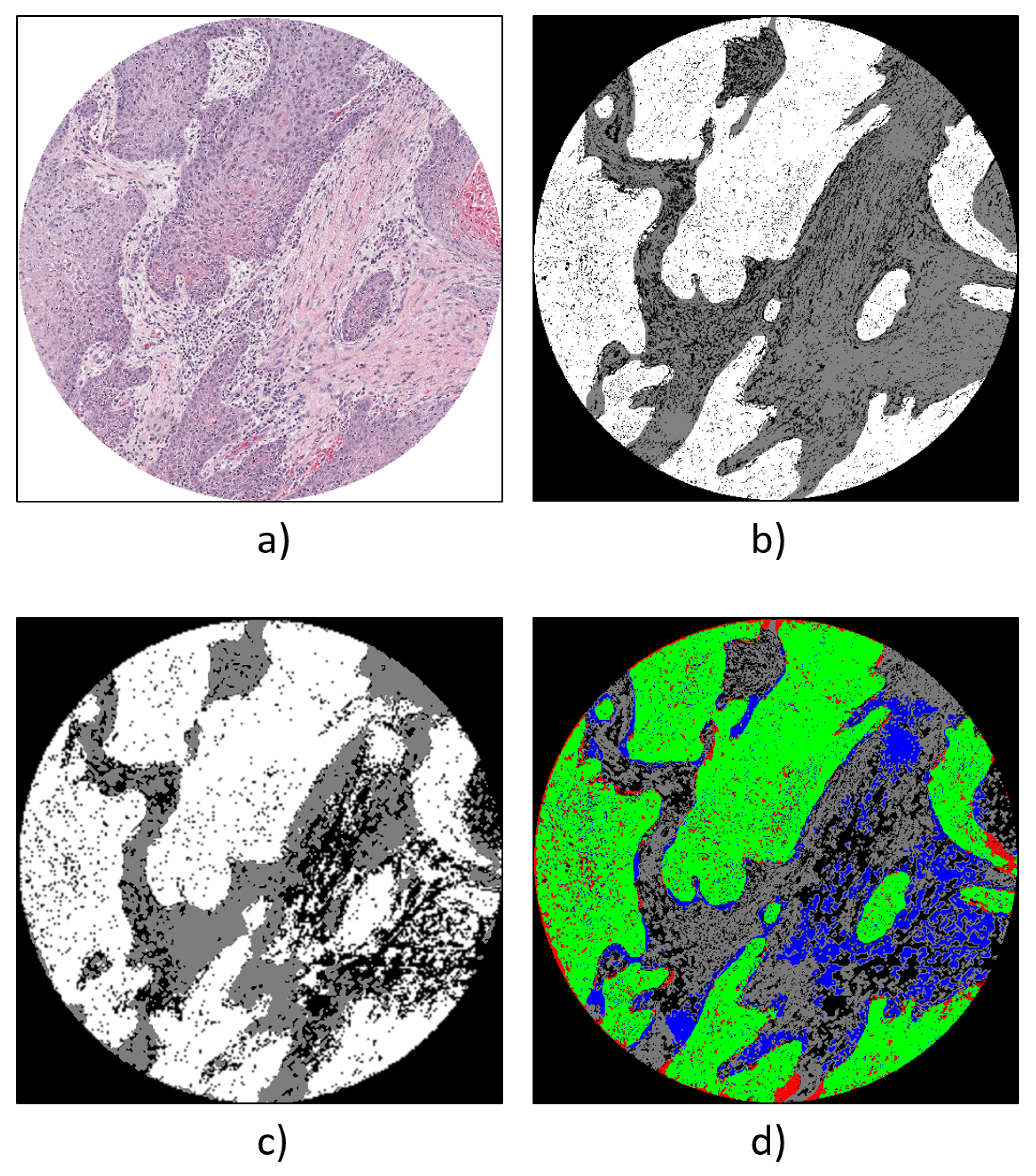
- Carcinoma pixels;
- Tissue pixels not belonging to a carcinoma;
- Non-tissue pixels.
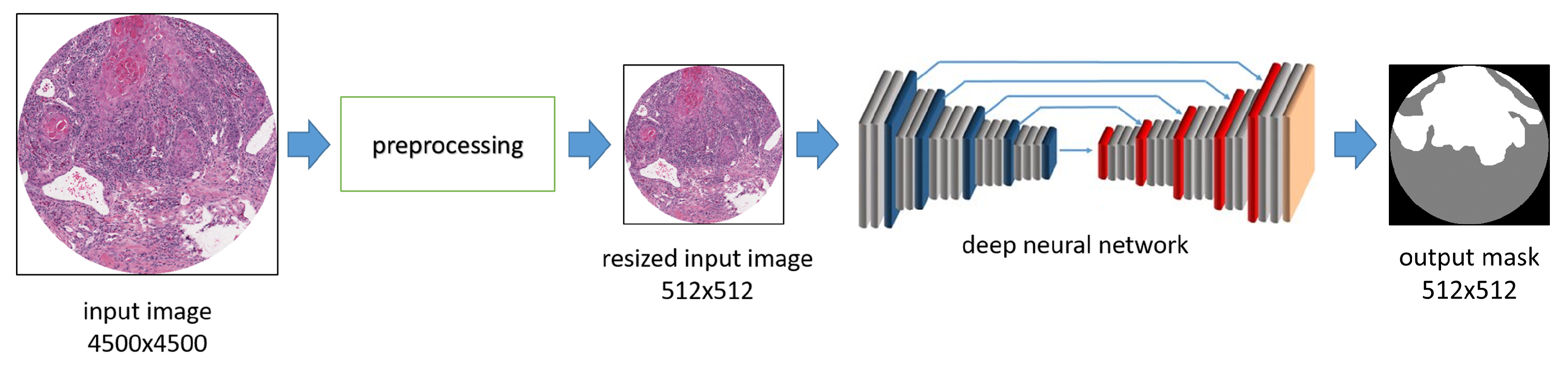
- Simple resizing, where the original input WSI sample is resized from 4500 × 4500 to 512 × 512 pixels without any other change in the color model.
- Color model change, where the WSI sample is resized to 512 × 512 pixels and the original color model is modified. For example, we tested as input for the deep neural network the use of the Red channel of the RGB model in combination with the Hue channel of the HSV model.
3.1. Network Architectures
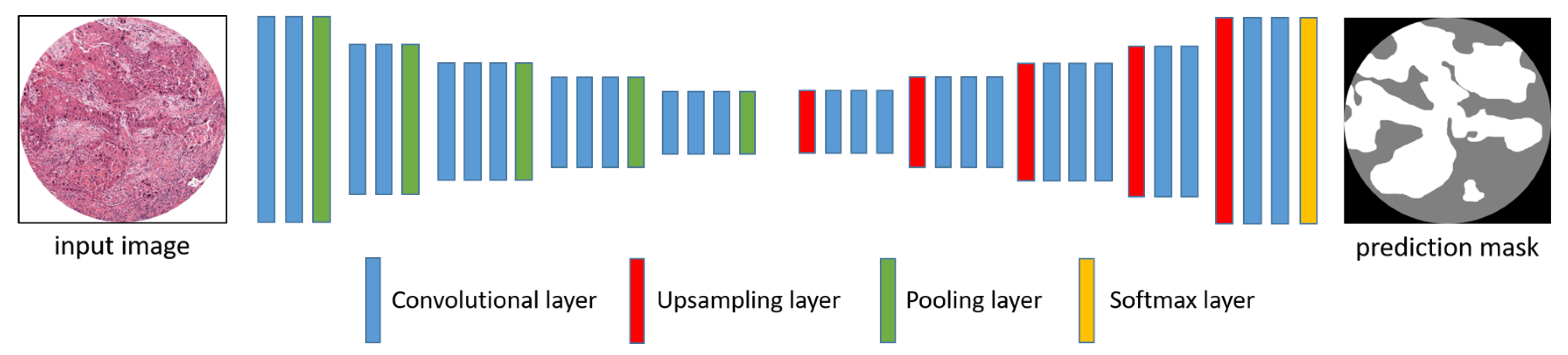
3.1.1. Segnet
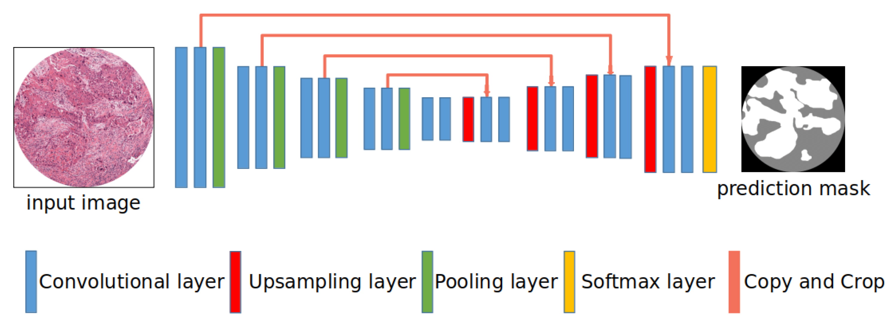
3.1.2. U-Net
3.1.3. U-Net with Different Encoders
3.2. Training and Test
- Carcinoma pixels, colored in white.
- Tissue pixels not belonging to a carcinoma, colored in grey.
- Non-tissue pixels, colored in black.
3.2.1. Training Data
3.2.2. ORCA Dataset
4. Experimental Results
- SegNet.
- U-Net.
- U-Net with VGG16 encoder.
- U-Net with ResNet50 encoder.
- Using RGB images as input;
- Taking into account the HSV color representation and concatenating the Hue channel with the Red channel from the RGB space;
- Using the Red and Value channels.
4.1. Qualitative Evaluation
4.2. Quantitative Results
4.3. Discussion
5. Conclusions
Author Contributions
Funding
Acknowledgments
Conflicts of Interest
References
- Ettinger, K.S.; Ganry, L.; Fernandes, R.P. Oral Cavity Cancer. Oral Maxillofac. Surg. Clin. N. Am. 2019, 31, 13–29. [Google Scholar] [CrossRef]
- The Global Cancer Observatory. Available online: https://gco.iarc.fr/ (accessed on 9 October 2020).
- Bray, F.; Ferlay, J.; Soerjomataram, I.; Siegel, R.L.; Torre, L.A.; Jemal, A. Global cancer statistics 2018: GLOBOCAN estimates of incidence and mortality worldwide for 36 cancers in 185 countries. CA Cancer J. Clin. 2018, 68, 394–424. [Google Scholar] [CrossRef] [PubMed]
- Pantanowitz, L.; Evans, A.; Pfeifer, J.; Collins, L.; Valenstein, P.; Kaplan, K.; Wilbur, D.; Colgan, T. Review of the current state of whole slide imaging in pathology. J. Pathol. Inform. 2011, 2, 36. [Google Scholar] [CrossRef] [PubMed]
- Helin, H.; Tolonen, T.; Ylinen, O.; Tolonen, P.; Näpänkangas, J.; Isola, J. Optimized JPEG 2000 compression for efficient storage of histopathological whole-Slide images. J. Pathol. Inform. 2018, 9. [Google Scholar] [CrossRef]
- Hanna, M.G.; Reuter, V.E.; Hameed, M.R.; Tan, L.K.; Chiang, S.; Sigel, C.; Hollmann, T.; Giri, D.; Samboy, J.; Moradel, C.; et al. Whole slide imaging equivalency and efficiency study: Experience at a large academic center. Mod. Pathol. 2019, 32, 916–928. [Google Scholar] [CrossRef]
- Griffin, J.; Treanor, D. Digital pathology in clinical use: Where are we now and what is holding us back? Histopathology 2017, 70, 134–145. [Google Scholar] [CrossRef]
- Dimitriou, N.; Arandjelović, O.; Caie, P.D. Deep Learning for Whole Slide Image Analysis: An Overview. Front. Med. 2019, 6, 264. [Google Scholar] [CrossRef]
- Xu, H.; Park, S.; Hwang, T.H. Computerized Classification of Prostate Cancer Gleason Scores from Whole Slide Images. IEEE/ACM Trans. Comput. Biol. Bioinform. 2019. [Google Scholar] [CrossRef]
- Tian, K.; Rubadue, C.A.; Lin, D.I.; Veta, M.; Pyle, M.E.; Irshad, H.; Heng, Y.J. Automated clear cell renal carcinoma grade classification with prognostic significance. PLoS ONE 2019, 14. [Google Scholar] [CrossRef]
- Jaber, M.I.; Song, B.; Taylor, C.; Vaske, C.J.; Benz, S.C.; Rabizadeh, S.; Soon-Shiong, P.; Szeto, C.W. A deep learning image-based intrinsic molecular subtype classifier of breast tumors reveals tumor heterogeneity that may affect survival. Breast Cancer Res. 2020, 22. [Google Scholar] [CrossRef]
- Tang, Z.; Chuang, K.V.; DeCarli, C.; Jin, L.W.; Beckett, L.; Keiser, M.J.; Dugger, B.N. Interpretable classification of Alzheimer’s disease pathologies with a convolutional neural network pipeline. Nat. Commun. 2019, 10. [Google Scholar] [CrossRef]
- Guo, Z.; Liu, H.; Ni, H.; Wang, X.; Su, M.; Guo, W.; Wang, K.; Jiang, T.; Qian, Y. A Fast and Refined Cancer Regions Segmentation Framework in Whole-slide Breast Pathological Images. Sci. Rep. 2019, 9. [Google Scholar] [CrossRef]
- Nielsen, F.S.; Pedersen, M.J.; Olsen, M.V.; Larsen, M.S.; Røge, R.; Jørgensen, A.S. Automatic Bone Marrow Cellularity Estimation in H&E Stained Whole Slide Images. Cytom. Part A 2019, 95, 1066–1074. [Google Scholar] [CrossRef]
- Bueno, G.; Fernandez-Carrobles, M.M.; Gonzalez-Lopez, L.; Deniz, O. Glomerulosclerosis identification in whole slide images using semantic segmentation. Comput. Methods Programs Biomed. 2020, 184. [Google Scholar] [CrossRef]
- Mahmood, H.; Shaban, M.; Indave, B.I.; Santos-Silva, A.R.; Rajpoot, N.; Khurram, S.A. Use of artificial intelligence in diagnosis of head and neck precancerous and cancerous lesions: A systematic review. Oral Oncol. 2020, 110, 104885. [Google Scholar] [CrossRef]
- Sun, Y.N.; Wang, Y.Y.; Chang, S.C.; Wu, L.W.; Tsai, S.T. Color-based tumor tissue segmentation for the automated estimation of oral cancer parameters. Microsc. Res. Tech. 2009, 73. [Google Scholar] [CrossRef]
- Rahman, T.Y.; Mahanta, L.B.; Chakraborty, C.; Das, A.K.; Sarma, J.D. Textural pattern classification for oral squamous cell carcinoma. J. Microsc. 2018, 269, 85–93. [Google Scholar] [CrossRef]
- Fouad, S.; Randell, D.; Galton, A.; Mehanna, H.; Landini, G. Unsupervised morphological segmentation of tissue compartments in histopathological images. PLoS ONE 2017, 12, e0188717. [Google Scholar] [CrossRef]
- Das, D.K.; Bose, S.; Maiti, A.K.; Mitra, B.; Mukherjee, G.; Dutta, P.K. Automatic identification of clinically relevant regions from oral tissue histological images for oral squamous cell carcinoma diagnosis. Tissue Cell 2018, 53, 111–119. [Google Scholar] [CrossRef]
- Baik, J.; Ye, Q.; Zhang, L.; Poh, C.; Rosin, M.; MacAulay, C.; Guillaud, M. Automated classification of oral premalignant lesions using image cytometry and Random Forests-based algorithms. Cell. Oncol. 2014, 37. [Google Scholar] [CrossRef]
- Krishnan, M.M.R.; Venkatraghavan, V.; Acharya, U.R.; Pal, M.; Paul, R.R.; Min, L.C.; Ray, A.K.; Chatterjee, J.; Chakraborty, C. Automated oral cancer identification using histopathological images: A hybrid feature extraction paradigm. Micron 2012, 43. [Google Scholar] [CrossRef]
- Krishnan, M.M.R.; Shah, P.; Chakraborty, C.; Ray, A.K. Statistical analysis of textural features for improved classification of oral histopathological images. J. Med. Syst. 2012, 36, 865–881. [Google Scholar] [CrossRef]
- Krishnan, M.M.R.; Choudhary, A.; Chakraborty, C.; Ray, A.K.; Paul, R.R. Texture based segmentation of epithelial layer from oral histological images. Micron 2011, 42. [Google Scholar] [CrossRef]
- Krishnan, M.M.R.; Pal, M.; Bomminayuni, S.K.; Chakraborty, C.; Paul, R.R.; Chatterjee, J.; Ray, A.K. Automated classification of cells in sub-epithelial connective tissue of oral sub-mucous fibrosis-An SVM based approach. Comput. Biol. Med. 2009, 39, 1096–1104. [Google Scholar] [CrossRef]
- Mookiah, M.R.K.; Shah, P.; Chakraborty, C.; Ray, A.K. Brownian motion curve-based textural classification and its application in cancer diagnosis. Anal. Quant. Cytol. Histol. 2011, 33, 158–168. [Google Scholar]
- Martino, F.; Varricchio, S.; Russo, D.; Merolla, F.; Ilardi, G.; Mascolo, M.; Dell’aversana, G.O.; Califano, L.; Toscano, G.; Pietro, G.D.; et al. A machine-learning approach for the assessment of the proliferative compartment of solid tumors on hematoxylin-eosin-stained sections. Cancers 2020, 12, 1344. [Google Scholar] [CrossRef]
- Graham, S.; Vu, Q.D.; Raza, S.E.; Azam, A.; Tsang, Y.W.; Kwak, J.T.; Rajpoot, N. Hover-Net: Simultaneous segmentation and classification of nuclei in multi-tissue histology images. Med. Image Anal. 2019, 58, 101563. [Google Scholar] [CrossRef]
- Raza, S.E.; Cheung, L.; Shaban, M.; Graham, S.; Epstein, D.; Pelengaris, S.; Khan, M.; Rajpoot, N.M. Micro-Net: A unified model for segmentation of various objects in microscopy images. Med. Image Anal. 2019, 52, 160–173. [Google Scholar] [CrossRef]
- Rahman, T.Y.; Mahanta, L.B.; Das, A.K.; Sarma, J.D. Automated oral squamous cell carcinoma identification using shape, texture and color features of whole image strips. Tissue Cell 2020, 63. [Google Scholar] [CrossRef]
- Fraz, M.M.; Khurram, S.A.; Graham, S.; Shaban, M.; Hassan, M.; Loya, A.; Rajpoot, N.M. FABnet: Feature attention-based network for simultaneous segmentation of microvessels and nerves in routine histology images of oral cancer. Neural Comput. Appl. 2020, 32, 9915–9928. [Google Scholar] [CrossRef]
- Shaban, M.; Khurram, S.A.; Fraz, M.M.; Alsubaie, N.; Masood, I.; Mushtaq, S.; Hassan, M.; Loya, A.; Rajpoot, N.M. A Novel Digital Score for Abundance of Tumour Infiltrating Lymphocytes Predicts Disease Free Survival in Oral Squamous Cell Carcinoma. Sci. Rep. 2019, 9, 1–13. [Google Scholar] [CrossRef]
- Litjens, G.; Bandi, P.; Bejnordi, B.E.; Geessink, O.; Balkenhol, M.; Bult, P.; Halilovic, A.; Hermsen, M.; van de Loo, R.; Vogels, R.; et al. 1399 H&E-stained sentinel lymph node sections of breast cancer patients: The CAMELYON dataset. GigaScience 2018, 7, 1–8. [Google Scholar] [CrossRef]
- The Cancer Genome Atlas (TCGA). Available online: https://www.cancer.gov/about-nci/organization/ccg/research/structural-genomics/tcga (accessed on 9 October 2020).
- Weinstein, J.N.; The Cancer Genome Atlas Research Network; Collisson, E.A.; Mills, G.B.; Shaw, K.R.; Ozenberger, B.A.; Ellrott, K.; Shmulevich, I.; Sander, C.; Stuart, J.M. The cancer genome atlas pan-cancer analysis project. Nat. Genet. 2013, 45, 1113–1120. [Google Scholar] [CrossRef] [PubMed]
- Badrinarayanan, V.; Kendall, A.; Cipolla, R. SegNet: A Deep Convolutional Encoder-Decoder Architecture for Image Segmentation. IEEE Trans. Pattern Anal. Mach. Intell. 2017, 39, 2481–2495. [Google Scholar]
- Ronneberger, O.; Fischer, P.; Brox, T. U-Net: Convolutional Networks for Biomedical Image Segmentation. In Proceedings of the International Conference on Medical Image Computing and Computer-Assisted Intervention, Munich, Germany, 5–9 October 2015; pp. 234–241. [Google Scholar]
- Simonyan, K.; Zisserman, A. Very Deep Convolutional Networks for Large-Scale Image Recognition. In Proceedings of the International Conference on Learning Representations, San Diego, CA, USA, 7–9 May 2015. [Google Scholar]
- He, K.; Zhang, X.; Ren, S.; Sun, J. Deep Residual Learning for Image Recognition. In Proceedings of the IEEE Conference on Computer Vision and Pattern Recognition (CVPR), Las Vegas, NV, USA, 27–30 June 2016. [Google Scholar]
- The National Cancer Institute (NCI). Available online: https://www.cancer.gov/ (accessed on 25 September 2020).
- Janocha, K.; Czarnecki, W.M. On Loss Functions for Deep Neural Networks in Classification. arXiv 2017, arXiv:1702.05659. [Google Scholar]
- Sainath, T.N.; Kingsbury, B.; Soltau, H.; Ramabhadran, B. Optimization Techniques to Improve Training Speed of Deep Neural Networks for Large Speech Tasks. IEEE Trans. Audio Speech Lang. Process. 2013, 21, 2267–2276. [Google Scholar]
- Fawakherji, M.; Potena, C.; Pretto, A.; Bloisi, D.D.; Nardi, D. Multi-Spectral Image Synthesis for Crop/Weed Segmentation in Precision Farming. arXiv 2020, arXiv:2009.05750. [Google Scholar]


| Training | SSN | MIoU | IOU | ||
|---|---|---|---|---|---|
| Input | Type | Non-Tissue | Tissue Non-Carcinoma | Carcinoma | |
| RGB | SegNet | 0.51 | 0.74 | 0.49 | 0.30 |
| U-Net | 0.58 | 0.79 | 0.52 | 0.45 | |
| U-Net + VGG16 | 0.64 | 0.84 | 0.56 | 0.45 | |
| U-Net + ResNet50 | 0.67 | 0.85 | 0.59 | 0.56 | |
| Red + Hue | SegNet | 0.49 | 0.70 | 0.48 | 0.30 |
| U-Net | 0.55 | 0.78 | 0.50 | 0.38 | |
| U-Net + VGG16 | 0.33 | 0.22 | 0.28 | 0.53 | |
| U-Net + ResNet50 | 0.57 | 0.80 | 0.48 | 0.43 | |
| Red + Value | SegNet | 0.54 | 0.72 | 0.49 | 0.40 |
| U-Net | 0.57 | 0.78 | 0.49 | 0.46 | |
| U-Net + VGG16 | 0.62 | 0.79 | 0.50 | 0.55 | |
| U-Net + ResNet50 | 0.63 | 0.80 | 0.52 | 0.56 | |
Publisher’s Note: MDPI stays neutral with regard to jurisdictional claims in published maps and institutional affiliations. |
© 2020 by the authors. Licensee MDPI, Basel, Switzerland. This article is an open access article distributed under the terms and conditions of the Creative Commons Attribution (CC BY) license (http://creativecommons.org/licenses/by/4.0/).
Share and Cite
Martino, F.; Bloisi, D.D.; Pennisi, A.; Fawakherji, M.; Ilardi, G.; Russo, D.; Nardi, D.; Staibano, S.; Merolla, F. Deep Learning-Based Pixel-Wise Lesion Segmentation on Oral Squamous Cell Carcinoma Images. Appl. Sci. 2020, 10, 8285. https://doi.org/10.3390/app10228285
Martino F, Bloisi DD, Pennisi A, Fawakherji M, Ilardi G, Russo D, Nardi D, Staibano S, Merolla F. Deep Learning-Based Pixel-Wise Lesion Segmentation on Oral Squamous Cell Carcinoma Images. Applied Sciences. 2020; 10(22):8285. https://doi.org/10.3390/app10228285
Chicago/Turabian StyleMartino, Francesco, Domenico D. Bloisi, Andrea Pennisi, Mulham Fawakherji, Gennaro Ilardi, Daniela Russo, Daniele Nardi, Stefania Staibano, and Francesco Merolla. 2020. "Deep Learning-Based Pixel-Wise Lesion Segmentation on Oral Squamous Cell Carcinoma Images" Applied Sciences 10, no. 22: 8285. https://doi.org/10.3390/app10228285
APA StyleMartino, F., Bloisi, D. D., Pennisi, A., Fawakherji, M., Ilardi, G., Russo, D., Nardi, D., Staibano, S., & Merolla, F. (2020). Deep Learning-Based Pixel-Wise Lesion Segmentation on Oral Squamous Cell Carcinoma Images. Applied Sciences, 10(22), 8285. https://doi.org/10.3390/app10228285