Article

An Efficient Lightweight CNN and Ensemble Machine Learning Classification of Prostate Tissue Using Multilevel Feature Analysis

1
Department of Computer Engineering, u-AHRC, Inje University, Gimhae 50834, Korea
2
Department of Digital Anti-Aging Healthcare, Inje University, Gimhae 50834, Korea
3
Department of Pathology, Yonsei University Hospital, Seoul 03722, Korea
*
Author to whom correspondence should be addressed.
Appl. Sci. 2020, 10(22), 8013; https://doi.org/10.3390/app10228013
Submission received: 23 September 2020 / Revised: 9 November 2020 / Accepted: 10 November 2020 / Published: 12 November 2020
(This article belongs to the Special Issue Machine Learning/Deep Learning in Medical Image Processing)

Abstract

:
Prostate carcinoma is caused when cells and glands in the prostate change their shape and size from normal to abnormal. Typically, the pathologist’s goal is to classify the staining slides and differentiate normal from abnormal tissue. In the present study, we used a computational approach to classify images and features of benign and malignant tissues using artificial intelligence (AI) techniques. Here, we introduce two lightweight convolutional neural network (CNN) architectures and an ensemble machine learning (EML) method for image and feature classification, respectively. Moreover, the classification using pre-trained models and handcrafted features was carried out for comparative analysis. The binary classification was performed to classify between the two grade groups (benign vs. malignant) and quantile-quantile plots were used to show their predicted outcomes. Our proposed models for deep learning (DL) and machine learning (ML) classification achieved promising accuracies of 94.0% and 92.0%, respectively, based on non-handcrafted features extracted from CNN layers. Therefore, these models were able to predict nearly perfectly accurately using few trainable parameters or CNN layers, highlighting the importance of DL and ML techniques and suggesting that the computational analysis of microscopic anatomy will be essential to the future practice of pathology.

1. Introduction

Image classification and analysis has become popular in recent years, especially for medical images. Cancer diagnosis and grading are often performed and evaluated using AI as these processes have become increasingly complex, because of growth in cancer incidence and the numbers of specific treatments. The analysis and classification of prostate cancer (PCa) are among the most challenging and difficult. PCa is the second most commonly diagnosed cancer among men in the USA and Europe, affecting approximately 25% of patients with cancer in the Western world [1]. PCa is a type of cancer that has always been an important challenge for pathologists and medical practitioners, with respect to detection, analysis, diagnosis, and treatment. Recently, researchers have analyzed PCa in young Korean men (<50 years of age), considering the pathological features of radical prostatectomy specimens and biochemical recurrence of PCa [2].
In the United States, thousands of people exhibit PCa. In 2017, there were approximately 161,360 new cases and 26,730 deaths, constituting 19% of all new cancer cases and 8% of all cancer deaths [3]. Therefore, it is important to detect PCa at an early stage to increase the survival rate. Currently, for the clinical diagnosis of PCa, methods that are performed in hospitals include a prostate-specific antigen test, digital rectal exam, trans-rectal ultrasound, and magnetic resonance imaging. Core needle biopsy examination is a common and useful technique, performed by insertion of a thin, hollow needle into the prostate gland to remove a tissue sample [4,5,6]. However, PCa diagnosis via microscopic biopsy images is challenging. Therefore, diagnostic accuracy may vary among pathologists.
Generally, in histopathology sections, pathologists categorize stained microscopy biopsy images into benign and malignant. To carry out PCa grading, pathologists use the Gleason grading system, which was originally based on the sum of the two Gleason scores for the most common so-called Gleason patterns (GPs). Many studies conclude that this is the recommended methodology for grading PCa [7]. The Gleason grading system defines five histological patterns from GP 1 (well differentiated) to GP 5 (poorly differentiated), with a focus on the shapes of atypical glands [8,9,10,11]. During the grossing study, the tumor affected in the prostate gland is extracted by the pathologist for examination under a microscope for cancerous cells [12,13]. In this cell culturing process, the tissues are stained with hematoxylin and eosin (H&E) compounds, yielding a combination of dark blue and bright pink colors, respectively [14,15,16,17,18]. In digital pathology, there are some protocols that every pathologist follows for preparing and staining the tissue slides. However, the acquisition systems and staining process vary from one pathologist to another. The generated tissue images with the variations in colour intensity and artifacts could impact the classification accuracy of the analysis [19,20].
DL and ML in AI have recently shown excellent performance in the classification of medical images. These techniques are used for computer vision tasks (e.g., segmentation, object detection, and image classification) and pattern recognition exploiting handcrafted features from a large-scale database, thus allowing new predictions from existing data [21,22,23,24]. DL is a class of ML algorithms, where multiple layers are used to extract higher-level features gradually from the raw input. ML is a branch of AI concentrated on application building that learns from data. ML algorithms are trained to learn features and patterns in huge amounts of data to make predictions based on new data. Both DL and ML have shown promising results in the field of medical imaging and have the potential to assist pathologists and radiologists with an accurate diagnosis; this may save time and minimize the costs of diagnosis [25,26,27,28]. For image classification, DL models are built to train, validate, and test thousands of images of different types for accurate prediction. These models consist of many layers through which a CNN transforms the images using functions such as convolution, kernel initialization, pooling, activation, padding, batch normalization, and stride.
The combination of image-feature engineering and ML classification has shown remarkable performance in terms of medical image analysis and classification. In contrast, CNN adaptively learns various image features to perform image transformation, focusing on features that are highly predictive for a specific learning objective. For instance, images of benign and malignant tissues could be presented to a network composed of convolutional layers with different numbers of filters that detect computational features and highlight the pixel pattern in each image. Based on these patterns, the network could use sigmoid and softmax classifiers to learn the extracted and important features, respectively. In DL, the “pipeline” of CNN’s processing (i.e., from inputs to any output prediction) is opaque, performed automatically like a passage through a “black box” tunnel, where the user remains fully unaware of the process details. It is difficult to examine a CNN layer-by-layer. Therefore, each layer’s visualization results and prediction mechanism are challenging to interpret.
The present paper proposes a pipeline for tissue image classification using DL and ML techniques. We developed two lightweight CNN (LWCNN) models for automatic detection of the GP in histological sections of PCa and extracted the non-handcrafted texture features from the CNN layers to classify these using an ensemble ML (EML) method. Color pre-processing was performed for enhancing images. To carry out a comparative analysis, the two types of hand-designed [29] features, such as the opposite color local binary patterns (OCLBP) [30] and improved OCLBP (IOCLBP) [30] were extracted and pre-trained models (VGG-16, ResNet-50, Inception-V3, and DenseNet-121) [31] were used for EML and DL classification, respectively. To avoid the complexity and build lightweight DL models, we used a few hidden layers and trainable parameters, and therefore, the models were named LWCNN.
The DL models were trained several times on the same histopathology dataset using different parameters and filters. For each round of training, we fine-tuned the hyperparameters, optimization function, and activation function to improve the model performance, including its accuracy. Binary classification is critical for PCa diagnosis because the goal of the pathologist is to identify whether each tumor is benign or malignant [32]. We generated a class activation map (CAM) using predicted images and created a heat map to visualize the method by which the LWCNN learned to recognize the pixel pattern (image texture) based on activation functions, thus interpreting the decision of the neural network. The CAM visualization results of the training and testing were difficult to interpret because CNNs are black-box models [33,34].

2. Related Work

A CNN was first used on medical images by Lo et al. [35,36]. Their model (LeNet) succeeded in a real-world application and could recognize hand-written digits [37]. Subsequent CNN-based methods showed the potential for automated image classification and prediction, especially after the introduction of AlexNet, a system that won the ImageNet challenge. In this era, the categorizing and auto-detection of cancer in the histological sections using machine assistance have shown excellent performance in the field of early detection of cancer.
Zheng et al. [38] developed a new CNN-based architecture for histopathological images, using the 3D multiparametric MRI data provided by PROSTATEx challenge. Data augmentation was performed through 3D rotation and slicing, to incorporate the 3D information of the lesion. They achieved the second-highest AUC (0.84) in the PROSTATEx challenge, which shows the great potential of deep learning for cancer imaging.
Han et al. [39] used breast cancer samples from the BreaKHis dataset to perform multi-classification using subordinate classes of breast cancer (ductal carcinoma, fibroadenoma, lobular carcinoma, adenosis, Phyllodes tumor, tubular adenoma, mucinous carcinoma, and papillary carcinoma). The author developed a new deep learning model and has achieved remarkable performance with an average accuracy of 93.2% on a large-scale dataset.
Kumar et al. [12] performed k-means segmentation to separate the background cells from the microscopy biopsy images. They extracted morphological and textural features from for automated detection and classification of cancer. They used different types of machine learning classifiers (random forest, Support vector machine, fuzzy k-nearest neighbor, and k-nearest neighbor) to classify connectivity, epithelial, muscular, and nervous tissues. Finally, the author obtained an average accuracy of 92.19% based on their proposed approach using a k-nearest neighbor classifier.
Abraham et al. [40] used multiparametric magnetic resonance images and presented a novel method for the grading of prostate cancer. They used VGG-16 CNN and an ordinal class classifier with J48 as the base classifier. The author used the PROSTATAx-2 2017 grand challenge dataset for their research work. Their method achieved a positive predictive value of 90.8%.
Yoo et al. [3] proposed an automated CNN-based pipeline for prostate cancer detection using diffusion-weighted magnetic resonance imaging (DWI) for each patient. They used a total of 427 patients as the dataset, out of these, 175 with PCa and 252 patients without PCa. The author used five CNNs based on the ResNet architecture and extracted first order statical features for classification. The analysis was carried out based on a slice- and patient-level. Finally, their proposed pipeline achieved the best result (AUC of 87%) using CNN1.
Turki [41] performed machine learning classification for cancer detection and used a data sample of colon, liver, thyroid cancer. They applied different ML algorithms, such as deep boost, AdaBoost, XgBoost, and support vector machines. The performance of the algorithms was evaluated using the area under the curve (AUC) and accuracy on real clinical data used classification.
Veta et al. [42] proposed different methods for the analysis of breast cancer histopathology images. They discussed different techniques for tissue image analysis and processing like tissue components segmentation, nuclei detection, tubules segmentation, mitotic detection, and computer-aided diagnosis. Before discussing the different image analysis algorithms, the author gave an overview of the tissue preparation, slide staining processes, and digitization of histological slides. In this paper, their approach is to perform clustering or supervised classification to acquire binary or probability maps for the different stains.
Moradi et al. [43] performed prostate cancer detection based on different image analysis techniques. The author used ultrasound, MRI, and histopathology images, and among these, ultrasound images were selected for cancer detection. For the classification of prostate cancer, feature extraction was carried out using the ultrasound echo radio-frequency (RF) signals, B-scan images, and Doppler images.
Alom et al. [44] proposed a deep CNN (DCNN) model for breast cancer classification. The model was developed based on the three powerful CNN architecture by combining the strength of the inception network (Inception-v4), the residual network (ResNet), and the recurrent convolutional neural network (RCNN). Thus, their proposed model was named as inception recurrent residual convolution neural network (IRRCNN). They used two publicly available datasets including BreakHis and Breast Cancer (BC) classification challenge 2015. The test results were compared against the existing state-of-art models for image-based, patch-based, image-level, and patient-level classification.
Wang et al. [45] proposed a novel method for the classification of colorectal cancer histopathological images. The author developed a novel bilinear convolutional neural network (BCNN) model that consists of two CNNs, and the outputs of the CNN layers are multiplied with the outer product at each spatial domain. Color deconvolution was performed to separate the tissue components (hematoxylin and eosin) for BCNN classification. Their proposed model performed better than the traditional CNN by classifying colorectal cancer images into eight different classes.
Bianconi et al. [20] compared the combination effect of six different colour pre-processing methods and 12 colour texture features on the patch-based classification of H&E stained images. They found that classification performance was poor using the generated colour descriptors. However, they achieved promising results using some pre-processing methods such as co-occurrence matrices, Gabor filters, and Local Binary Patterns.
Kather et al. [31] investigated the usefulness of image texture features, pre-trained convolutional networks against variants of local binary patterns for classifying different types of tissue sub-regions, namely stroma, epithelium, necrosis, and lymphocytes. They used seven different datasets of histological images for classifying the handcrafted and non-handcrafted features using standard classifiers (e.g., support vector machines) to obtain overall accuracy between 95% and 99%.

3. Tissue Staining and Data Collection

3.1. Tissue Staining

For the identification of cancerous cells, the prostate tissue was sectioned with a thickness of 4 μ m . The process of deparaffinization (i.e., removal of paraffin wax from slides prior to staining) is especially important after tissue sectioning because, otherwise, only poor staining may be achieved. However, in practice, each tissue section was deparaffinized and rehydrated in an appropriate manner and H&E staining was carried out successfully using an automated stainer (Autostainer XL, Leica). Hematoxylin and Eosin are positively and negatively charged, respectively. The nucleic acids in the nucleus are negatively charged components of basophilic cells; hematoxylin reacts with these components. Amino groups in proteins in the cytoplasm are positively charged components of acidophilic cells; eosin reacts with these components [46,47,48]. Figure 1 shows the visualization of the H&E stained biopsy image, which was analyzed using QuPath open-source software. The results of H&E staining are shown separately, with their respective chemical formulas.

3.2. Data Collection

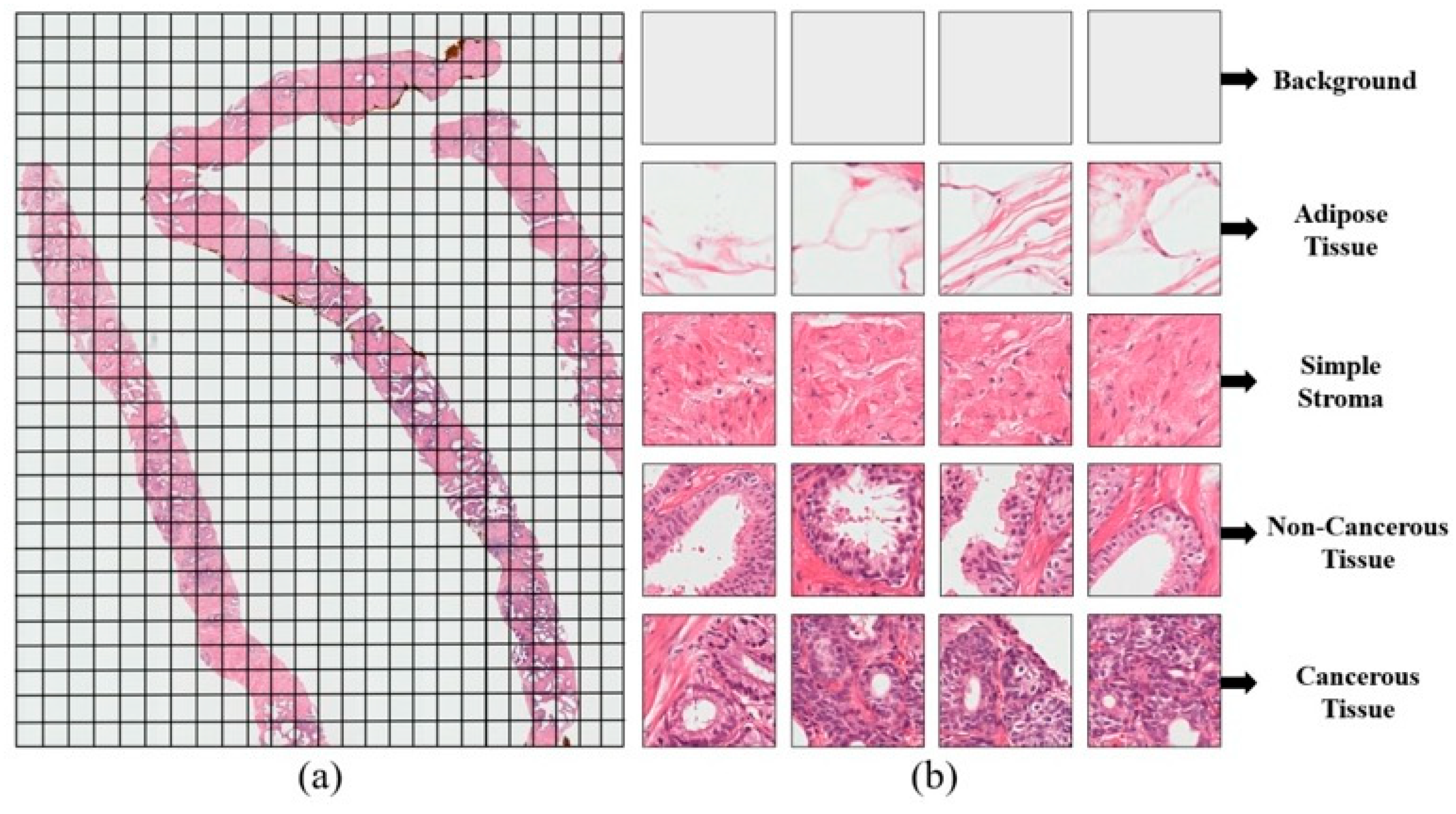
The whole-slide H&E stained images of size 33,584 × 70,352 pixels were acquired from the pathology department of the Severance Hospital of Yonsei University. The slide images were further processed to generate multiple sizes (256 × 256, 512 × 512, and 1024 × 1024) of 2D patches by scanning at 40× optical magnification with 0.3NA objective using a digital camera (Olympus C-3000) which is attached to a microscope (Olympus BX-51). The extracted regions of interest (ROIs) were sent to the pathologist for prostate cancer (PCa) grading. Figure 2 shows an example of the cropped patches extracted from a whole-slide image. Regions containing background and adipose tissue were excluded. After the labeled patches were received, 6000 samples were selected, all with size 256 × 256 pixels (24 bit/pixel); the samples were divided equally into two classes: cancerous and non-cancerous. The tissue samples used in our research were extracted from 10 patients. These samples had an RGB color coding scheme (8 bits each for red, green, and blue).

4. Materials and Methods

4.1. Proposed Pipeline

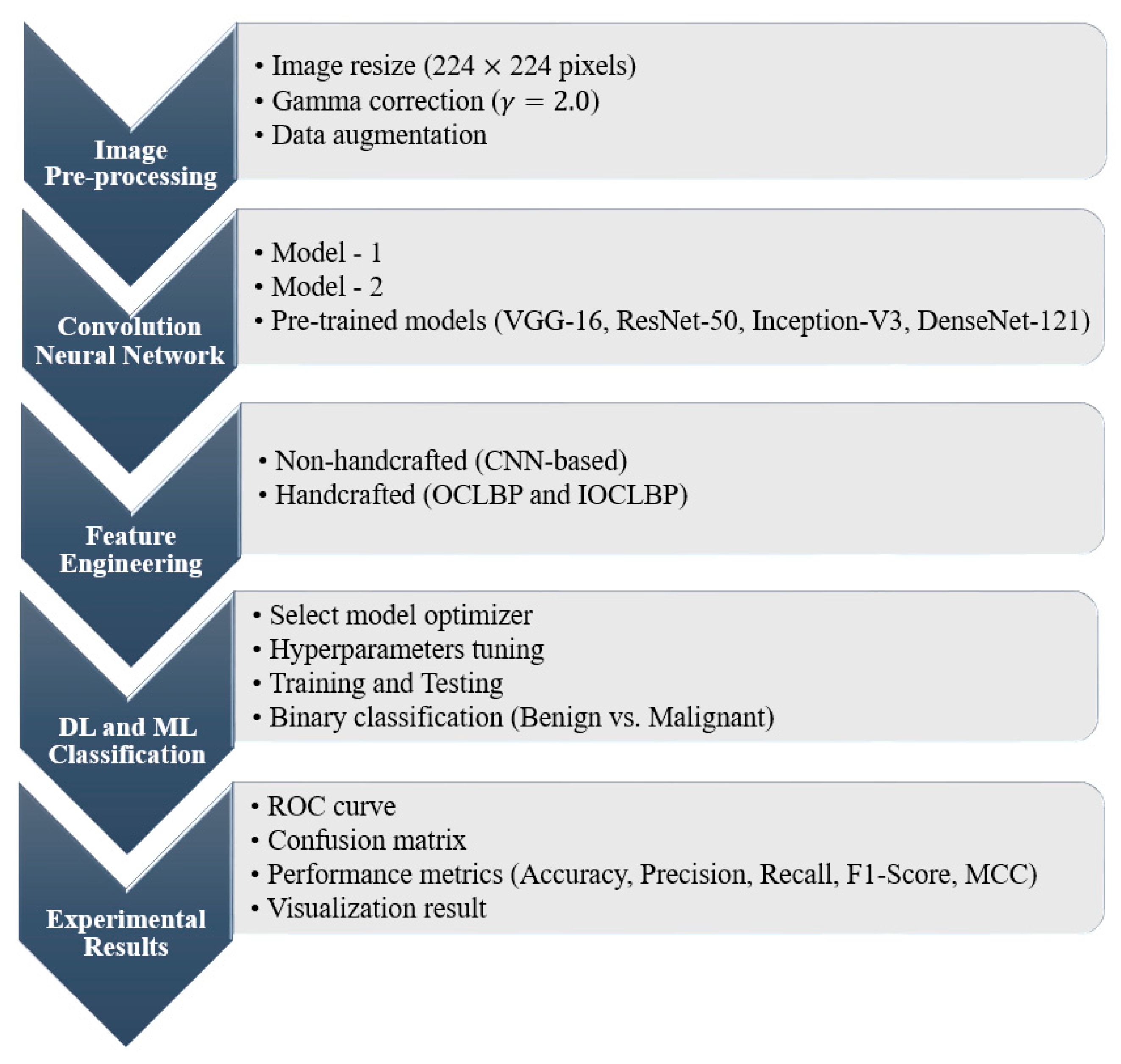
Image and feature classification based on DL and ML methods showed some promising results in categorizing microscopic images of benign or malignant tissues. Our proposed pipeline for this paper is shown in Figure 3. Our analysis of a tissue image dataset was carried out in five phases, which include image pre-processing, analyze CNN models, feature analysis, model classification, and performance evaluation. In this study, we developed two LWCNN models (model 1 and model 2) and used state-of-art pre-trained models to carry out 2D image classification and perform a comparative analysis among the models. Also, EML classification was performed to classify the handcrafted (OCLBP and IOCLBP) and non-handcrafted (CNN-based) colour texture features extracted from tissue images.

4.2. Image Preprocessing

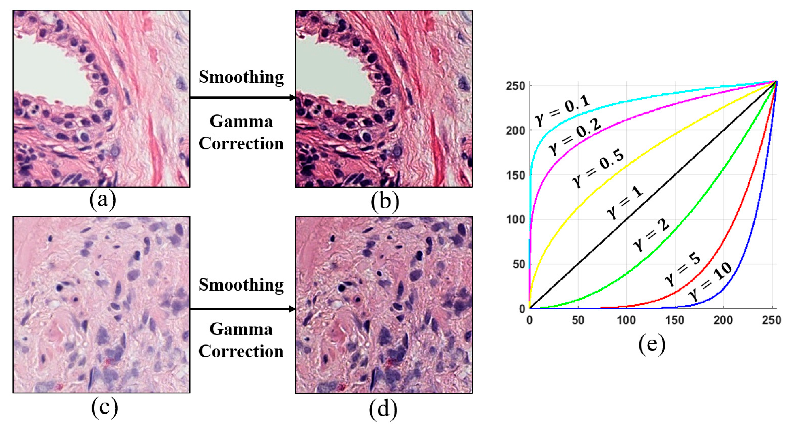
In this phase, the preprocessing was carried out, whereby we resized the patches to 224 × 224 pixels for CNN training, and to adjust the contrast level of the image, power law (gamma) transformation [49,50] was applied to the resized images. The concept of gamma was used to encode and decode luminance values in image systems. Figure 4 illustrates the clarity of images before and after the application of this operation.
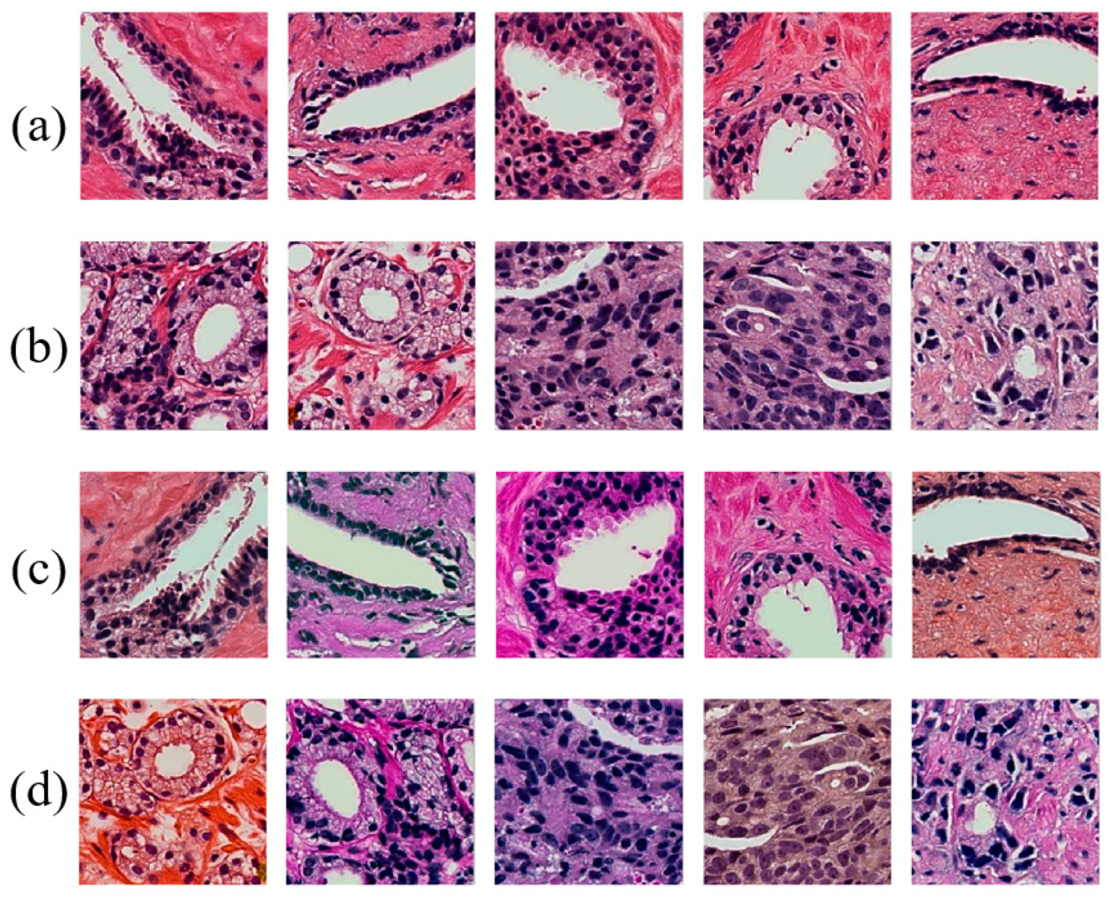
The dataset splitting was performed for training, validating, and testing the CNN models. The data samples were labeled with 0 (non-cancerous) and 1 (cancerous) for accurate classification and randomly assigned to one of three groups for training, validation, and testing, as shown in Table 1. The dataset used for DL and ML classification holds a total of 6000 samples. Out of these, 3600 were used for training, 1200 for validation, and 1200 for testing. Before the samples were fed to the network for classification, data augmentation was performed on the training set, which enabled analysis of model performance, reduction of overfitting problems, and improvement of generalization [51]. Therefore, to create some changes in the images, some transformations were applied using augmentation techniques, and these included rotation by 90 ° , transposition, random_brightening, and random_contrast, random_hue, and random_saturation, shown in Figure 5c,d. Keras and Tensorflow functions were used to execute data augmentation.

4.3. Convolution Neural Network

To classify images of PCa, this paper introduces two LWCNN models to perform the classification of the GP and distinguish between two classes. Both model 1 and model 2 included CNN layers, such as those for input, convolution, rectified linear unit (ReLU), max pooling, dropout, flattening, GAP, and classification. Model 1 contained four convolutional blocks, with a depth of 10 layers, which interleaved two-dimensional (2D) convolutional layers (3 × 3 kernel, strides, and padding) with ReLU and batch normalization (BN) layers, followed by three max-pooling (2 × 2) and three dropout layers. To connect the neural network [52,53], a flattening layer and a sequence of three dense layers containing 1024, 1024, and 2 neurons were connected for feature classification and two probabilistic outputs. The sigmoid activation function [54,55] was used as a binary classifier. The numbers of filters in each block were 32, 64, 128, and 256. These filters acted as a sliding window over the entire image.
Model 2 contained three convolutional blocks, with a depth of seven layers, where the 2D convolutional, ReLU, and BN layers were identical to model 1 but were interleaved with two max-pooling (2 × 2) layers and one dropout layer. The numbers of convolutional filters in this model were 92, 192, and 384. A GAP layer was used instead of flattening, the classification section in this model also had three dense layers containing 64, 32, and 2 neurons. Here, a softmax [56,57] classifier was used to reduce binary loss. The input shape was set to 224 × 224 × 3 while building the model. The detailed design and specification of our lightweight CNN (LWCNN) models are shown in Figure 6 and Table 2, respectively. Model 2 was modified from model 1 based on multilevel feature analysis to improve classification accuracy and reduce validation loss, as shown in Figure 7.
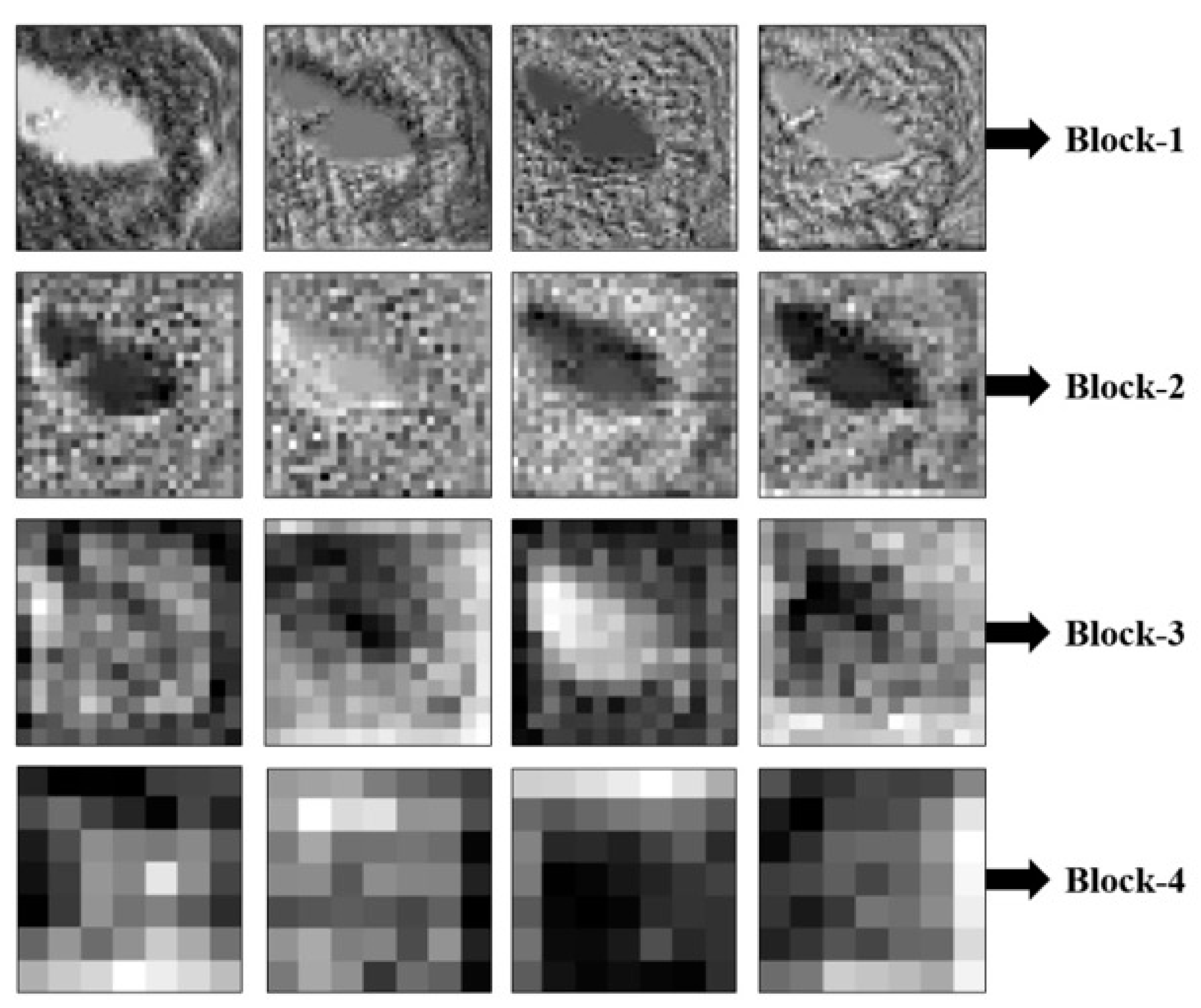
The multilevel feature maps were extracted after each convolutional block for pattern analysis and to understand the pixel distribution that the CNN detected, based on the number of convolution filters applied for edge detection and feature extraction. The convolution operation was performed by sliding the filter or kernel over the input image. Element-wise matrix multiplication was performed at each location in the image matrix and the output results were summed to generate the feature map. Max pooling was applied to reduce the input shape, prevent system memorization, and extract maximum information from each feature map. The feature maps from the first block held most of the information present in the image; that block acted as an edge detector. However, the feature map appeared more similar to an abstract representation and less similar to the original image, with advancement deeper into the network (see Figure 7). In block-3, the image pattern was somewhat visible, and by block-4, it became unrecognizable. This transformation occurred because deeper features encode high-level concepts, such as 2D information regarding the tissue (e.g., only spatial values of 0 or 1), while the CNN detects edges and shapes from low-level feature maps. Therefore, to improve the performance of the LWCNN, based on the observation that block-4 yielded unrecognizable images, model 2 was developed using three convolutional blocks, and selected as the model that this paper proposes.
To validate the performance of model 2 (LWCNN), we also included pre-trained CNN models (VGG-16, ResNet-50, Inceptio-V3, and DenseNet-121) for histopathology image classification. These models are very powerful and effective for extracting and classifying the deep CNN features. For each pre-trained network, the dense or classification block was configured according to the model specification. Sigmoid activation function was used for all the pre-trained models to perform binary classification.

4.4. Feature Engineering

The extraction of texture features based on handcrafted and non-handcrafted was performed for ensemble machine learning (EML) classification. First, non-handcrafted or CNN-based features were extracted from the GAP layer of the proposed LWCNN (model 2). A different number of feature maps were generated from each CNN layer and the GAP mechanism was used to calculate the average value for each feature map. Second, a total of 20 handcrafted colour texture features were extracted using OCLBP and IOCLBP techniques. Out of these, 10 features were extracted using OCLBP, and 10 features using IOCLBP. The hand-designed feature analysis was performed for EML classification and compare with the non-handcrafted features classification results.
After we generate colour texture map, the LBP technique was applied to each colour channel (Red/Green/Blue) of OCLBP and IOCLBP separately. These state-of-art methods are the extensions of local binary patterns (LBP) and effective for colour image analysis. OCLBP and IOCLBP are the intra- and inter-channel descriptors with dissimilar local thresholding scheme (i.e., the peripheral pixels of OCLBP are thresholded at the central pixel value, and IOCLBP thresholding is based on the mean value) [30]. For each aforesaid state-of-art methods, the feature vector was obtained using general rotation-invariant operators (i.e., neighbor set of pixels p was placed on a circle of radius R) that can distinguish the spatial pattern and the contrast of local image texture. Therefore, the operators p = 8 and R = 2 were used to extract the colour features from the H&E stained tissue images.

4.5. DL and ML Classification

Prior to training and testing the LWCNN, pre-trained, and EML [58] models, we fine-tuned different types of parameters for better prediction and to minimize model loss. To compute the feature maps in each convolutional layer, a non-linear activation function (ReLU) was used, and the equation can be defined as:
A i , j , k = max ( w n T I i , j + b n , 0 )
where A i , j , k is the activation value of the nth feature map at the location ( i , j ), I i , j is the input patch, and w n and b n are the weight vector and bias term, respectively, of the nth filter.
BN was also used after each convolution layer to regularize the model, reducing the need for dropout. BN was used in our model because it is more effective than global data normalization. The latter normalization transforms the entire dataset so that it has a mean of zero and unit variance, while BN computes approximations of the mean and variance after each mini-batch. Therefore, BN enables the use of the ReLU activation function without saturating the model. Typically, BN is performed using the following equation:
BN   ( X n o r m a l i z e ) = ( x n μ m b ) / σ m b 2 + c
where x n is the d -dimensional input, μ m b and σ m b 2 are the mean and variance, respectively, of the mini-batch, and c is a constant.
To optimize the weights of the network and analyze the performance of the LWCNN models, we performed a comparative analysis based on four different types of optimizers, namely stochastic gradient descent (SGD), Adadelta, Adam, and RMSprop. The results of comparative analysis are shown in the next section. The classification performance is measured using the cross-entropy loss, or log loss, whose output is a probability value between 0 and 1. To train our network, we used binary cross-entropy. The standard loss function for binary classification is given by:
B i n a r y l o s s = 1 N i = 1 N [ Y i × log ( M w ( X i ) ) + ( 1 Y i ) × log ( 1 M w ( X i ) ) ]
where N is the number of output class, X i and Y i are the input samples and target labels, respectively, and M w is the model with network weight, w .
The hyperparameters were tuned while setting a minimum learning rate of 0.001 using the function known as ReduceLROnPlateau, a factor of 0.8 and patience of 10 were set; thus, if no improvement was observed in validation loss for 10 consecutive epochs, the learning rate was reduced by a factor of 0.8. The batch size was set to eight for training the model and regularization was applied by dropping out 25% and 50% of the weights in the convolution and dense blocks of LWCNN, respectively. The probabilistic output in the dense layer was computed using sigmoid and softmax classifiers.
In addition to CNN methods, traditional ML algorithms including logistic regression (LR) [59] and random forest (RF) [60] were used for features classification. In this paper, an ensemble voting method was proposed in which LR and RF classifiers were combined to create an EML model. This ensemble technique was used to classify the handcrafted and non-handcrafted features and compare the classification performance. The LWCNN, pre-trained, and EML models were tested using the unknown or unseen data samples. Typically, for ML classification, cross-validation was used by splitting the training data into k-fold (i.e., k = 5) to determine the model generalizability, and the result was computed by averaging the accuracies from each of the k trials. Prior to ML classification [61,62,63], the feature values for training and testing were normalized using the standard normal distribution function, which can be expressed as:
P i _ N o r m a l i s e d = P i μ σ
where P i is the i th pixel in an individual tissue image, and μ and σ are the mean and standard deviation of the dataset.
The DL and ML models were built with the Python 3 programming language using the Keras and Tensorflow libraries. Approximately 36 h were invested in fine-tuning the hyperparameters to achieve better accuracy. Figure 8 shows the entire process flow diagram for DL and ML classification. The hyperparameters that were used for DL and ML models are shown in Table 3.
The models were trained, validated, and tested on a PC with the following specifications: an Intel corei7 CPU (2.93 GHz), one NVIDIA GeForce RTX 2080 GPU, and 24 GB of RAM.

5. Experimental Results

This study mainly focuses on image classification based on AI. The proposed LWCNN (model 2) for tissue image classification and EML for feature classification produced reliable results, which met our requirements, at an acceptable speed. To develop DL models, a CNN approach was used as it is proven excellent performance in detecting specific regions for multiclass and binary classification. When splitting the dataset, a ratio of 8:2 was set for training and testing. Moreover, to validate the model after each epoch, the training set was further divided, such that 75% of the data was allocated for training and 25% was allocated for validation. Five-fold cross-validation was used during EML training. Algorithms used for preprocessing, data analysis, and classification were implemented in the MATLAB R2019a and PyCharm environments.

5.1. Performance Analysis

In this study, a binary classification approach was used to classify benign and malignant samples of prostate tissue. Two levels of classification were performed: DL (based on images) and ML (based on features). Table 4 shows the comparative analysis between the optimizers for model 1 and model 2, respectively. The developed LWCNN models were trained a couple of times by changing the optimizers during training.
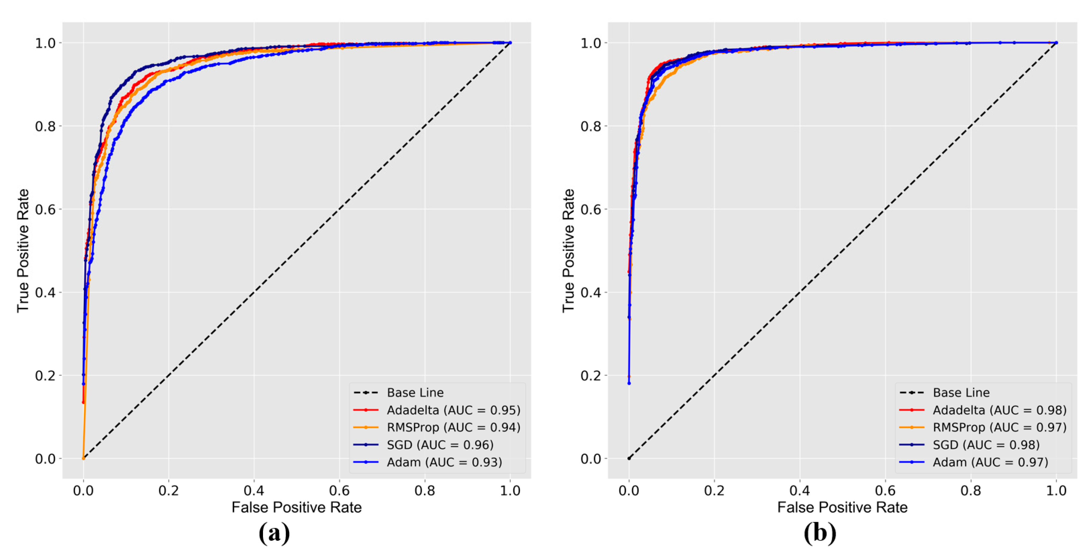
From the above comparison table, we can analyze that the Adadelta performed the best and gave the best accuracies on test data for both the architectures. SGD and Adam performed close to Adadelta for model 2. On the other hand, RMSProp performed close to Adadelta for model 1. However, Adadelta (update version of Adam and Adagrad) is a more robust optimizer that restricts the window of accumulated past gradients to some fixed size w instead of accumulating all past square gradients. The comparison of these optimizers revealed that Aadelta is more stable and more rapid, hence, an overall improvement on SGD, RMSProp, and Adam. The behavior and performance of the optimizers were analyzed using the receiver operating characteristic (ROC) curve. It is a probabilistic curve that represents the diagnostic ability of a binary classifier system, including an indication of its effective threshold value. The area under the ROC curve (AUC) summarizes the extent to which a model can separate the two classes. Figure 9a,b show the ROC curve and corresponding AUC that depicts the effectiveness of different optimizers used for model 1 and model 2, respectively. For model 1, the AUCs were 0.95, 0.94, 0.96, and 0.93, and for model 2, 0.98, 0.97, 0.98, and 0.97 were obtained using Adadelta, RMSProp, SGD, and Adam, respectively.
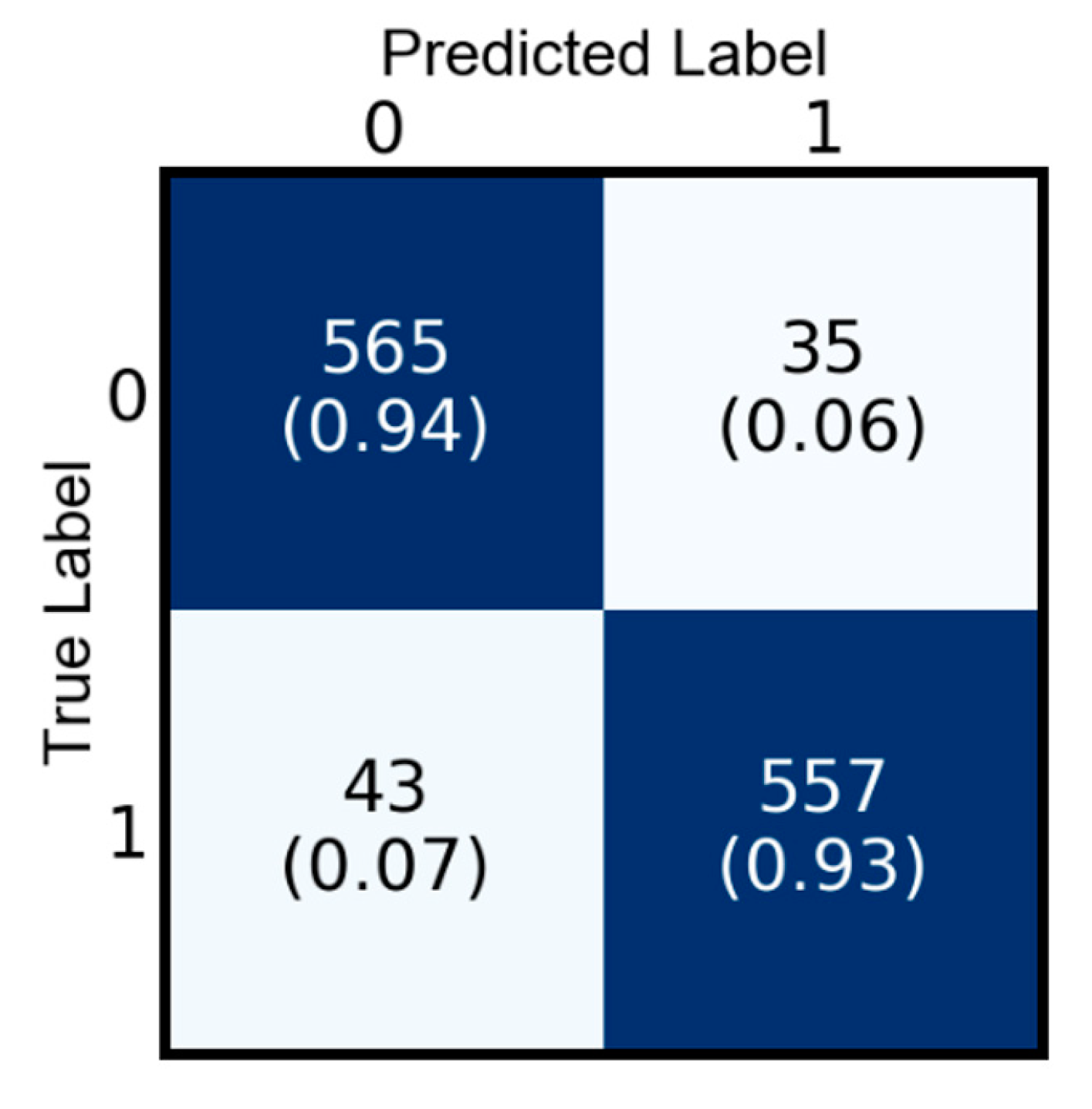
Further, based on the optimum accuracy in Table 4, we carried out EML classification using the CNN extracted features from model 2, to analyze the efficiency of ML algorithms. Also, handcrafted features classification was performed to compare the performance with the non-handcrafted features classification results. Moreover, the EML model achieved promising results using the CNN-based features. Model 2 outperformed model 1 in overall accuracy, precision, recall, F1-score, and MCC, with values of 94.0%, 94.2%, 92.9%, 93.5%, and 87.0%, respectively. A confusion matrix (Figure 10) was generated based on the LWCNN model that yielded the optimum results, and thus most reliably distinguished malignant from benign tissue. Benign tissue was labeled as “0” and malignant was labeled as “1” to plot the confusion matrix for this binary classification. The four squares in the confusion matrix represent true positive, true negative, false positive, and false negative; their values were calculated using the test dataset based on the expected outcome and number of predictions of each class. Table 5 and Table 6 show the overall comparative analysis for the DL and ML classification. The performance metrics used to evaluate the analysis results are accuracy, precision, recall, F1-score, and Matthews correlation coefficient (MCC).

5.2. Visualization Results

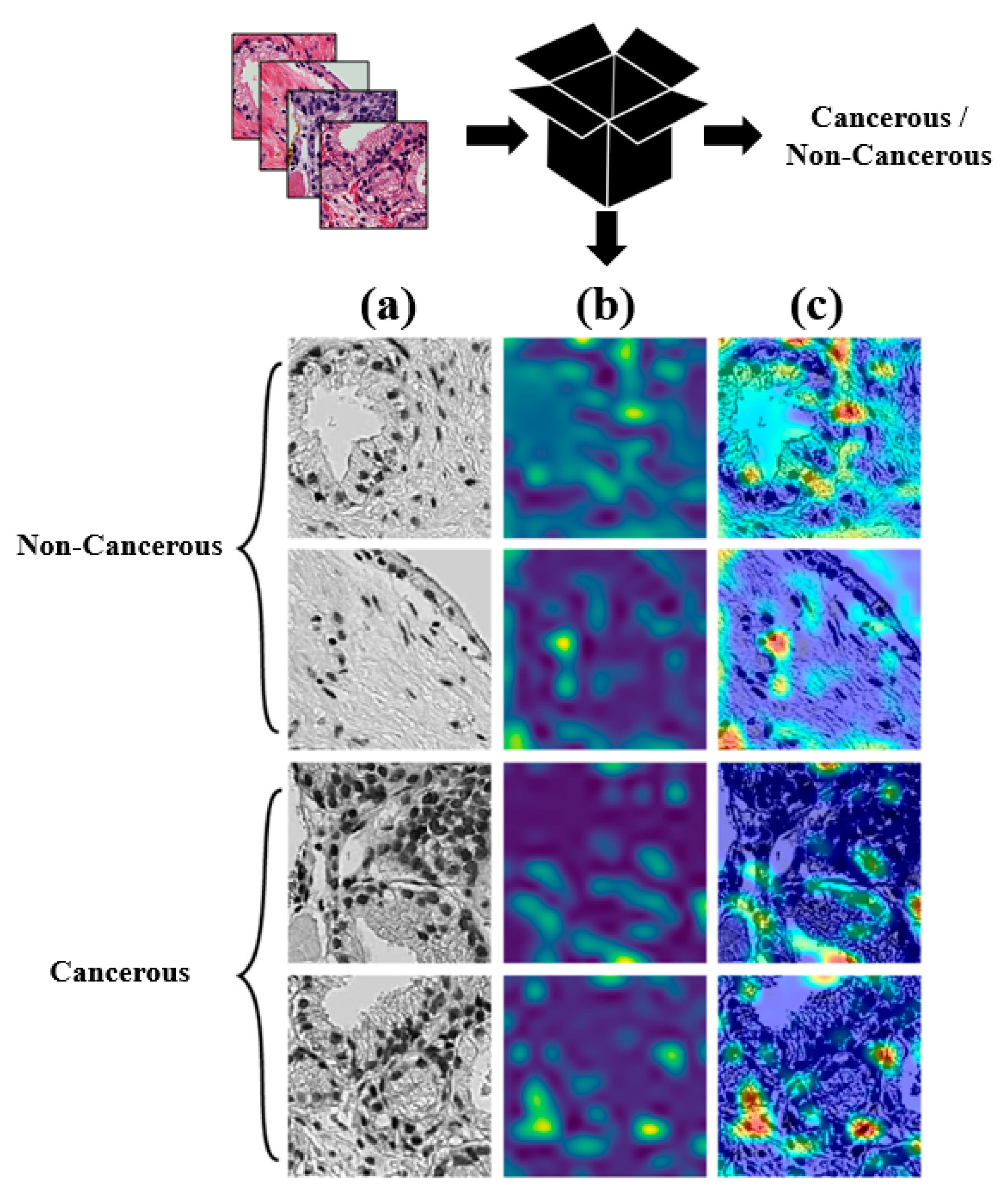
The CAM technique was used to visualize the results from an activation layer (softmax) of the classification block. CAM is used to deduce which regions of an image are used by a CNN to recognize the precise class or group it contains [22,64]. Typically, it is difficult to visualize the results from hidden layers of a black box CNN model. More complexity is observed in feature maps with increasing depth in the network; thus, each image becomes increasingly abstract, encoding less information than the initial layers and appearing more blurred. Figure 11 shows the CAM results, indicating the method by which our DL network detected important regions; moreover, the network had learned a built-in mechanism to determine which regions merited attention. Therefore, this decision process was extremely useful in the classification network.
Our CNN detected specific regions using the softmax classifier by incorporating spatially averaged information extracted by the GAP layer from the last convolution layer, which had an output shape of 14 × 14 × 384. The detected regions depicted in Figure 11c were generated by the application of a heat map to the CAM image in Figure 11b and overlaying that on the original image from Figure 11a. A heat map is highly effective for tissue image analysis; in this instance, it showed how the CNN detected each region of the image that is important for cancer classification. Doctors can use this information to better understand the classification (i.e., how the neural network predicted the presence of cancer in an image, based on the relevant regions). The visualization process was carried out using the test dataset, which was fed into the trained network of model 2.
In this study, supervised classification was performed for cancer grading, whereby our dataset was labeled with “0” and “1” to categorize benign and malignant tissue separately and independently. The probability distributions of data were similar in training and test sets, but the test dataset was independent of the training dataset. Therefore, after the model had been trained with several binary labeled cancer images, the unanalyzed dataset was fed to the network for accurate prediction between binary classes. Figure 12 shows examples of the binary classification results from our proposed model 2, with examples of images that were and were not predicted correctly. Notably, some images of benign were similar to malignant tissues and vice versa in terms of their nuclei distribution, intensity variation, and tissue texture. It was challenging for the model to correctly classify these images into the two groups.

6. Discussion

The main aim of this study was to develop LWCNN for benign and malignant tissue image classification based on multilevel feature map analysis and show the effectiveness of the model. Moreover, we developed an EML voting method for the classification of non-handcrafted (extracted from the GAP layer of model 2) and handcrafted (extracted using OCLBP and IOCLBP). Generally, in DL, the features are extracted automatically from raw data and further processed for classification using a neural network approach. However, for ML algorithms, features are extracted manually using different mathematical formulae; these are also regarded as handcrafted features. A CNN is suitable for complex detection tasks, such as analyses of scattered and finely drawn patterns in data. Of particular interest, in the malignant and benign classification task, model 2 was more effective than model 1.Indeed, model 1 performed below expectation, such that we modified it to improve performance, resulting in model 2. The modification comprised removal of the fourth convolutional block, flattening layer, and sigmoid activation function, as well as alterations of filter number and kernel size. Moreover, GAP replaced flattening after the third convolutional block, minimizing overfitting by reducing the total number of parameters in the model. The softmax activation function replaced the sigmoid activation function in the third dense layer. These modifications, based on the multilevel feature map analysis, improved the overall accuracy and localization ability of tissue image classification.
Furthermore, in this study, we have also compared our proposed CNN model with the well-known pre-trained models such as VGG-16, ResNet-50, Inception-V3, and DenseNet-121. Among these, DenseNet proved to give the highest accuracy of 95% followed by the Inception V3 with 94.6%. The pre-trained VGG-16 and ResNet-50 achieved 92% and 93%, respectively. Although DenseNet gained the highest accuracy among all the pre-trained models as well as our proposed model 2, it is not quite comparable with the motto of this paper. The ultimate goal of this paper was to develop a light-weighted CNN without a much-complicated structure with minimum possible convolutional layers and achieve better classification performance. Model 2 proved this hypothesis by achieving an overall accuracy of 94%. On the other hand, all the pre-trained models are well trained on a huge dataset (ImageNet) which includes 1000 classes. Therefore, it is evident that the classification of such models will be done accurately without much hassle. Nevertheless, the comparison of computational cost between the proposed LWCNN and other pre-trained models was performed to analyze the memory usage, trainable parameters, and learning (training and testing) time, shown in Table 7. First, according to the comparison Table 7, the number of trainable parameters used in the LWCNN model was reduced by more than 75% as compared to VGG-16, ResNet-50, and Inception-V3, and 2% as compared to DenseNet-121. Second, the memory usage of the proposed model was significantly less when compared to other models. Third, the time taken to train the proposed model was also drastically less. Among the pre-trained models, VGG-16 and ResNet-50 agree with the objective of this work. From Table 5 and Table 7, it is evident that our LWCNN (model 2) is competitive and inexpensive, whereas, the state-of-art models were computationally expensive and achieved comparable results. Therefore, from this perspective, model 2 of our proposed work performed better than VGG-16 and ResNet-50 in terms of accuracy, besides employing a simple architecture.
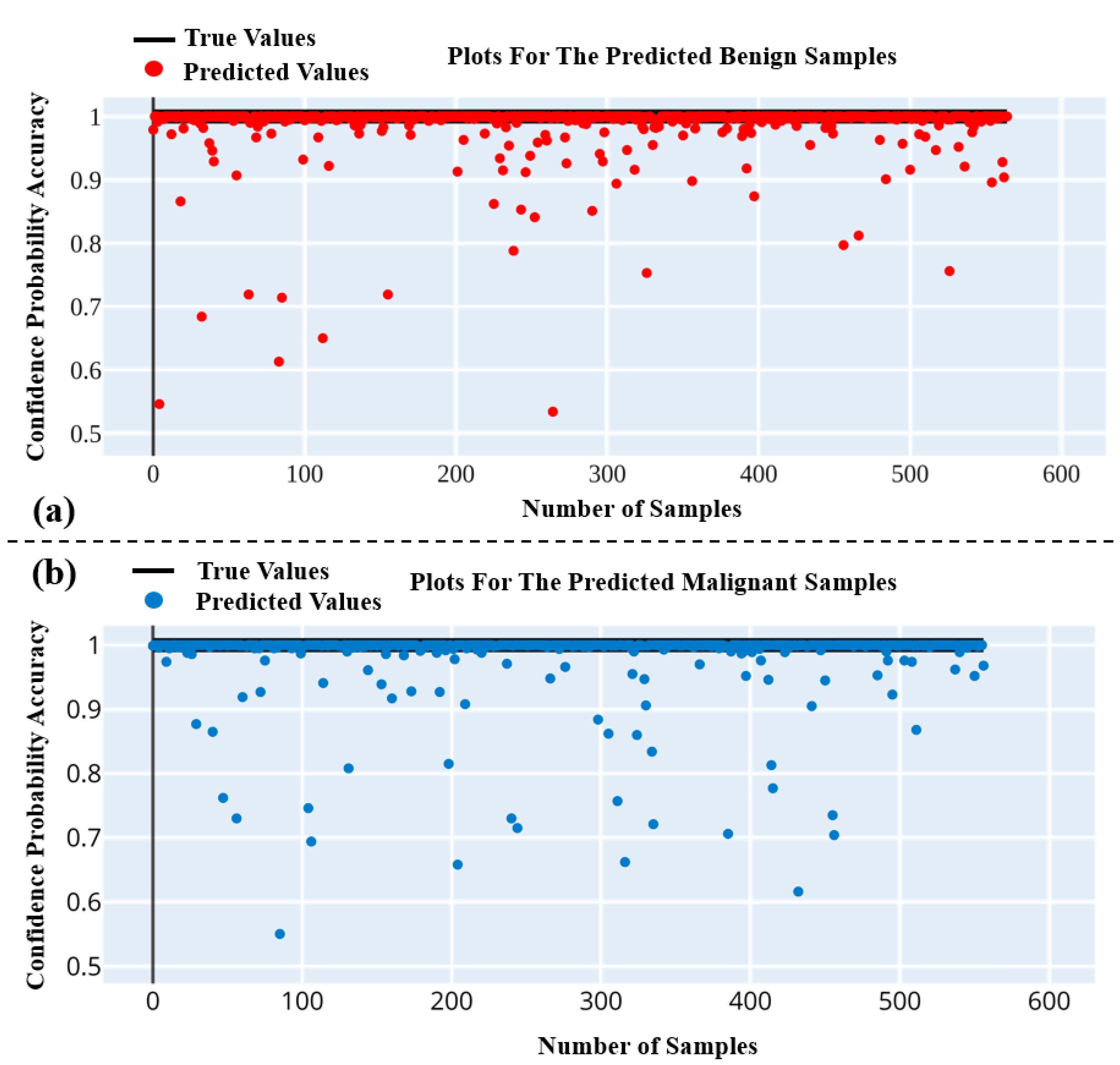
Through fine-tuning of the hyperparameters, the CNN layers were determined to be optimal using the validation and test datasets. The modified, model 2 was adequate for the classification of benign and malignant tissue images. Our study examined the capability of the proposed LWCNN model to detect and forecast the histopathology images; a single activation map was extracted from each block (see Figure 13) to visualize the detection results using a heat map. Notably, we used an EML method for non-handcrafted and handcrafted features classification. However, the EML model was sufficiently powerful to classify the computational features extracted using the optimal LWCNN model, which predicted the samples of benign and malignant tissues almost perfectly accurately. Also, tissue samples that were classified and predicted using the softmax classifier are shown in quantile-quantile (Q−Q) plots of the prediction probability confidence for benign and malignant states in Figure 14a,b, respectively. These Q−Q plots allowed for the analysis of predictions. True and predicted probabilistic values were plotted according to true positive and true negative classifications of samples (see Figure 9), respectively.
In Q−Q plots, note that the black bar at the top parallel to the x-axis shows true probabilistic values; red (true positive) and blue (true negative) markers show the prediction confidence of each sample of a specific class. We used a softmax classifier, which normalizes the output of each unit to be between 0 and 1, ensuring that the probabilities always sum to 1. The number of samples used for each class was 600; the numbers correctly classified were 565 and 557 for true positive and true negative, respectively. A predicted probability value > 0.5 and <0.5 signifies an accurate classification and misclassification, respectively.
The combination of image-feature engineering and ML classification has shown remarkable performance in terms of medical image analysis and classification. In contrast, CNN adaptively learns various image features to perform image transformation, focusing on features that are highly predictive for a specific learning objective [65]. For instance, images of benign and malignant tissues could be presented to a network composed of convolutional layers with different numbers of filters that detect computational features and highlight the pixel pattern in each image. Based on these patterns, the network could use sigmoid and softmax classifiers to learn the extracted and important features, respectively. In DL, the “pipeline” of CNN’s processing (i.e., from inputs to any output prediction) is opaque [66], performed automatically like a passage through a “black box” tunnel, where the user remains fully unaware of the process details. It is difficult to examine a CNN layer-by-layer. Therefore, each layer’s visualization results and prediction mechanism are challenging to interpret.
Overall, all models performed well in tissue image classification, achieving comparable results. The EML method also worked well with CNN-extracted features, yielding comparable results. We conclude that, for image classification, models with very deep layers performed well by more accurately classifying the data samples. We aimed to build an LWCNN model with few feature-map layers and hyperparameters for prediction of cancer grading based on binary classification (i.e., benign vs. malignant). Our proposed methods have proven that lightweight models can achieve good results if the parameters are tuned appropriately. Furthermore, model 2 effectively recognized the histologic differences in tissue images and predicted their statuses with nearly perfect accuracy. The application of DL to histopathology is relatively new. However, it performs well and delivers accurate results. DL methods provide outstanding performance through black box layers; the outputs of each of these layers can be visualized using a heat map. In this study, our model provided insights into the histologic patterns present in each tissue image and can thus assist pathologists as a practical tool for analyzing tissue regions relevant to the worst prognosis. Heat map analyses suggested that the LWCNN can learn visual patterns of histopathological images containing different features relating to nuclear morphology, cell density, gland formation, and variations in the intensity of stroma and cytoplasm. Performance significantly improved when the first model was modified based on the feature map analysis.

7. Conclusions

In this study, 2D image classification was performed using PCa samples by leveraging non-handcrafted and handcrafted texture features to distinguish a malignant state of tissue from a benign state. We have presented LWCNN- and EML-based image and feature classification using feature map analysis. The DL models were designed with only a few CNN layers and trained with a small number of parameters. The computed feature maps of each layer were fed into these fully CNNs through the flattening and GAP layers, enabling binary classification using sigmoid and softmax classifiers. GAP and softmax were used for model 2, the optimal network in this paper. The GAP layer was used, instead of flattening, to minimize overfitting by reducing the total number of parameters in the model. This layer computes the mean value for each feature map, whereas flattening combined all feature maps extracted from the final convolution or pooling layers by changing the shape of the data from a 2D matrix of features into a one-dimensional array for passage to the fully CNN classifier. A comparative analysis was performed between the DL and EML classification results. Moreover, the computational cost was also compared among the models. The optimum LWCNN (i.e., model 2) and EML models (a combination of LR and RF classifiers) achieved nearly perfectly accurate results with significantly fewer trainable parameters. The proposed LWCNN model developed in the study achieved an overall accuracy of 94%, average precision of 94.2%, an average recall of 92.9%, an average f1-score of 93.5%, and MCC of 87%. On the other hand, using CNN-based features, the EML model achieved an overall accuracy of 92%, an average precision of 92.7%, an average recall of 91%, an average f1-score of 91.8%, and MCC of 83.5%.
To conclude, the analysis presented in this study is very encouraging. However, a model built for medical images may not work well for other types of images. There is a need to fine-tune the hyperparameters to control model overfitting and loss, thereby improving accuracy. The 2D LWCNN (model 2) developed in this study performed well, and therefore, the predicted true positive and true negative samples for benign and malignant, respectively, were plotted using Q-Q plots. The CAM technique was used to visualize the results of the block box CNN model. In the future, we will consider other methods and develop a more complex DL model and compare it with our optimal LWCNN model and other transfer learning models. Further, we will extend the research to multi-class classification (beyond binary) to simultaneously classify benign tissues, as well as grades 3–5.

Author Contributions

Funding acquisition, H.-K.C.; Methodology, S.B.; Resources, N.-H.C.; Supervision, H.-K.C.; Validation, H.-G.P.; Visualization, C.-H.K.; Writing—original draft, S.B.; Writing—review and editing, C.-H.K. and D.P. All authors have read and agreed to the published version of the manuscript.

Funding

This research was financially supported by the Ministry of Trade, Industry, and Energy (MOTIE), Korea, under the “Regional Specialized Industry Development Program (R&D, P0002072)” supervised by the Korea Institute for Advancement of Technology (KIAT).

Ethical Approval

All subjects’ written informed consent waived for their participation in the study, which was approved by the Institutional Ethics Committee at College of Medicine, Yonsei University, Korea (IRB no. 1-2018-0044).

Conflicts of Interest

The authors declare that they have no conflicts of interest.

References

  1. Siegel, R.L.; Miller, K.D.; Jemal, A. Cancer statistics, 2015. CA Cancer J. Clin. 2015, 65, 5–29. [Google Scholar] [CrossRef]
  2. Chung, M.S.; Shim, M.; Cho, J.S.; Bang, W.; Kim, S.I.; Cho, S.Y.; Rha, K.H.; Hong, S.J.; Hong, C.-H.; Lee, K.S.; et al. Pathological Characteristics of Prostate Cancer in Men Aged <50 Years Treated with Radical Prostatectomy: A Multi-Centre Study in Korea. J. Korean Med. Sci. 2019, 34, 78. [Google Scholar] [CrossRef]
  3. Yoo, S.; Gujrathi, I.; Haider, M.A.; Khalvati, F. Prostate Cancer Detection using Deep Convolutional Neural Networks. Sci. Rep. 2019, 9, 19518. [Google Scholar] [CrossRef] [Green Version]
  4. Humphrey, P.A. Diagnosis of adenocarcinoma in prostate needle biopsy tissue. J. Clin. Pathol. 2007, 60, 35–42. [Google Scholar] [CrossRef]
  5. Van Der Kwast, T.H.; Lopes, C.; Santonja, C.; Pihl, C.-G.; Neetens, I.; Martikainen, P.; Di Lollo, S.; Bubendorf, L.; Hoedemaeker, R.F. Guidelines for processing and reporting of prostatic needle biopsies. J. Clin. Pathol. 2003, 56, 336–340. [Google Scholar] [CrossRef] [PubMed] [Green Version]
  6. Kim, E.H.; Andriole, G.L. Improved biopsy efficiency with MR/ultrasound fusion-guided prostate biopsy. J. Natl. Cancer Inst. 2016, 108. [Google Scholar] [CrossRef] [PubMed]
  7. Heidenreich, A.; Bastian, P.J.; Bellmunt, J.; Bolla, M.; Joniau, S.; Van Der Kwast, T.; Mason, M.; Matveev, V.; Wiegel, T.; Zattoni, F.; et al. EAU Guidelines on Prostate Cancer. Part 1: Screening, Diagnosis, and Local Treatment with Curative Intent—Update 2013. Eur. Urol. 2014, 65, 124–137. [Google Scholar] [CrossRef] [PubMed]
  8. Humphrey, P.A. Gleason grading and prognostic factors in carcinoma of the prostate. Mod. Pathol. 2004, 17, 292–306. [Google Scholar] [CrossRef]
  9. Nagpal, K.; Foote, D.; Liu, Y.; Chen, P.-H.C.; Wulczyn, E.; Tan, F.; Olson, N.; Smith, M.C.; Mohtashamian, A.; Wren, J.H.; et al. Development and validation of a deep learning algorithm for improving Gleason scoring of prostate cancer. NPJ Digit. Med. 2019, 2, 48. [Google Scholar] [CrossRef] [Green Version]
  10. Alqahtani, S.; Wei, C.; Zhang, Y.; Szewczyk-Bieda, M.; Wilson, J.; Huang, Z.; Nabi, G. Prediction of prostate cancer Gleason score upgrading from biopsy to radical prostatectomy using pre-biopsy multiparametric MRI PIRADS scoring system. Sci. Rep. 2020, 10, 7722. [Google Scholar] [CrossRef]
  11. Zhu, Y.; Freedland, S.J.; Ye, D. Prostate Cancer and Prostatic Diseases Best of Asia, 2019: Challenges and opportunities. Prostate Cancer Prostatic Dis. 2019, 23, 197–198. [Google Scholar] [CrossRef] [PubMed]
  12. Kumar, R.; Srivastava, R.; Srivastava, S.K. Detection and Classification of Cancer from Microscopic Biopsy Images Using Clinically Significant and Biologically Interpretable Features. J. Med. Eng. 2015, 2015, 457906. [Google Scholar] [CrossRef] [PubMed]
  13. Cahill, L.C.; Fujimoto, J.G.; Giacomelli, M.G.; Yoshitake, T.; Wu, Y.; Lin, D.I.; Ye, H.; Carrasco-Zevallos, O.M.; Wagner, A.A.; Rosen, S. Comparing histologic evaluation of prostate tissue using nonlinear microscopy and paraffin H&E: A pilot study. Mod. Pathol. 2019, 32, 1158–1167. [Google Scholar] [CrossRef]
  14. Otali, D.; Fredenburgh, J.; Oelschlager, D.K.; Grizzle, W.E. A standard tissue as a control for histochemical and immunohistochemical staining. Biotech. Histochem. 2016, 91, 309–326. [Google Scholar] [CrossRef] [PubMed] [Green Version]
  15. Alturkistani, H.A.; Tashkandi, F.M.; Mohammedsaleh, Z.M. Histological Stains: A Literature Review and Case Study. Glob. J. Health Sci. 2015, 8, 72. [Google Scholar] [CrossRef] [PubMed]
  16. Zarella, M.D.; Yeoh, C.; Breen, D.E.; Garcia, F.U. An alternative reference space for H&E color normalization. PLoS ONE 2017, 12, 0174489. [Google Scholar]
  17. Lahiani, A.; Klaiman, E.; Grimm, O. Enabling histopathological annotations on immunofluorescent images through virtualization of hematoxylin and eosin. J. Pathol. Inform. 2018, 9, 1. [Google Scholar] [CrossRef] [PubMed]
  18. Gavrilovic, M.; Azar, J.C.; Lindblad, J.; Wählby, C.; Bengtsson, E.; Busch, C.; Carlbom, I.B. Blind Color Decomposition of Histological Images. IEEE Trans. Med. Imaging 2013, 32, 983–994. [Google Scholar] [CrossRef]
  19. Bautista, P.A.; Yagi, Y. Staining Correction in Digital Pathology by Utilizing a Dye Amount Table. J. Digit. Imaging 2015, 28, 283–294. [Google Scholar] [CrossRef]
  20. Bianconi, F.; Kather, J.N.; Reyes-Aldasoro, C.C. Evaluation of Colour Pre-Processing on Patch-Based Classification of H&E-Stained Images. In Digital Pathology. ECDP; Lecture Notes in Computer Science; Springer: Cham, Switzerland, 2019; Volume 11435, pp. 56–64. [Google Scholar] [CrossRef] [Green Version]
  21. Diamant, A.; Chatterjee, A.; Vallières, M.; Shenouda, G.; Seuntjens, J. Deep learning in head & neck cancer outcome prediction. Sci. Rep. 2019, 9, 2764. [Google Scholar]
  22. Yamashita, R.; Nishio, M.; Do, R.K.G.; Togashi, K. Convolutional neural networks: An overview and application in radiology. Insights Imaging 2018, 9, 611–629. [Google Scholar] [CrossRef] [PubMed] [Green Version]
  23. Sahiner, B.; Pezeshk, A.; Hadjiiski, L.; Wang, X.; Drukker, K.; Cha, K.H.; Summers, R.M.; Giger, M.L. Deep learning in medical imaging and radiation therapy. Med. Phys. 2019, 46, e1–e36. [Google Scholar] [CrossRef] [PubMed] [Green Version]
  24. Nanni, L.; Ghidoni, S.; Brahnam, S. Handcrafted vs. non-handcrafted features for computer vision classification. Pattern Recognit. 2017, 71, 158–172. [Google Scholar] [CrossRef]
  25. Lundervold, A.S.; Lundervold, A. An overview of deep learning in medical imaging focusing on MRI. Z. Med. Phys. 2019, 29, 102–127. [Google Scholar] [CrossRef] [PubMed]
  26. Lee, J.-G.; Jun, S.; Cho, Y.-W.; Lee, H.; Kim, G.B.; Seo, J.B.; Kim, N. Deep Learning in Medical Imaging: General Overview. Korean J. Radiol. 2017, 18, 570–584. [Google Scholar] [CrossRef] [PubMed] [Green Version]
  27. Bi, W.L.; Hosny, A.; Schabath, M.B.; Giger, M.L.; Birkbak, N.J.; Mehrtash, A.; Allison, T.; Arnaout, O.; Abbosh, C.; Dunn, I.F.; et al. Artificial intelligence in cancer imaging: Clinical challenges and applications. CA Cancer J. Clin. 2019, 69, 127–157. [Google Scholar] [CrossRef] [Green Version]
  28. Jha, S.; Topol, E.J. Adapting to Artificial Intelligence. JAMA 2016, 316, 2353–2354. [Google Scholar] [CrossRef] [PubMed]
  29. Badejo, J.A.; Adetiba, E.; Akinrinmade, A.; Akanle, M.B. Medical Image Classification with Hand-Designed or Machine-Designed Texture Descriptors: A Performance Evaluation. In Internatioanl Conference on Bioinformatics and Biomedical Engineering; Springer: Cham, Switzerland, 2018; pp. 266–275. [Google Scholar] [CrossRef]
  30. Bianconi, F.; Bello-Cerezo, R.; Napoletano, P. Improved opponent color local binary patterns: An effective local image descriptor for color texture classification. J. Electron. Imaging 2017, 27, 011002. [Google Scholar] [CrossRef]
  31. Kather, J.N.; Bello-Cerezo, R.; Di Maria, F.; Van Pelt, G.W.; Mesker, W.E.; Halama, N.; Bianconi, F. Classification of Tissue Regions in Histopathological Images: Comparison Between Pre-Trained Convolutional Neural Networks and Local Binary Patterns Variants. In Intelligent Systems Reference Library; Springer: Cham, Switzerland, 2020; pp. 95–115. [Google Scholar] [CrossRef]
  32. Khairunnahar, L.; Hasib, M.A.; Bin Rezanur, R.H.; Islam, M.R.; Hosain, K. Classification of malignant and benign tissue with logistic regression. Inform. Med. Unlocked 2019, 16, 100189. [Google Scholar] [CrossRef]
  33. Guidotti, R.; Monreale, A.; Ruggieri, S.; Turini, F.; Giannotti, F.; Pedreschi, D. A Survey of Methods for Explaining Black Box Models. ACM Comput. Surv. 2019, 51, 93. [Google Scholar] [CrossRef] [Green Version]
  34. Hayashi, Y. New unified insights on deep learning in radiological and pathological images: Beyond quantitative performances to qualitative interpretation. Inform. Med. Unlocked 2020, 19, 100329. [Google Scholar] [CrossRef]
  35. Lo, S.-C.; Lou, S.-L.; Lin, J.-S.; Freedman, M.; Chien, M.; Mun, S. Artificial convolution neural network techniques and applications for lung nodule detection. IEEE Trans. Med. Imaging 1995, 14, 711–718. [Google Scholar] [CrossRef] [PubMed]
  36. Lo, S.-C.B.; Chan, H.-P.; Lin, J.-S.; Li, H.; Freedman, M.T.; Mun, S.K. Artificial convolution neural network for medical image pattern recognition. Neural Netw. 1995, 8, 1201–1214. [Google Scholar] [CrossRef]
  37. LeCun, Y.; Bottou, L.; Bengio, Y.; Haffner, P. Gradient-based learning applied to document recognition. Proc. IEEE 1998, 86, 2278–2324. [Google Scholar] [CrossRef] [Green Version]
  38. Liu, S.; Zheng, H.; Feng, Y.; Li, W. Prostate cancer diagnosis using deep learning with 3D multiparametric MRI. In Medical Imaging 2017: Computer-Aided Diagnosis; SPIE 10134; International Society for Optics and Photonics: Orlando, FL, USA, 2017; p. 1013428. [Google Scholar]
  39. Han, Z.; Wei, B.; Zheng, Y.; Yin, Y.; Li, K.; Li, S. Breast Cancer Multi-classification from Histopathological Images with Structured Deep Learning Model. Sci. Rep. 2017, 7, 4172. [Google Scholar] [CrossRef]
  40. Abraham, B.; Nair, M.S. Automated grading of prostate cancer using convolutional neural network and ordinal class classifier. Inform. Med. Unlocked 2019, 17, 100256. [Google Scholar] [CrossRef]
  41. Truki, T. An Empirical Study of Machine Learning Algorithms for Cancer Identification. In Proceedings of the 2018 IEEE 15th International Conference on Networking, Sensing and Control (ICNSC), Zhuhai, China, 27–29 March 2018; pp. 1–5. [Google Scholar]
  42. Veta, M.M.; Pluim, J.P.W.; Van Diest, P.J.; Viergever, M.A. Breast Cancer Histopathology Image Analysis: A Review. IEEE Trans. Biomed. Eng. 2014, 61, 1400–1411. [Google Scholar] [CrossRef]
  43. Moradi, M.; Mousavi, P.; Abolmaesumi, P. Computer-Aided Diagnosis of Prostate Cancer with Emphasis on Ultrasound-Based Approaches: A Review. Ultrasound Med. Biol. 2007, 33, 1010–1028. [Google Scholar] [CrossRef]
  44. Alom, Z.; Yakopcic, C.; Nasrin, M.S.; Taha, T.M.; Asari, V.K. Breast Cancer Classification from Histopathological Images with Inception Recurrent Residual Convolutional Neural Network. J. Digit. Imaging 2019, 32, 605–617. [Google Scholar] [CrossRef] [Green Version]
  45. Wang, C.; Shi, J.; Zhang, Q.; Ying, S. Histopathological image classification with bilinear convolutional neural networks. In Proceedings of the 2017 39th Annual International Conference of the IEEE Engineering in Medicine and Biology Society (EMBC), Seogwipo, Korea, 15–16 July 2017; Volume 2017, pp. 4050–4053. [Google Scholar]
  46. Smith, S.A.; Newman, S.J.; Coleman, M.P.; Alex, C. Characterization of the histologic appearance of normal gill tissue using special staining techniques. J. Vet. Diagn. Investig. 2018, 30, 688–698. [Google Scholar] [CrossRef] [Green Version]
  47. Vodyanoy, V.; Pustovyy, O.; Globa, L.; Sorokulova, I. Primo-Vascular System as Presented by Bong Han Kim. Evid. Based Complement. Altern. Med. 2015, 2015, 361974. [Google Scholar] [CrossRef] [PubMed] [Green Version]
  48. Larson, K.; Ho, H.H.; Anumolu, P.L.; Chen, M.T. Hematoxylin and Eosin Tissue Stain in Mohs Micrographic Surgery: A Review. Dermatol. Surg. 2011, 37, 1089–1099. [Google Scholar] [CrossRef] [PubMed]
  49. Huang, S.-C.; Cheng, F.-C.; Chiu, Y.-S. Efficient Contrast Enhancement Using Adaptive Gamma Correction With Weighting Distribution. IEEE Trans. Image Process. 2012, 22, 1032–1041. [Google Scholar] [CrossRef] [PubMed]
  50. Rahman, S.; Rahman, M.; Abdullah-Al-Wadud, M.; Al-Quaderi, G.D.; Shoyaib, M. An adaptive gamma correction for image enhancement. EURASIP J. Image Video Process. 2016, 2016, 35. [Google Scholar] [CrossRef] [Green Version]
  51. Shorten, C.; Khoshgoftaar, T.M. A survey on Image Data Augmentation for Deep Learning. J. Big Data 2019, 6, 60. [Google Scholar] [CrossRef]
  52. Lecun, Y.; Bengio, Y.; Hinton, G. Deep learning. Nature 2015, 521, 436–444. [Google Scholar] [CrossRef]
  53. Kieffer, B.; Babaie, M.; Kalra, S.; Tizhoosh, H.R. Convolutional neural networks for histopathology image classification: Training vs. Using pre-trained networks. In Proceedings of the 2017 Seventh International Conference on Image Processing Theory, Tools and Applications (IPTA), Montreal, QC, Canada, 28 November–1 December 2017; pp. 1–6. [Google Scholar]
  54. Mourgias-Alexandris, G.; Tsakyridis, A.; Passalis, N.; Tefas, A.; Vyrsokinos, K.; Pleros, N. An all-optical neuron with sigmoid activation function. Opt. Express 2019, 27, 9620–9630. [Google Scholar] [CrossRef]
  55. Elfwing, S.; Uchibe, E.; Doya, K. Sigmoid-weighted linear units for neural network function approximation in reinforcement learning. Neural Netw. 2018, 107, 3–11. [Google Scholar] [CrossRef]
  56. Kouretas, I.; Paliouras, V. Simplified Hardware Implementation of the Softmax Activation Function. In Proceedings of the 2019 8th International Conference on Modern Circuits and Systems Technologies (MOCAST), Thessaloniki, Greece, 13–15 May 2019; pp. 1–4. [Google Scholar]
  57. Zhu, Q.; He, Z.; Zhang, T.; Cui, W. Improving Classification Performance of Softmax Loss Function Based on Scalable Batch-Normalization. Appl. Sci. 2020, 10, 2950. [Google Scholar] [CrossRef]
  58. Dietterich, T.G. Ensemble Methods in Machine Learning. In International Workshop on Multiple Classifier System; Springer: Berlin, Heidelberg, 2000; pp. 1–15. [Google Scholar] [CrossRef] [Green Version]
  59. Dikaios, N.; Alkalbani, J.; Sidhu, H.S.; Fujiwara, T.; Abd-Alazeez, M.; Kirkham, A.; Allen, C.; Ahmed, H.; Emberton, M.; Freeman, A.; et al. Logistic regression model for diagnosis of transition zone prostate cancer on multi-parametric MRI. Eur. Radiol. 2015, 25, 523–532. [Google Scholar] [CrossRef] [Green Version]
  60. Nguyen, C.; Wang, Y.; Nguyen, H.N. Random forest classifier combined with feature selection for breast cancer diagnosis and prognostic. J. Biomed. Sci. Eng. 2013, 6, 551–560. [Google Scholar] [CrossRef]
  61. Cruz, J.A.; Wishart, D.S. Applications of Machine Learning in Cancer Prediction and Prognosis. Cancer Inform. 2006, 2, 59–77. [Google Scholar] [CrossRef]
  62. Tang, T.T.; Zawaski, J.A.; Francis, K.N.; Qutub, A.A.; Gaber, M.W. Image-based Classification of Tumor Type and Growth Rate using Machine Learning: A preclinical study. Sci. Rep. 2019, 9, 12529. [Google Scholar] [CrossRef] [PubMed] [Green Version]
  63. Madabhushi, A.; Lee, G. Image analysis and machine learning in digital pathology: Challenges and opportunities. Med. Image Anal. 2016, 33, 170–175. [Google Scholar] [CrossRef] [PubMed] [Green Version]
  64. Yang, W.; Huang, H.; Zhang, Z.; Chen, X.; Huang, K.; Zhang, S. Towards Rich Feature Discovery With Class Activation Maps Augmentation for Person Re-Identification. In Proceedings of the 2019 IEEE/CVF Conference on Computer Vision and Pattern Recognition (CVPR), Long Beach, CA, USA, 15–20 June 2019; pp. 1389–1398. [Google Scholar]
  65. Hou, X.; Gong, Y.; Liu, B.; Sun, K.; Liu, J.; Xu, B.; Duan, J.; Qiu, G. Learning Based Image Transformation Using Convolutional Neural Networks. IEEE Access 2018, 6, 49779–49792. [Google Scholar] [CrossRef]
  66. Chai, X.; Gu, H.; Li, F.; Duan, H.; Hu, X.; Lin, K. Deep learning for irregularly and regularly missing data reconstruction. Sci. Rep. 2020, 10, 3302. [Google Scholar] [CrossRef]
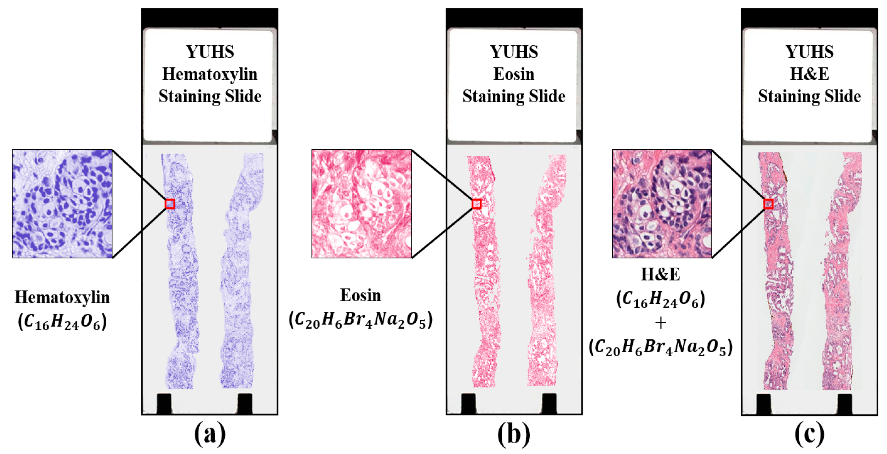
Figure 1. The visualization result of hematoxylin and eosin (H&E) staining slide. (a) Hematoxylin staining slide. (b) Eosin staining slide. (c) H&E staining slide obtained by combining (a,b). Note that the two slides (a,b) are highly dissimilar in texture, which is useful for analysis and classification.
Applsci 10 08013 g001
Figure 2. Data preparation of a sample histopathology slide from a prostatectomy. (a) An example of a whole-slide image where a sliding window method was applied to generate patch images. (b) The cropped patches obtained from (a) corresponded to the lowest and highest Gleason pattern, from well-differentiated to poorly differentiated, respectively. Among all patches in (b), the simple stroma, benign and malignant patches were selected for PCa analysis and classification.
Applsci 10 08013 g002
Figure 3. Proposed pipeline for image and feature classification based on a lightweight convolutional neural network (LWCNN) and ensemble machine learning (EML). LR: logistic regression, RF: random forest.
Applsci 10 08013 g003
Figure 4. Image preprocessing using smoothing and gamma correction. (a,c) Original images of benign and malignant tissues, respectively. Here, the images are blurry and exhibit low contrast. (b,d) Images after removal of random noise, smoothing, and gamma correction. (e) Transformation curve for images with low and high contrast. Because the images in (a,c) have low contrast, γ = 2 was applied to adjust their intensities, obtaining images in (b,d) that appear clear and “fresh.” Therefore, the tissue components were more visible after transformation, which was important for CNN classification.
Applsci 10 08013 g004
Figure 5. Randomly selected samples from the training dataset demonstrating data augmentation. (a,b) Images of benign and malignant tissues, respectively, before the transformation. (c,d) Transformed images from (a,b), respectively, after data augmentation.
Applsci 10 08013 g005
Figure 6. Structure of our lightweight convolutional neural networks for cancer image classification between two Gleason grade groups of prostate carcinoma. Spatial features are extracted from an image by convolving through one of the networks. Classification layers (flatten, global average pooling [GAP], dense-1, dense-2, and output) were used to find the required response based on features that were extracted by the convolutional neural network.
Applsci 10 08013 g006
Figure 7. Multilevel feature map analysis for tissue image classification using a lightweight convolutional neural network. Visual analysis was performed by observing the pixel pattern in feature maps extracted from each block. Each block holds different information that is useful for convolutional neural network classification. Output shapes of feature maps from blocks 1−4 were: 56 × 56 × 92, 28 × 28 × 192, 14 × 14 × 384, and 7 × 7 × 512, respectively. Shown are four feature maps per block for the purpose of analysis, with 92, 192, 384, and 512 in each block, respectively. Analysis reveals that block-4 contains the maximum information regarding the image, but the resulting maps are less visually interpretable by people. With advancement deeper into the network, the feature maps become sparser, indicating that convolution filters detect fewer features. Therefore, block-4 was removed from model 2.
Applsci 10 08013 g007
Figure 8. Flow diagram for DL and ML classification. Handcrafted and non-handcrafted colour texture descriptors were extracted for EML classification.
Applsci 10 08013 g008
Figure 9. ROC curves for analyzing the behavior of different optimizers, generated by plotting predicted probability values (i.e., model’s confidence scores). (a) Performance of model 1 based on sigmoid activation. (b) Performance of model 2 based on softmax activation function.
Applsci 10 08013 g009
Figure 10. Confusion matrix of model 2, generated using the test dataset, showing results of binary classifications between benign (0) and malignant (1) tumors. Blue boxes at top-left and bottom-right represent true positive and true negative, respectively; white boxes at top-right and bottom-left represent false negative and false positive, respectively.
Applsci 10 08013 g010
Figure 11. Class activation maps are extracted from one of the classification layers of our convolutional neural network. These show how images are classified and predicted by the neural network, although it is a black-box model. Top and bottom pairs of rows depict benign and malignant tissue images, respectively. (a) Input images with an RGB color scheme visualized as grayscale. (b) Activation map of classification block, showing detection of different regions in each tissue image. (c) Images overlaying (a,b), with spots indicating significant regions that the convolutional neural network used to identify a specific in that image.
Applsci 10 08013 g011
Figure 12. Cancer prediction using a binary labeled test dataset. Examples of images that were (a) correctly and (b) incorrectly classified, showing their actual and predicted labels.
Applsci 10 08013 g012
Figure 13. Visualizations of class activation maps generated from model 2, created using different numbers of filters. Outputs of (a) first convolutional, (b) second convolutional, (c) third convolutional, and (d) classification blocks. Colors indicate the most relevant regions for predicting the class of these histopathology images, as detected by the convolutional neural network.
Applsci 10 08013 g013
Figure 14. Quantile-quantile plot for true and predicted probabilistic values. (a) Samples that were benign and had true positive predictions. (b) Samples that were malignant and had true negative predictions.
Applsci 10 08013 g014
Table 1. Assignment of benign and malignant samples into datasets for training, validation, and testing.
DatasetBenign (0)Malignant (1)Total
Training180018003600
Validation6006001200
Testing6006001200
Total300030006000
Table 2. Detailed information and specifications of lightweight convolutional neural network models. BN: batch normalization, GAP: global average pooling, ReLU: rectified linear unit.
Layer TypeFiltersOutput ShapeKernel Size/Strides
Model-1 Specification
InputImage1224 × 224 × 3-
Block-12× convolutional + ReLU + BN3256 × 56 × 323 × 3/2
Block-22× convolutional + ReLU + BN6456 × 56 × 643 × 3/1
-Max pooling + dropout (0.25)6428 × 28 × 642 × 2/2
Block-33× convolutional + ReLU + BN12828 × 28 × 1283 × 3/1
-Max pooling + dropout (0.25)12814 × 14 × 1282 × 2/2
Block-43× convolutional + ReLU + BN25614 × 14 × 2563 × 3/1
-Max pooling + dropout (0.25)2567 × 7 × 2562 × 2/2
-Flatten-12,544-
-Dense-1 + ReLU + BN10241024-
-Dense-2 + ReLU + BN10241024-
-Dropout (0.5)10241024-
OutputSigmoid22-
Model-2 specification
InputImage1224 × 224 × 3-
Block-12× convolutional + ReLU + BN9256 × 56 × 925 × 5/2
Block-22× convolutional + ReLU + BN19256 × 56 × 1923 × 3/1
-Max pooling19228 × 28 × 1922 × 2/2
Block-33× convolutional + ReLU + BN38428 × 28 × 3843 × 3/1
-Max pooling + dropout (0.25)38414 × 14 × 3842 × 2/2
-GAP-3842 × 2/2
-Dense-1 + ReLU + BN6464-
-Dense-2 + ReLU + BN3232-
-Dropout (0.5)3232-
OutputSoftmax22-
Table 3. Hyperparameters Tuning for DL and ML classifiers.
ModelsSpecification
Model-1, VGG-16, ResNet-50, Inception-V3, DenseNet-121loss = binary_crossentropy; learning rate = start:1.0—auto reduce on plateau fraction: 0.8 after 10 consecutive non-declines of validation loss; classifier = sigmoid; epochs = 300
Model-2loss = binary_crossentropy; learning rate = start:1.0—auto reduce on plateau fraction: 0.8 after 10 consecutive non-declines of validation loss; classifier = softmax; epochs = 300, kernel initializer = glorot_uniform
LRC = 100, max_iter = 500, tol = 0.001, method = isotonic, penalty = l2
RFn_estimators = 500, criterion = gini, max_depth = 9, min_samples_split = 5, min_samples_leaf = 4, method = isotonic
Table 4. Comparison of the optimizers for tissue image classification.
Model-1Model-2
OptimizersTest Loss
(%)
Test Accuracy
(%)
Test Loss
(%)
Test Accuracy
(%)
SGD0.5185.70.2593.3
RMSProp1.0085.50.6289.3
Adam0.4584.40.2891.1
Adadelta0.5489.10.2594.0
Table 5. Comparative analysis of lightweight and pre-trained CNN models based on non-handcrafted features. Metrics are for the test dataset.
Deep Learning
Model-1Model-2VGG-16ResNet-50Inception-V3DenseNet-121
Accuracy89.1%94.0%92.0%93.0%94.6%95.0%
Precision89.2%94.2%92.2%95.0%96.5%96.2%
Recall89.1%92.9%91.9%90.6%93.2%94.6%
F1-Score89.0%93.5%92.0%92.8%94.8%95.4%
MCC78.3%87.0%84.0%85.3%89.5%90.7%
Table 6. Comparative analysis of non-handcrafted and handcrafted features classification. Metrics are for the test dataset.
Ensemble Machine Learning
CNN-BasedOCLBPIOCLBPOCLBP + IOCLBP
Accuracy92.0%69.3%83.6%85.0%
Precision92.7%66.0%83.2%85.5%
Recall91.0%70.6%83.9%84.5%
F1-Score91.8%68.2%83.5%85.0%
MCC83.5%38.6%67.2%69.8%
Table 7. Comparing performance and computation cost of model-2 with other pre-trained models.
ModelsParameter (Trainable)Model
Memory Usage
Time to Solution (Minutes)
TrainTest
VGG-1627,823,93860.9 MB570<1
ResNet-5023,538,690148.4 MB660<1
Inception-V322,852,89866.9 MB 600 <1
DenseNet-1217,479,682199.7 MB700<1
Model-2 (LWCNN)5,386,63844.7 MB190<1
Publisher’s Note: MDPI stays neutral with regard to jurisdictional claims in published maps and institutional affiliations.