A Novel Assisted Artificial Neural Network Modeling Approach for Improved Accuracy Using Small Datasets: Application in Residual Strength Evaluation of Panels with Multiple Site Damage Cracks

Abstract

An artificial neural network (ANN) extracts knowledge from a training dataset and uses this acquired knowledge to forecast outputs for any new set of inputs. When the input/output relations are complex and highly non-linear, the ANN needs a relatively large training dataset (hundreds of data points) to capture these relations adequately. This paper introduces a novel assisted-ANN modeling approach that enables the development of ANNs using small datasets, while maintaining high prediction accuracy. This approach uses parameters that are obtained using the known input/output relations (partial or full relations). These so called assistance parameters are included as ANN inputs in addition to the traditional direct independent inputs. The proposed assisted approach is applied for predicting the residual strength of panels with multiple site damage (MSD) cracks. Different assistance levels (four levels) and different training dataset sizes (from 75 down to 22 data points) are investigated, and the results are compared to the traditional approach. The results show that the assisted approach helps in achieving high predictions’ accuracy (<3% average error). The relative accuracy improvement is higher (up to 46%) for ANN learning algorithms that give lower prediction accuracy. Also, the relative accuracy improvement becomes more significant (up to 38%) for smaller dataset sizes.

1. Introduction

Data-driven methods are increasingly being used in a wide variety of scientific fields. These methods extract knowledge and insights from datasets, which are typically large, and use this acquired knowledge to forecast new outputs. Artificial neural network (ANN) modeling is one of these data-driven methods that resembles the work principle of the human brain. An ANN acquires knowledge through a learning process and stores this knowledge through interneuron connections of different synaptic weight [1]. The ANN learns how a system behaves based on experience gained from the input/output dataset (the training process), and based on that, it can predict the system’s output(s) for any new set of inputs. The ability of the ANNs to learn by example, makes them particularly useful for modeling highly complicated and non-linear processes, since the development of analytical models for such processes is extremely difficult. ANN modeling has been successfully used in a wide variety of engineering applications including automatic control [2], solar energy systems [3,4], traffic and transportation [5], image processing [6], biomechanics [7], materials science and engineering [8,9,10], manufacturing [11,12], fracture mechanics and fault detection [13,14,15,16,17,18,19,20,21,22,23,24,25,26,27].

A typical ANN consists of an input layer, an output layer and one or more hidden layers in between. Networks with up to two hidden layers are typically referred to as shallow neural networks (SNNs). They are the simplest type of networks and the most widely used in engineering applications. Networks with three or more hidden layers are referred to as deep neural networks (DNNs). They generally have higher prediction accuracy, and nowadays, they are attracting the most interest in the field of machine learning [14]. However, DNNs typically require large datasets for training the network in order to achieve high prediction accuracy for the unseen datasets. For applications where the number of inputs is relatively large, datasets comprising >10⁴ data points are typically required [14]. Collecting and assembling large datasets is challenging, or even not feasible, in many applications, such as fracture mechanics and material science. For this reason, DNNs are still not finding a lot of use in some engineering applications. Most SNNs utilize only one hidden layer, and they generally do not require training datasets as large as those needed for DNNs. But nevertheless, even with a single hidden layer network, datasets comprising hundreds of data points are typically required to successfully train the network in order to achieve high prediction accuracy for the unseen dataset. It can be generally stated that the more complex and non-linear the relationships being modeled by the ANN are, the larger the size of the dataset required for training the network is.

In fracture mechanics, ANNs were mostly used in applications concerned with crack propagation, fatigue life, and failure mode prediction [13]. In the field of mechanical fracture, ANNs have not found as much use as in other fields, mainly because it is not easy to generate large experimental datasets for training the ANN. This can mainly be attributed to practical constraints related to the time and cost requirements in many mechanical fracture experiments. Multiple site damage (MSD) cracks are small fatigue cracks that may accumulate at the sides of highly loaded rivet holes in the fuselage of an airplane. These MSD cracks usually appear after an extended period of time due to the large number of loading cycles, and therefore they present a major concern for aging aircraft fleets. Aircraft manufacturers design the fuselage of their airplanes to be able to carry the design load with the presence of a relatively large crack spanning several adjacent rivet holes. However, the presence of MSD cracks can significantly reduce the structure’s ability to carry loads [28]. The maximum stress level a cracked structure can withstand before it fractures is referred to as residual strength. For a panel having a lead (large) crack along with MSD cracks, residual strength usually refers to the stress level at which the ligaments between the lead crack and adjacent MSD cracks, on both sides, collapse. Several analytical and computational methodologies can theoretically be used to estimate the residual strength of panels with MSD, and the accuracy of these methodologies varies substantially [29,30,31,32,33,34].

The use of data-driven approaches, such as ANN, for predicting residual strength of panels with MSD cracks is very rare in literature. As a matter of fact, testing panels with MSD cracks is not a quick and easy experimental task, and it is usually a time-and-cost-intensive process in both preparation and testing. In general, the panels need to be relatively large in order to resemble the actual case of aircraft structures realistically. For this reason, it is not possible to find large experimental datasets for panels with MSD in the literature. Pidaparti et al. [25,26] used ANN for predicting the corrosion rate and residual strength of unstiffened aluminum panels with corrosion thinning and MSD. Comparison of the ANN residual strength predictions with the experimental results showed that the mean absolute error to be about 12%. Such an error level is considered to be relatively high, even when compared to some of the other relatively simple engineering models reported in the literature [29,30,31,32,33,34]. The reason behind this relatively high ANN prediction error can partly be attributed to the small size of the dataset used for training the network (only about 40 data points). The authors of this study, Hijazi et al. [27], have recently used ANN modeling for residual strength prediction of panels with MSD. A dataset comprising 147 different configurations was assembled form many literature sources where 97 data points were used for training, 25 data points for validation and 25 data points for testing. The dataset included data for three different aluminum alloys (2024-T3, 2524-T3 and 7075-T6), four different test panel configurations (unstiffened, stiffened, stiffened with broken middle stiffener, and lap-joints), and many different panel and cracks geometries. Through the careful selection of the ANN inputs and the use of a comprehensive optimization procedure, a single ANN model was developed where this model was able to give reasonably accurate residual strength predictions for all the different materials and panel configurations. Comparison of the ANN model predictions with the experimental results (of the testing dataset) showed that the mean absolute error is less than 4%, which puts the ANN model at the same accuracy level with the best semi-analytical and computational models available in the literature.

Situations where only small experimental datasets are available may be encountered in many fields because generating large datasets is time-and-cost prohibitive [14,27,35,36]. Therefore, different methods have been developed and implemented in ANN modeling to cope with the small dataset conditions. Examples of these methods include using simulated data [37], using virtual data [38], using multiple runs for models development and surrogate data analysis for model validation [39], using duplicated experimental runs [9], using stacked auto-encoder pre-training [14], using analytical models with errors revised by intelligent algorithms [35], using optimization aided generalized regression approach [36], and simultaneously considering data samples with their posterior probabilities [40]. Candelieri et al. [37] used datasets obtained from finite element simulations to develop an ANN model for diagnosing and predicting cracks in aircraft fuselage panels. The use of simulated data was shown to be technically effective and economical compared to generating an experimental dataset; however, the attainable accuracy of such approach is practically limited by the accuracy of the simulation method used to generate the dataset. Li et al. [38] proposed an approach called “functional virtual population” to assist learning of the scheduling knowledge in dynamic manufacturing systems using small datasets. Using as few as 40 virtual samples, the proposed ANN model was attested to enhance learning accuracy. Shaikhina and Khovanova [39] introduced a method of multiple runs adopted during the design of an ANN model for predicting the compressive strength of trabecular bone. Although a small dataset with only 35 data points is used for training, a two-layer back-propagation neural network (BPNN) model achieved significantly high accuracy with 98.3% correlation coefficient between predicted and experimental values. Altarazi et al. [9] used the results of multiple experimental duplicates for the same input variables in developing an ANN model to evaluate polyvinylchloride composites’ properties. Their results showed that the use of the individual duplicates data (instead of the averaged value) helps in enhancing the accuracy of the ANN model. Feng et al. [14] performed pre-training using a stacked auto-encoder to optimize the initial weights in deep networks. They used this approach for predicting solidification cracking susceptibility of stainless steels using a small dataset (containing 487 data points) and concluded that their approach leads to better performance of DNNs. Wu et al. [35] compared four models for the prediction of the flow stress of Nb-Ti micro-alloyed steel. The compared models included the original Arrhenius-type model and the same model modified by intelligent algorithms such as ANN and genetic algorithm. The results showed that the Arrhenius-type model with errors revised by ANN gives the best prediction accuracy among all other models, even with a small training dataset. Qiao et al. [36] proposed the use of a generalized regression neural network (GRNN) optimized by fruit-fly optimization algorithm (FOA) to improve the predictive accuracy when using small training datasets. Using a small dataset comprising only 14 data points, the proposed approach was used for modeling the relationship between alloying elements and fracture toughness of steel alloys. Based on their results, the GRNN-FOA model was found to be successful in predicting toughness with high accuracy and good generalization ability. Mao et al. [40] utilized support vector machine to obtain posterior probability information, then an ANN model whose inputs included the samples and their posterior probabilities was constructed. Using a small dataset, the inclusion of simulation and real data results showed improved learning accuracy by the proposed algorithm.

In this paper, we introduce a novel assisted-ANN modeling approach and use it for estimating the residual strength of panels with MSD. This proposed approach improves the accuracy of the ANN model predictions, and most importantly, it enables the ANN to be trained using small datasets and still achieve high prediction accuracy. Our approach merges the well-known and well-established analytical relations (between the different input/output parameters) with the ANN technique to improve the ability of ANN to estimate the residual strength of panels with MSD cracks. This proposed approach is especially useful in cases where there are many input parameters that affect the output, and at the same time, the number of data points available for training the ANN model is limited. Our approach relies on calculating characteristic quantities using the known relations between the different inputs/outputs and using these calculated quantities as assistance input parameters for the ANN (in addition to the traditional independent inputs). When the size of the training dataset is small, the limited number of data points along with the complex interactions between the inputs/outputs, limits the ability for the ANN to fully capture (or learn) the complex relations between the inputs/outputs. In such cases, the proposed assisted approach helps to improve the ANN training process and enables the network to capture the inputs/outputs relations more adequately, and thus it improves the predictions’ accuracy. As a matter of fact, the choice of the assistance parameters for any type of problem requires sufficient experience in that particular field, since the assistance parameters are chosen based on the specific knowledge of the existing relations between the inputs and outputs. The experimental dataset used in this investigation is obtained from several literature sources [30,31,32,34,41,42]. The data covers four different panel configurations (unstiffened, stiffened, stiffened with middle broken stiffener, bolted lap-joint), different panel widths, sheet thickness, material conditions and grain orientations, along with many different lead and MSD cracks geometries. The dataset includes a total of 113 data points, each representing a unique experimental configuration. In order to demonstrate the benefit of using the proposed assisted-ANN approach, four different levels of assistance are investigated and compared. In addition to the assisted approach, the traditional approach, which relies on the use of independent geometric/material inputs only, is also used on the same data to serve as a benchmark. In our assisted approach, any known partial or full relation between any of the inputs and the output can be used to generate an assistance parameter. For the MSD problem at hand, the assistance parameters being used are mainly the crack-tip stress intensity factor (SIF) correction factors. These SIF correction factors are mainly geometry and configuration dependent, and hence they relate many of the geometric parameters to the residual strength. In addition to these SIF correction factors, theoretical residual strength predictions obtained using an analytical model (called the “Linkup model”), are also used as one of the assistance input parameters. Comparing the results obtained using the traditional and the assisted approaches shows that the assisted-ANN approach clearly improves the accuracy of the ANN residual strength predictions. Based on the testing dataset, the mean absolute percentage error (MAE_p) went from 3.8% for the traditional approach, down to 2.97% for the assisted approach, which means that the relative error reduction is about 22%. The improvement attained using the assisted approach is clearly observed for all the three different ANN learning algorithms that are used in this study, namely; Bayesian Regularization (BR), Levenberg-Marquardt (LM) and Scaled Conjugate Gradient (SCG). Additionally, in order to further demonstrate the benefit of the proposed assisted-ANN approach for small datasets, the size of the training dataset is reduced from 75 data points (the initial size) all the way down to 22 data points, in three steps. As expected, reducing the size of the training dataset increases the error level for the ANN predictions. However, the results show that the relative error reduction, resulting from using the assisted approach, increases for smaller datasets. Therefore, the importance of using the assisted approach is more apparent for smaller datasets since the relative accuracy improvement becomes more significant. The assisted-ANN approach proposed here should prove to be very helpful in cases where the number of data points available for training the ANN is limited, which is generally the case in many experimental investigations in fracture mechanics. In addition, the use of such approach is not limited to fracture mechanics, but it is also generally applicable in other fields where the known analytical inputs/outputs relations can be used as inputs for assisting the ANN training/prediction process. This approach is especially useful when the number of available data points is not sufficient to enable the ANN to fully capture the existing relations between the different inputs/outputs.

2. Background

2.1. Residual Strength of Panels with MSD

A variety of analytical and computational approaches can theoretically be used for estimating the residual strength of panels with MSD cracks. These approaches include analytical, semi-analytical (empirically corrected), computational and data-driven, and the accuracy of these approaches varies significantly [27]. Figure 1 illustrates the configuration of a typical panel having a lead crack along with adjacent MSD cracks, which is being considered here. Linear Elastic Fracture Mechanics (LEFM) is one of the most fundamental theories in fracture mechanics, and it can be used for evaluating residual strength for different types of crack configurations [43]. However, the LEFM is more applicable to brittle materials since it assumes a linear-elastic behavior for the material at the crack tip. According to LEFM, failure (or unstable crack extension) will occur when the value of the crack-tip SIF reaches a critical value. This limiting value of the SIF is called the fracture toughness (K_C). The fracture toughness is a material property, but for thin sheets, it is also slightly dependent on thickness, grain orientation and crack length. For a panel with a major crack and collinear adjacent MSD cracks subjected to tension, as illustrated in Figure 1, the Mode-I stress intensity factor (K_I) for the lead crack is:

$${\mathrm{K}}_{\mathrm{I}}=\mathsf{\sigma }\sqrt{\mathsf{\pi }a} {\mathsf{\beta }}_{\mathrm{W}} {\mathsf{\beta }}_{a/\ell }$$

(1)

where

• σ: The remote applied stress.
• a: Lead crack half-length.
• β_W: Finite width correction factor.
• β_a/ℓ: Cracks interaction correction factor for the effect of MSD cracks on the lead crack.

Thus, the residual strength (σ_c) of the panel can be found as:

$${\mathsf{\sigma }}_{\mathrm{c}}=\frac{{\mathrm{K}}_{\mathrm{C}}}{\sqrt{\mathsf{\pi }a} {\mathsf{\beta }}_{\mathrm{W}} {\mathsf{\beta }}_{a/\ell }}$$

(2)

Experimental investigations have shown that the LEFM is not able to accurately predict the residual strength of panels with MSD neither for brittle nor ductile materials where it consistently over predicts the strength [29]. Swift [28] introduced an analytical model that is specially formulated for the prediction of the residual strength of panels having MSD cracks. This model is called the “Linkup” model, and it is based on the concept that the ligament between the lead crack and the adjacent MSD crack will fail when the remote stress reaches a level that causes the lead crack-tip plastic zone and the adjacent MSD crack-tip plastic zone to touch each other (i.e., merge together). As the linkup occurs, the entire panel will fail (assuming MSD cracks exist on all subsequent holes and no crack arresting structures are used); therefore the stress causing linkup of the lead and MSD cracks is practically equal to the residual strength of the panel. Therefore, the residual strength of panels with MSD is also sometimes referred to as linkup stress.

The Linkup model estimates the plastic zone size using the Irwin plane-stress plastic zone model. The Irwin model is based on the crack-tip SIF (K_I), and it gives the size (diameter) of plastic zone as:

$${\mathrm{r}}_{\mathrm{p}}=\frac{1}{2\pi }{\left(\frac{{\mathrm{K}}_{\mathrm{I}}}{{\mathsf{\sigma }}_{\mathrm{y}}}\right)}^2$$

(3)

where σ_y is the yield strength of the material. Therefore, according to the linkup model, the remote stress that causes failure of the ligament (i.e., touch of the plastic zones), which is called “linkup” stress (σ_LU), is found as:

$${\mathsf{\sigma }}_{\mathrm{c}}={\mathsf{\sigma }}_{\mathrm{LU}}={\mathsf{\sigma }}_{\mathrm{y}}\sqrt{\frac{2\mathrm{L}}{a {\mathsf{\beta }}_a{}^2+\ell {\mathsf{\beta }}_{\ell }{}^2}}$$

(4)

where

• L: Length of the ligament between the lead crack and MSD crack.
• ℓ: MSD crack half-length.
• β_a: The overall SIF correction factor for the lead crack tip.
• β_ℓ: The overall SIF correction factor for the adjacent MSD crack tip.

For the case of a panel with open holes and no stiffeners (as seen in Figure 1), ${\mathsf{\beta }}_a$ and ${\mathsf{\beta }}_{\ell }$ can be determined as follows:

$${\mathsf{\beta }}_a={\mathsf{\beta }}_{\mathrm{W}} {\mathsf{\beta }}_{a/\ell }$$

(5)

$${\mathsf{\beta }}_{\ell }={\mathsf{\beta }}_{\mathrm{H}} {\mathsf{\beta }}_{\ell /a}$$

(6)

where

• β_H: Correction factor for the effect of the hole.
• β_ℓ/a: The cracks interaction correction factor for the effect of the lead crack on MSD cracks.

The different SIF geometric correction factors (usually referred to as “betas”) are usually readily available in literature in the form of equations or charts and in case they are not available for some configurations they can be determined using FEA [29]. In the case that the panel has stiffeners or it is a bolted (or riveted) lap-joint, additional correction factors to account for the configuration of the stiffeners (β_s) or lap-joint (β_LJ) are included in the overall correction factors (Equations (5) and (6)).

Experimental investigations have also shown that linkup model is not accurate for many crack configurations [29,30,31,32,33,34]. To cope for the inaccuracy of the linkup model, different empirical corrections were developed and can be found in literature [29]. The most accurate of these empirically corrected models are those developed by Smith et al. [30,44,45] where three different empirically corrected models were developed for three different aluminum alloys; 2024-T3, 2524-T3 and 7075-T6. In fact, all of these three linkup model’s empirical corrections, for the three aluminum alloys, are function of the ligament length alone. This suggests that the assumption of the linkup model (failure of ligament when the plastic zones touch) is rational but the size of the plastic zones is not accounted for accurately. It also should be stated here that the experimental results show that though the original linkup model is not accurate in many cases, it can reasonably capture the effects of the different parameters on residual strength.

Hijazi et al. [27] developed a single ANN model to predict the residual strength of panels with MSD made of any of the three different aluminum alloys (2024-T3, 2524-T3 and 7075-T6) and compared the ANN predictions accuracy to that of the three empirically-corrected models of Smith et al. [30,44,45]. Their results have shown that both the ANN model and the empirically-corrected linkup models are able to give residual strength predictions with reasonably high accuracy where the average error for both approaches is about 4%. Finally, a thorough review for the different approaches (analytical, computational, etc.) used in the literature for estimating the residual strength of panels with MSD cracks can be found in Hijazi et al. [27]. Such review is not included here because it is distractive to the reader and it is out of the scope of this paper.

2.2. ANN Input Parameters Selection

The selection of an appropriate set of input parameters (or variables) has been a longstanding concern for ANN development. When the number of available input variables is relatively large, it is sometimes recommended not to use inputs with high multi-collinearity, in order to avoid redundancy. On the other hand, it is also commonly believed that an ANN is adequately capable of identifying redundant and noise input variables during the training process, and that the trained network will use only the significant input variables to make predictions. However, the proper selection of the ANN input variables can simplify models structure and reduce computational effort, and accordingly, obtain high-quality models [46]. Different methods have been applied for this purpose including input variable selection (IVS) algorithms, dimensionality reduction techniques, and other various ad hoc and heuristic methods. Bowden et al. [47] described an IVS method that combines genetic algorithm optimization with a generalized regression ANN. In practice, the method demonstrated fast model’s training times. May et al. [48] proposed non-linear IVS algorithm for the development of ANN models for water quality forecasting. The ANN models constructed using this algorithm, which based on partial mutual information concept, resulted in optimal prediction with significantly low computation effort. Li et al. [49] integrated principal component analysis (PCA) with ANN for hourly prediction of building electricity consumption. As a result of PCA application, two out of four input variables were selected as significant and only those were used in the ANN proposed model. Yang et al. [50] have also combined PCA and ANN to predict the mechanical behavior of binary composites. The proposed model was motivated, and found potentially capable, by the fast inference of the PCA/ANN method comparing to other empirical models used for generating stress-strain curves. Yu and Chou [51] proposed a combined scheme of independent component analysis (ICA) and ANN for electrocardiogram beat classification. The study results proved the effectiveness of ICA-ANN integration. Yadav et al. [52] has implemented the decision tree method for variable selection in developing ANN model for solar radiation prediction, herein, initial list of relevant variables were given by Waikato Environment for Knowledge Analysis software. Dolara et al. [53] employed a hybrid analytical-ANN approach for improving the forecasting accuracy of PV power plants output. In their approach, they used an analytical model (called the clear sky model) to obtain predictions of PV power output based on historical weather data, and they used the analytical model’s output along with the historical weather data and measured PV power output to train the ANN. Then, for forecasting the PV power output, both the weather forecast and the analytical model’s output are used as ANN inputs to predict the PV power output.

3. The Experimental Dataset

The experimental data used in this study are obtained from several literature sources [30,31,32,34,41,42]. The data include a total of 113 data points that represent 113 unique experimental configurations (no duplicates are included). The experiments were conducted on relatively large scale panels of different configurations that contain a lead crack and adjacent MSD cracks. The output of each experiment is the residual strength which is obtained by performing tensile test and finding the load that caused the failure of the ligament between the lead crack and the adjacent MSD cracks on both sides. The residual strength values being used here represent the nominal remote stress which is calculated as the failure load divided by the panel’s nominal cross-sectional area (that includes the stiffeners’ cross-sectional area in case of the stiffened panels). Using the stress rather than the load values is actually more appropriate here since panels of different widths, thicknesses and stiffener configurations are included in the experimental data.

The experimental data being used in this study are all for the same aluminum alloy (2024-T3), but they cover a wide variety of test panel configurations, material conditions, grain orientation, widths, thicknesses, and lead and MSD cracks geometries. The 113 experimental data points that are used here include: (i) four different test panel configurations (unstiffened, stiffened, stiffened with a broken stiffener, and lap-joint), (ii) bare and clad material conditions, (iii) longitudinal and transverse grain orientations, (iv) different sheet thickness (from 1 mm to 1.8 mm), (v) different panel widths (from 508 mm to 2286 mm), vi) different lead crack lengths (from 76 mm to 546 mm), (vii) different MSD crack lengths (from 7.6 mm to 25.4 mm), and (viii) different ligament lengths between the lead and adjacent MSD cracks (from 3.8 mm to 38 mm).

The experimental data are included in the Appendix A in three tables where they are grouped according to the test panel configuration. The unstiffened panels’ data include 50 data points, and they are presented in

Table A1. Datasets for the unstiffened 2024-T3 panels (experimental data and calculated assistance parameters) [30,34,41,42].

Panel ID	σy MPa	W mm	a mm	ℓ mm	L mm	σExp MPa	βa	βℓ	σLU MPa
U-1 a	310.3	610	93.35	4.45	3.81	79.84	1.190	3.380	63.33
U-2 a	310.3	610	90.81	4.45	6.35	97.15	1.126	2.714	90.90
U-3 a	310.3	610	88.27	4.45	8.89	112.18	1.102	2.350	114.02
U-4 a	275.8	610	84.46	8.26	8.89	94.25	1.146	2.100	95.80
U-5 a	275.8	610	83.19	6.99	11.43	110.04	1.103	1.989	116.25
U-6 a	275.8	610	81.92	5.72	13.97	120.04	1.085	1.903	134.84
U-7 a	275.8	610	80.65	4.45	16.51	132.52	1.063	1.789	154.39
U-8 a	275.8	610	118.75	4.45	3.81	67.57	1.238	3.536	49.41
U-9 a	275.8	610	116.21	4.45	6.35	83.36	1.166	2.985	69.93
U-10 a	275.8	610	113.67	4.45	8.89	94.94	1.141	2.600	87.15
U-11 a	275.8	610	109.86	8.26	8.89	82.33	1.184	2.360	82.20
U-12 a	275.8	610	108.59	6.99	11.43	97.15	1.139	2.224	99.60
U-13 a	275.8	610	107.32	5.72	13.97	105.7	1.117	2.122	115.52
U-14 a	275.8	610	106.05	4.45	16.51	119.77	1.098	1.997	131.35
U-15 a	310.3	610	144.15	4.45	3.81	59.02	1.305	3.900	48.39
U-16 a	310.3	610	141.61	4.45	6.35	73.98	1.228	3.255	68.48
U-17 a	310.3	610	139.07	4.45	8.89	83.71	1.198	2.798	85.45
U-18 a	275.8	610	135.26	8.26	8.89	71.23	1.239	2.590	71.70
U-19 a	275.8	610	133.99	6.99	11.43	83.50	1.191	2.438	86.71
U-20 a	275.8	610	132.72	5.72	13.97	93.91	1.174	2.319	99.79
U-21 a	275.8	610	131.45	4.45	16.51	108.73	1.149	2.194	113.58
U-22 a	275.8	610	160.66	8.26	8.89	71.23	1.314	2.770	63.00
U-23 b	324.1	2286	254	6.35	6.35	61.50	1.104	3.570	58.51
U-24 b	324.1	2286	177.8	5.08	7.62	84.12	1.066	3.224	79.31
U-25 b	324.1	2286	71.12	7.62	10.16	137.9	1.070	1.880	140.43
U-26 b	324.1	2286	195.58	5.08	15.24	97.91	1.040	2.631	113.98
U-27 b	324.1	2286	241.3	6.35	19.05	88.95	1.050	2.560	114.11
U-28 b	324.1	2286	96.52	7.62	22.86	161.34	1.035	1.620	197.38
U-29 b	324.1	2286	273.05	6.35	25.4	91.29	1.049	2.428	125.70
U-30 b	324.1	2286	127	5.08	33.02	151.69	1.015	1.664	218.90
U-31 c	268.9	508	101.6	3.81	8.89	97.43	1.140	2.390	91.46
U-32 c	268.9	508	96.52	6.35	11.43	99.98	1.147	2.080	103.46
U-33 c	268.9	508	40.64	10.16	12.7	144.8	1.094	1.420	162.97
U-34 c	268.9	508	63.5	12.7	12.7	106.05	1.141	1.620	125.81
U-35 c	268.9	508	93.98	6.35	13.97	110.32	1.130	1.910	118.80
U-36 c	268.9	508	40.64	6.35	16.51	171.55	1.054	1.361	204.87
U-37 c	268.9	508	91.44	6.35	16.51	118.94	1.123	1.780	132.76
U-38 c	268.9	508	76.2	6.35	31.75	155.14	1.077	1.370	213.88
U-39 c	268.9	508	38.1	12.7	38.1	194.78	1.049	1.130	307.93
U-40 d	303.4	600	90	7.5	8	106.83	1.144	2.150	98.28
U-41 d	303.4	600	90	7.5	12	120.83	1.107	1.950	126.15
U-42 d	303.4	600	90	7.5	18	132	1.086	1.700	161.03
U-43 d	303.4	600	111	7.5	10	103	1.159	2.300	98.72
U-44 d	303.4	600	111	7.5	15	107.83	1.128	1.970	127.35
U-45 d	303.4	600	113	7.5	15	113.33	1.131	1.980	126.04
U-46 d	303.4	600	113	7.5	20	119.67	1.120	1.800	148.96
U-47 d	303.4	600	136	7.5	20	99	1.172	1.920	131.00
U-48 d	303.4	600	138	7.5	30	110.67	1.166	1.680	162.62
U-49 d	303.4	600	143	7.5	20	100	1.192	1.960	126.00
U-50 d	303.4	600	148	7.5	30	106.67	1.195	1.740	153.63

^a Panels tested by Smith et al. [30]; ^b Panels tested by Dewit et al. [42]; ^c Panels tested by Thomson et al. [41]; ^d Panels tested by Xu et al. [34]. Background color is used to indicate that these are assistance parameters.

. The stiffened panels’ data include 36 data points that cover two different stiffeners configurations (crack centered between stiffeners and crack centered under a broken middle stiffener), and they are presented in

Table A2. Datasets for the stiffened 2024-T3 panels (experimental data and calculated assistance parameters) [31].

Panel ID	Stiff. Config.	σy MPa	Astf mm2	W mm	a mm	ℓ mm	L mm	σExp MPa	βP-config (β s)	βa	β ℓ	σLU MPa
S-1	One-Bay	275.8	105	610	118.75	4.45	3.81	73.09	0.882	1.077	3.594	54.51
S-2	One-Bay	275.8	105	610	116.21	4.45	6.35	86.95	0.890	1.034	2.935	77.09
S-3	One-Bay	275.8	105	610	113.67	4.45	8.89	99.91	0.897	1.018	2.559	95.93
S-4	One-Bay	275.8	105	610	108.59	6.99	11.43	95.43	0.911	1.034	2.186	107.83
S-5	One-Bay	275.8	105	610	107.32	5.72	13.97	110.66	0.914	1.018	2.082	125.06
S-6	One-Bay	275.8	105	610	106.05	4.45	16.51	122.18	0.917	1.006	1.981	141.89
S-7	One-Bay	275.8	105	610	144.15	4.45	3.81	74.67	0.711	0.915	3.936	55.30
S-8	One-Bay	275.8	105	610	141.61	4.45	6.35	88.67	0.736	0.900	3.210	77.56
S-9	One-Bay	275.8	105	610	139.07	4.45	8.89	97.08	0.761	0.907	2.797	95.18
S-10	One-Bay	275.8	105	610	133.99	6.99	11.43	96.25	0.800	0.952	2.388	103.83
S-11	One-Bay	275.8	105	610	132.72	5.72	13.97	112.66	0.811	0.946	2.271	119.73
S-12	One-Bay	275.8	105	610	131.45	4.45	16.51	127.83	0.819	0.940	2.159	135.43
S-13	One-Bay	310.3	161.3	610	113.67	4.45	8.89	107.08	0.875	0.993	2.559	110.08
S-14	One-Bay	310.3	151.6	610	108.59	6.99	11.43	108.6	0.895	1.016	2.186	122.98
S-15	One-Bay	310.3	151.6	610	107.32	5.72	13.97	119.9	0.898	1.000	2.082	142.73
S-16	One-Bay	310.3	151.6	610	106.05	4.45	16.51	130.8	0.900	0.987	1.981	162.21
S-17	One-Bay	310.3	161.3	610	144.15	4.45	3.81	81.5	0.661	0.851	3.936	65.09
S-18	One-Bay	310.3	151.6	610	133.99	6.99	11.43	114.04	0.774	0.921	2.388	119.72
S-19	One-Bay	310.3	161.3	610	132.72	5.72	13.97	120.32	0.783	0.913	2.271	138.51
S-20	One-Bay	310.3	161.3	610	131.45	4.45	16.51	139.35	0.793	0.911	2.159	156.56
S-21	One-Bay	303.4	105	610	81.92	5.72	13.97	130.73	0.953	1.026	1.873	155.60
S-22	Two-Bay *	275.8	105	610	107.32	5.72	13.97	80.53	1.247	1.388	2.082	95.79
S-23	Two-Bay *	275.8	105	610	108.59	6.99	11.43	70.88	1.244	1.412	2.186	83.42
S-24	Two-Bay *	275.8	105	610	109.86	8.26	8.89	58.68	1.240	1.451	2.343	69.93
S-25	Two-Bay *	275.8	105	610	132.72	5.72	13.97	75.85	1.181	1.378	2.271	86.91
S-26	Two-Bay *	275.8	105	610	133.99	6.99	11.43	67.85	1.177	1.401	2.388	75.79
S-27	Two-Bay *	275.8	105	610	135.26	8.26	8.89	56.75	1.174	1.440	2.563	63.57
S-28	Two-Bay *	275.8	105	610	158.12	5.72	13.97	72.26	1.110	1.375	2.446	79.87
S-29	Two-Bay *	275.8	105	610	159.39	6.99	11.43	63.92	1.106	1.399	2.574	69.67
S-30	Two-Bay *	275.8	105	610	160.66	8.26	8.89	54.75	1.102	1.438	2.767	58.49
S-31	Two-Bay *	275.8	105	610	183.52	5.72	13.97	68.74	1.005	1.348	2.610	75.55
S-32	Two-Bay *	275.8	105	610	184.79	6.99	11.43	60.95	0.997	1.367	2.748	66.10
S-33	Two-Bay *	275.8	105	610	186.06	8.26	8.89	51.85	0.989	1.400	2.957	55.64
S-34	Two-Bay *	310.3	105	610	107.32	5.72	13.97	97.01	1.247	1.388	2.082	107.77
S-35	Two-Bay *	310.3	105	610	132.72	5.72	13.97	84.26	1.181	1.378	2.271	97.77
S-36	Two-Bay *	310.3	105	610	158.12	5.72	13.97	82.33	1.110	1.375	2.446	89.85

* Panels with crack centered under broken middle stiffener. Background color is used to indicate that these are assistance parameters.

. Finally, the lap-joint panels’ data include 27 data points, and they are presented in

Table A3. Datasets for the lap-joint 2024-T3 panels (experimental data and calculated assistance parameters) [32].

Panel ID	σy MPa	W mm	a mm	ℓ mm	L mm	σExp MPa	βP-config (β LJ)	βa	β ℓ	σLU MPa
LJ-1	268.9	610	106.52	3.65	16.83	126.73	0.843	0.922	2.506	146.46
LJ-2	268.9	610	106.52	4.92	15.56	115.77	0.846	0.935	2.323	137.17
LJ-3	268.9	610	107.79	3.65	15.56	126.73	0.821	0.904	2.574	141.51
LJ-4	268.9	610	107.79	4.92	14.29	113.35	0.826	0.918	2.393	131.79
LJ-5	268.9	610	107.79	6.19	13.02	106.53	0.834	0.934	2.268	122.30
LJ-6	268.9	610	109.06	3.65	14.29	119.84	0.810	0.889	2.656	135.86
LJ-7	268.9	610	109.06	4.92	13.02	113.56	0.815	0.905	2.466	125.64
LJ-8	268.9	610	109.06	6.19	11.75	105.77	0.818	0.923	2.346	115.69
LJ-9	268.9	610	109.06	7.46	10.48	101.49	0.821	0.944	2.294	105.38
LJ-10	268.9	610	131.92	3.65	16.83	107.29	0.828	0.948	2.853	128.10
LJ-11	268.9	610	131.92	4.92	15.56	102.6	0.831	0.961	2.642	120.00
LJ-12	268.9	610	133.19	3.65	15.56	105.91	0.810	0.930	2.930	123.87
LJ-13	268.9	610	133.19	4.92	14.29	97.29	0.812	0.941	2.720	115.66
LJ-14	268.9	610	133.19	6.19	13.02	90.32	0.816	0.958	2.572	107.41
LJ-15	268.9	610	134.46	3.65	14.29	102.18	0.793	0.915	3.034	118.92
LJ-16	268.9	610	134.46	4.92	13.02	96.25	0.799	0.930	2.799	110.25
LJ-17	268.9	610	134.46	6.19	11.75	88.26	0.802	0.949	2.663	101.50
LJ-18	268.9	610	134.46	7.46	10.48	81.91	0.807	0.971	2.613	92.34
LJ-19	268.9	610	157.32	3.65	16.83	89.29	0.816	0.992	3.314	111.70
LJ-20	268.9	610	157.32	4.92	15.56	86.26	0.820	1.007	3.028	104.84
LJ-21	268.9	610	158.59	3.65	15.56	87.84	0.802	0.979	3.403	107.63
LJ-22	268.9	610	158.59	4.92	14.29	81.29	0.806	0.994	3.113	100.53
LJ-23	268.9	610	158.59	6.19	13.02	75.02	0.812	1.012	2.952	93.26
LJ-24	268.9	610	159.86	3.65	14.29	84.46	0.787	0.964	3.503	103.38
LJ-25	268.9	610	159.86	4.92	13.02	79.78	0.793	0.981	3.218	95.89
LJ-26	268.9	610	159.86	6.19	11.75	74.12	0.796	1.001	3.059	88.26
LJ-27	268.9	610	159.86	7.46	10.48	69.23	0.801	1.025	2.988	80.39

Background color is used to indicate that these are assistance parameters.

. Each of these three tables contain the material’s yield strength, the test panel and cracks geometry, and the experimentally obtained residual strength values. For the stiffened panels (Table A2), the stiffener’s cross-sectional area (A_stf) is also given. To save space, the material thickness, condition and grain orientation data are not included in the tables since they are not used as inputs for the ANN model (they are accounted for indirectly through the material’s yield strength). For the interested reader, such information as well as more details about the experimental data and the configurations of the test panels can be found in Hijazi et al. [27]. It should be mentioned here that the yield strength values reported in the table are the standard handbook values (not the actual values obtained from testing specimens cut out of the same sheets) and that these values depend on the material’s thickness, condition and grain orientation. The yield strength values given in all tables are the A-basis values obtained from MIL-HDBK-5H [54].

In addition to the yield strength, the different geometric quantities and the experimentally obtained residual strength; the tables also give some of the SIF geometric correction factors and the linkup model’s residual strength prediction for each of the 113 configurations. These additional parameters given in the tables are meant to be used as assistance input parameters in the assisted-ANN approach being proposed in this paper. More details about the different SIF geometric correction factors listed in the tables will be given in Section 4.2.

4. ANN Modeling Procedure

The main objective of this study is to introduce a novel assisted-ANN modeling approach that can further improve the accuracy of the ANN predictions, and at the same time this approach enables the ANN to hold accurate even when relatively small datasets are used for training the network. The benefits and capabilities of this assisted-ANN modeling approach are demonstrated by applying it for developing an ANN model that can accurately predict the residual strength of panels with any lead and MSD cracks geometry for any panel configuration and geometry. In order to recognize the benefit of the assisted approach, two ANN modeling approaches are used and comparted in this investigation. Firstly, the traditional or typical approach is used. In this approach, independent parameters such as geometric quantities, panel configuration identifier and relevant material properties, are used as inputs to the ANN. Such input parameters maybe called direct parameters. Secondly, the proposed assisted-ANN approach is used. In this approach, in addition to the direct independent input parameters (geometry, material properties, etc.), additional “dependent” parameters are used as inputs in order to assist the ANN to better capture the input/output relations and therefore improve the accuracy of the predicted outputs. These indirect dependent parameters, which may be called “assistance parameters”, are obtained using the known analytical relations between the inputs and the output. It should be mentioned here that the traditional ANN modeling approach was previously used by Hijazi et al. [27] on a slightly larger dataset than what is being used here and it was found to give reasonably high accuracy. The dataset used in Hijazi et al. [27] had a total number of 147 data points where that included additional 34 datasets for two aluminum alloys (2524-T3 and 7075-T6) that are not considered here. In this study, only the Al 2024-T3 experimental data (113 data points) are considered since it includes the widest possible variety of different configurations. The same traditional ANN modeling approach used in Hijazi et al. [27] is also being used in this investigation to serve as a benchmark for the accuracy level in order to evaluate the improvements attained by using the assisted approach. For both the traditional and assisted approaches, the ANN model is built using the supervised feed-forward scheme. The network consists of an input layer with several input nodes, an output layer with one output node (residual strength), and one intermediate hidden layer. The data points used in this investigation are separated into three general groups (given in Table A1, Table A2 and Table A3) according to the panel configuration. For each of these three groups, the size percentages of datasets used for training, validation, and testing are set to be about 66%, 17% and 17%, respectively. Thus, the number of data points used for training/validation/testing for each of the different panel configuration groups are: 34/8/8 for the unstiffened panels, 24/6/6 for the stiffened panels and 17/5/5 for the lap-joint panels. This makes the total number of data points used for training (from all the different groups) to be 75 data points and the number of data points for the validation and testing to be 19 data points for each.

The individual data points that are used in the training, validation and testing datasets should be chosen randomly such as to avoid any bias that might come from manually choosing the testing dataset. However, since the number of data points used in this investigation is relatively small, it is recommended to include some fixed manually selected data points in the training dataset to cover the upper and lower limits of each of the input parameters (e.g., ligament length, lead crack length, MSD crack length, etc.). This is done to avoid having some data points in the testing group that require the ANN to extrapolate out of the data ranges used for training. This partially randomized selection approach was previously shown by Hijazi et al. [27] to improve the ANN predictions accuracy, and it is also consistent with the findings reported by Mortazavi and Ince [21] about the poor extrapolation ability of ANN. Therefore, a partially randomized selection approach is used here for selecting the training dataset. From each of the three different panel configuration groups (Table A1, Table A2 and Table A3), some of the training data points are selected manually and the remaining are chosen randomly. The total number of the manually selected (fixed) training data points is 22 where that includes: 10 (out of 34) for the unstiffened panels, eight (out of 24) for the stiffened panels, and four (out of 17) for the lap-joint panels. As for the 19 validation and 19 testing data points, they are randomly chosen with a fixed number of data points selected from each of the three panel configuration groups (eight unstiffened + six stiffened + five lap-joint).

In addition to the randomized selection process (partially randomized to be more accurate), a cross-validation procedure [55] is carried out. This is done by taking 80 random combinations of the training, validation and testing datasets, and repeating the entire ANN development procedure for each of these 80 random combinations. These purpose of this randomized cross-validation procedure is to get more robust and reliable results by averaging over the 80 combinations (instead of relying on the results obtained from a single training/validation/testing combination). Furthermore, to make the comparison between the traditional and assisted approaches more reliable, this randomized selection process of the 80 training/validating/testing datasets combinations is done only once and the exact same 80 random combinations are used for both the traditional and assisted approaches. Lastly, it should be clearly stated here that the performance metrics used in this paper for comparing the traditional and assisted approaches are calculated by averaging 80 different values corresponding to the 80 different random combinations.

4.1. Traditional ANN Modeling Approach

A schematic illustration of the structure of the implemented ANN model for the traditional direct-inputs approach is shown in Figure 2a. The network consists of an input layer with 7 input nodes where 5 inputs are geometry related, one input is material related, and one input is used to identify the configuration of the test panel. The geometric input parameters are the lead crack half-length, MSD cracks half-length, ligament length, panel width, and the stiffener cross-sectional area. The stiffener cross-sectional area (A_stf) will have a value for the stiffened panels only, while its value will be zero for the unstiffened and lap-joint panels. The yield strength is the only material related input parameter that is used here. Unlike the previous study by Hijazi et al. [27] where three material related inputs were used (yield strength, fracture toughness and material identification index) to account for the difference in ductility between the different materials, only one material-related input is used in this investigation. The yield strength is chosen to be used here rather than the fracture toughness since the material being considered here is ductile. It should be stressed here that the sheet thickness is not included among the geometric input parameters since the yield strength depends on the thickness (i.e., the thickness is accounted for indirectly through the yield strength). Also, since the stress value (rather than the load) is used for the residual strength, it becomes completely unnecessary to include the thickness among the ANN inputs. Finally, the last input parameter is the panel configuration identification number which is used to designate each of the different test panel configurations. Identification numbers from 1 to 4 are assigned to the four distinct test panel configurations that are being used here (1: unstiffened panel, 2: one-bay stiffened panel, 3: two-bay stiffened panel with broken stiffener, and 4: lap-joint panel).

4.2. Assisted-ANN Modeling Approach

The purpose of the assisted approach proposed in this paper is to assist the ANN learning process; and therefore, improve the accuracy of the output predictions. This is done by including additional “dependent” input parameters that are obtained from the known analytical input/output relations. A schematic illustration of the structure of the implemented ANN model for the assisted-ANN approach is shown in Figure 2b. As in the traditional approach, the input layer includes geometry and material related inputs as well as the panel configuration identifier. In addition to these direct independent inputs, one or more assistance parameter input(s) is/are included. The assistance parameters being used here are mainly geometric corrections for the crack-tip SIF. In general, the choice of the assistance parameters for any type of problem depends on the specific knowledge of the existing relations between the inputs and outputs. For the MSD problem being considered here, from the previous investigations, it can be seen that the linkup model, though not accurate, can capture the general trend of the experimental data to some extent. Since the linkup model is basically based on SIFs (the SIF is used to calculate the plastic zone size, Equation (3), it becomes reasonable to assume that the SIF’s geometric correction factors can assist the ANN in the learning/prediction process. In order to demonstrate the effect of this assisted approach, four different levels of assistance are used. In each of the four levels, assistance parameter(s) that provide progressively higher level of assistance are used.

Table 1. The ANN assistance input parameters for the different levels of assistance.

Assistance Level	AP1	AP2
1	βP-config	-
2	βa	-
3	βa	βℓ
4	σLU	-

lists the different input assistance parameters that are used at each of the four levels. The details of the four assistance levels are as follows:

• First assistance level: here, the panel configuration SIF correction factor (β_P-config) is used as an assistance parameter. This correction factor corrects the SIF of the lead crack for all effects related to the panel configuration, where the unstiffened panel configuration (seen in Figure 1) is taken as a reference configuration. Therefore, the value of β_P-config for the unstiffened panels (listed in Table A1) is unity (β_P-config = 1) since this is the reference configuration. For the stiffened panels, the panel configuration correction factor is basically the stiffeners’ effect correction factor (β_P-config = β_stf), and its value for each of the different cracks/stiffeners configurations is given in Table A2. This stiffeners’ effect correction factor accounts not only for the presence of the stiffeners and their arrangement, but it also accounts for their cross-sectional area and spacing, the fasteners stiffness and spacing, and the crack location and length. Finally, for the lap-joint panels, the panel configuration correction factor is the lap-joint effect correction factor (β_P-config = β_LJ), and its value for each of the different cracks configurations is given in Table A3. This factor mainly accounts for the fasteners arrangement, stiffness and spacing, and for the point loads induced by the fasteners along the crack plane.
• Second assistance level: here, instead of using the panel configuration SIF correction factor (β_P-config), the overall lead crack SIF correction factor (${\mathsf{\beta }}_a$) is used. The β_a includes both the finite width correction and the cracks interaction correction (as seen in Equation (5)), and it also includes the panel configuration correction factor (β_stf or β_LJ). The values of ${\mathsf{\beta }}_a$ for all the 113 data points are given in Table A1, Table A2 and Table A3.
• Third assistance level: here, instead of using one assistance parameter as in the previous assistance levels, two assistance parameters are used simultaneously. In addition to the overall lead crack SIF correction factor (${\mathsf{\beta }}_a$), which is used in the second assistance level, the overall SIF correction factor for the adjacent MSD crack (${\mathsf{\beta }}_{\ell }$) is also used. The ${\mathsf{\beta }}_{\ell }$ mainly accounts for the cracks interaction effect and the hole effect (as seen in Equation (6)) and its values are also given in the tables.
• Fourth assistance level: here, instead of using the SIF correction factors, the residual strength value calculated by the linkup model (Equation (4)) is used as the assistance parameter. As can be seen form the linkup model equation, it includes the SIF geometric correction factors as well as the lead and MSD crack lengths, the ligament length and the material’s yield strength. Therefore, the inclusion of the linkup model’s residual strength predictions provides the highest level of assistance since it combines the effects of many of the input parameters together.

It is important to be noted here that the exact same input parameters used in the traditional approach (7 inputs) are also used in the assisted approach, and the different assistance parameters are included as additional inputs. From the theoretical stand point, one might argue that the inclusion of these assistance parameters among the ANN model inputs eliminates the need for some of the direct geometric input parameters. For instance, for the stiffened panels, the overall lead crack SIF correction factor (β_a) accounts for the finite width effect and the complete effect of the stiffeners (their cross-sectional area and spacing, fasteners, etc.). Accordingly, it might be rational to eliminate some of the related direct inputs in such case (such as the panel width and stiffeners cross-sectional area). Nevertheless, in the work presented here, all the traditional direct inputs are kept the same in the four different assistance levels. The purpose of keeping all the direct inputs is mainly to demonstrate the advantage of adding the assistance parameters on the ANN model accuracy. These assistance parameters are basically intended to assist the ANN learning/prediction process, and not to replace any of the direct input parameters.

The values of the assistance parameters used at the different levels of assistance for each of the different panel configurations are given in Table A1, Table A2 and Table A3. The SIF geometric correction factors, which are being used here as assistance parameters, are widely used in fracture mechanics for both fatigue and static fracture calculations. Accordingly, the SIF correction factors for many geometric configurations are readily available and can be found in the literature. Most of the SIF correction factors used in this study are obtained from literature [43,56,57,58] while for the lap-joint panels, the SIF correction factors are obtained using FEA [29].

4.3. Reduced Size Training Datasets

As mentioned previously, 75 data points are used for training the ANN, out of which 22 data points are fixed (manually selected) while the remaining 53 data points are chosen randomly (24 unstiffened + 16 stiffened + 13 lap-joint). In order to further demonstrate the benefit of the proposed assisted-ANN modeling approach when dealing with small datasets, the size of the training datasets is further reduced. The training dataset size reduction is done in three steps. The original (full) training dataset (75 data points) is first reduced to 48 data points, then it is reduced to 35 data points in the second step, and finally it is reduced to 22 data points. In the first two size reduction steps, the 22 fixed data points are kept unchanged, and the reduction is achieved by cutting the number of the randomly chosen data points by half. Accordingly, the first reduced training dataset includes 22 fixed and 26 randomly selected data points (12 unstiffened + eight stiffened + six lap-joint), while the second reduced training dataset includes 22 fixed and 13 randomly selected data points (six unstiffened + four stiffened + three lap-joint). Finally, the third reduced training dataset includes only the 22 fixed data points. Since 80 different combinations of the full (75 data points) training datasets are available, each of these 80 combinations is used to generate the reduced size training datasets. Therefore, 80 different combinations of the first (48 data points) and second (35 data points) reduced training datasets are generated form the 80 full training datasets. Since the number of data points used for training is reduced, more unseen data points are available and can be used for testing. However, to make the comparison between the full size and the reduced size training datasets more accurate, the exact same 80 combinations of the validation and testing datasets (each containing 19 data points) are also used for the reduced training datasets scenarios.

4.4. ANN Optimization and Performance Evaluation

For the traditional approach and each of the four different levels of the assisted approach, the ANN’s configuration is optimized using the validation datasets. The optimization is done to identify the combination of learning algorithm, hidden nodes activation function, and the number of nodes in the hidden layer that gives the best prediction accuracy. Three learning algorithms are used in the optimization, namely; BR, LM and SCG. The difference between the algorithms lies in the way that each algorithm sets the internal parameters of the ANN (i.e., weights and biases). The weights and biases are initially set randomly and then updated iteratively by calculating the error on the training outputs and distributing it back to the ANN layers. Though more learning algorithms are available, the three algorithms used here are the most commonly used in literature and they are known to give good performance in comparison to the other available learning algorithms in different industrial applications [59,60,61,62]. For the activation functions, all the 12 different activation functions available in the MATLAB ANN-toolbox are used in the optimization [63]. The difference between these functions lies in the way that each function calculates the layer’s output from the received inputs. Finally, for the number of nodes in the hidden layer, from 1 up to 20 nodes are used in the optimization.

The optimum ANN configuration is determined based on the average MAE_P for the 80 random combinations of the validation datasets. The MAE_P is used for the optimization since it is more meaningful for reflecting the level of the error. In addition to the MAE_P, two other performance metrics are also calculated and reported to get more insights into the performance of the assisted-ANN modeling approach as compared to the traditional approach. The additional performance metrics are the root mean square percentage error (RMSE_P) and the coefficient of determination (R²). The MAE_P, RMSE_P and R² are calculated here as:

$${\mathrm{MAE}}_{\mathrm{P}}=\frac{1}{\mathrm{N}}{{\displaystyle \sum }}_{i=1}^N{\left|\frac{{\mathsf{\sigma }}_{\mathrm{Prdct}}- {\mathsf{\sigma }}_{\mathrm{Exp}}}{{\mathsf{\sigma }}_{\mathrm{Exp}}} \%\right|}_i$$

(7)

$${\mathrm{RMSE}}_{\mathrm{P}}=\sqrt{\frac{1}{\mathrm{N}}{{\displaystyle \sum }}_{i=1}^N{\left(\frac{{\mathsf{\sigma }}_{\mathrm{Prdct}}- {\mathsf{\sigma }}_{\mathrm{Exp}}}{{\mathsf{\sigma }}_{\mathrm{Exp}}} \%\right)}_i{}^2}$$

(8)

$$R^2=\left(1-\frac{{{\displaystyle \sum }}_{i=1}^N{\left({\mathsf{\sigma }}_{\mathrm{Exp}}- {\mathsf{\sigma }}_{\mathrm{Prdct}}\right)}_i{}^2}{{{\displaystyle \sum }}_{i=1}^N{\left({\mathsf{\sigma }}_{\mathrm{Exp}}- {\overline{\mathsf{\sigma }}}_{\mathrm{Exp}}\right)}_i{}^2}\right)\%$$

(9)

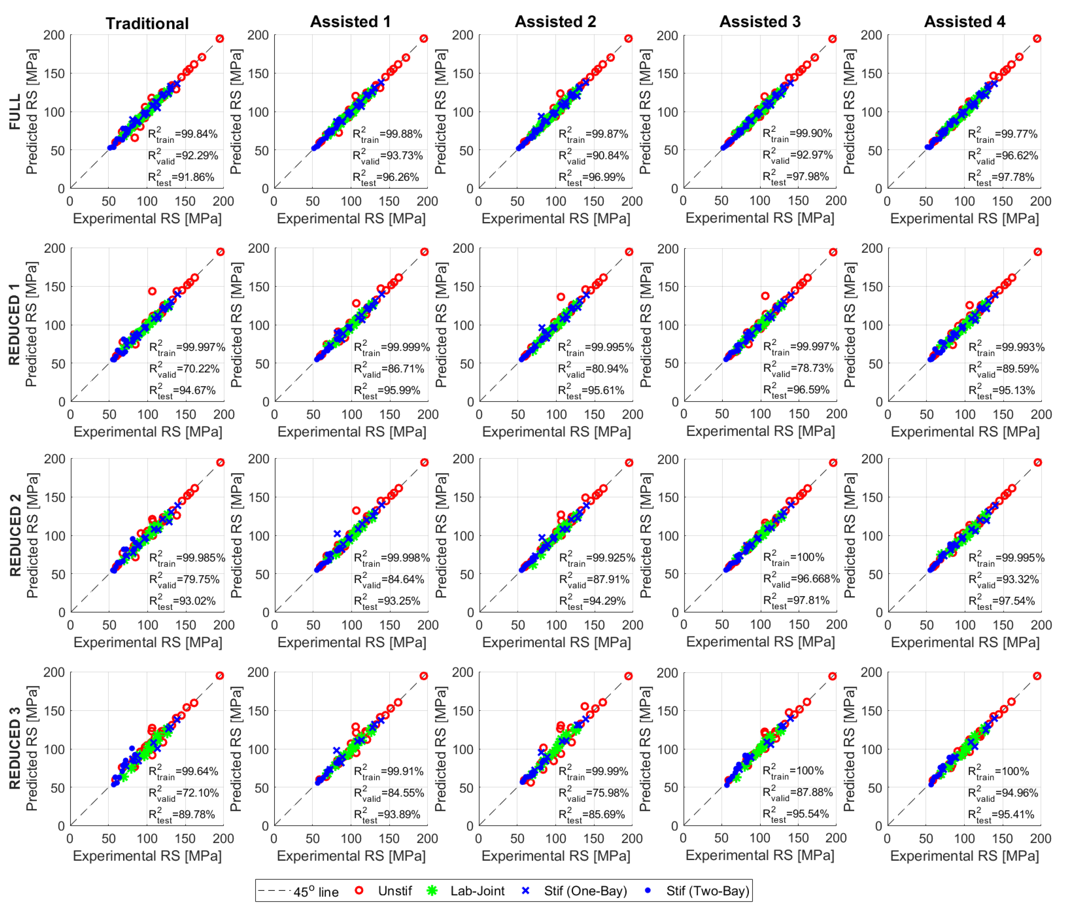
5. Results and Discussion

In this study, a novel assisted-ANN modeling is proposed and it is used for estimating the residual strength of aluminum panels with MSD cracks. The essence of the assisted approach being used here is to include some assistance parameters as ANN inputs, in addition to the traditional direct independent parameters (such as geometric quantities, material properties, configuration, etc.) typically used as inputs to the ANN model. These assistance parameters come from the known analytical input/output relations and are intended to help the ANN to better capture the complex input/output relations when the size of the training dataset is relatively small.

It is important to stress here that data preparation is crucial before the data can be utilized it in ANN modeling [7]. Several steps associated with data preparation are conducted on the current experimental data. Firstly, proper data selection and classification. This step is manifested in: (i) the careful selection of the model inputs for both the traditional approach and the proposed assisted approach, (ii) the adoption of cross-validation procedure where 80 random combinations are used for the training, validation and testing datasets, and (iii) the adoption of partially randomized selection where some selected data points in the training dataset are fixed to cover the upper and lower limits of each of the input parameters. Secondly, data preprocessing. Herein, only complete data are selected from literature, outliers are checked and excluded whenever found, and the output parameter values for some data points are formatted in terms of the stress rather than the load values. Thirdly, data transformation. Because of having one output parameter, normalizing or scaling was not necessary. However, it is worth mentioning here that in order to make the comparison of the relative weight of the inputs across the different scenarios easier; the relative weights are normalized for all scenarios in the different training datasets (as seen in Section 5.3).

5.1. Assisted-ANN Performance for Different Learning Algorithms

The ANN optimization procedure, described previously in Section 4.4, is carried out for the five modeling scenarios (traditional and the four assistance levels) used in this investigation. For each scenario, 80 ANNs are developed using the 80 random training datasets, and the optimum ANN configuration is identified based on the MAE_P value (averaged value for the 80 different random combinations) for the validation datasets. When using the testing datasets for evaluating the performance of the ANN, in addition to the MAE_P, two additional performance metrics (RMSE_P and R²) are also taken into consideration for determining the goodness of the residual strength predictions. For the traditional and all four assistance levels, the BR learning algorithm, along with the Elliot symmetric sigmoid (elliotsig) activation function, gives the best prediction performance. As for the optimum number of nodes in the hidden layer, it varies from case to case. The LM and SGC learning algorithms are ranked second and third, respectively, in terms of prediction accuracy. Thought, the BR learning algorithm results in the best prediction performance and will be adopted henceforth; however, it is also important to observe the effect of the assisted approach when used along with the different learning algorithms.

Table 2. Performance metrics for each learning algorithm using the traditional and assisted ANN modeling approaches (averages for the 80 random combinations of the testing dataset).

Scenario	BR			LM			SGC
	MAEP [%]	RSMEP [%]	R2 [%]	MAEP [%]	RSMEP [%]	R2 [%]	MAEP [%]	RSMEP [%]	R2 [%]
Traditional	3.8	5.51	92.39	5.59	7.89	81.19	7.65	10.33	75.94
Assisted 1	3.76	5.42	92.61	5.56	7.92	84.56	6.41	8.67	83.32
Assisted 2	3.45	5.04	93.16	4.86	6.8	87.89	6.05	8.16	84.49
Assisted 3	3.13	4.26	95.14	4.42	6.17	89.85	5.52	7.22	87.96
Assisted 4	2.97	4.07	96.21	3.31	4.2	96.04	4.13	5.48	92.9

lists the values of the three performance metrics obtained using the BR, LM and SGC algorithms for the traditional and the four assisted scenarios. In each case, the shown values are for the optimum configuration (best activation function and number of hidden nodes), and each value is the average for the 80 random combinations of the testing dataset. As can be seen from the table, improvement can be clearly observed in the MAE_P, RMSE_P and R² values for the four assisted scenarios as compared to the traditional scenario. Also, this improvement can be observed for the three learning algorithms. The improved results associated with the assisted scenarios indicate that, though dependency may exist between the direct independent input parameters and assistance parameters; the developed ANN model did not trap into local optima nor did it hide important input-output relationships. Also, the results show that the addition of the assistance parameters did not add significant noise into the model. Furthermore, the highly accurate results obtained using the testing dataset, also indicate that the ANN model did not experience overfitting during the learning process; on the contrary, it has learned to generalize to new situations.

To further illustrate the accuracy improvement resulting from using the assisted approach, Figure 3 is developed using the MAE_P values given in Table 2. From the figure, it can be seen that for any of the five scenarios, the BR gives the best accuracy followed by the LM then the SGC. The figure also shows that, for all three learning algorithms, the accuracy gradually improves as the assistance level increases (from assisted 1 to assisted 4). This gradual accuracy improvement is consistent with the logic of assigning the assistance parameters being used at the different assistance levels, where at each level, a higher-order assistance parameter is used (as previously explained in Section 4.2). In order to quantify the accuracy improvement obtained using the four assistance levels, the error (MAE_P) reduction relative to the traditional approach is calculated and shown in the bottom part of Figure 3.

By inspecting the relative error reduction values, it can be clearly observed that, in general, the heights values of error reduction are associated with the SGC algorithm, followed by the LM and BR algorithms, respectively. For instance, at assistance level 4, the relative error reduction for the SGC, LM and BR are −46.1%, −40.9% and −21.8%, respectively. This observation is rather interesting where it indicates that the accuracy improvement attained using the assisted approach becomes more pronounced when the original error of the traditional approach is higher. It is probably worth to mention here that the computer CPU time required to train and optimize the ANN using these three learning algorithms differs significantly. In terms of the run time, the SGC algorithm is the fastest while the BR is the slowest. For comparison purposes and to get a sense of the computational burden difference, taking the SCG as a reference, the relative run times for LM and BR are 2× and 104×, respectively.

The results presented in Table 2 and Figure 3 are averaged values for the 80 random combinations of the testing datasets. However, the calculated performance metrics are somewhat different for each of the 80 testing datasets combinations. To get a closer look at the results obtained using the individual datasets, Figure 4 shows exemplary results for one of the 80 testing datasets combinations (it contains 19 data points, and the sample ID for each data point is indicated in the figure). The upper part of Figure 4 shows the experimental residual strength value for each sample alongside with the ANN predictions obtained using the traditional approach and assisted 3 and 4 scenarios (assisted 1 and 2 are not shown in order not to congest the figure). The lower part of the figure shows the magnitude of error in the predicted residual strength using the traditional and the two assisted scenarios. The figure shows that the ANN residual strength predictions obtained using the two assisted scenarios are superior to the predictions obtained using the traditional approach for almost all the shown samples.

5.2. Effect of Smaller Training Dataset Size

The results presented in the previous section are obtained using full-size training datasets (each containing 75 data points). Thought this dataset size is relatively small, it is important to find out the effect of the assisted approach as the size of the training datasets gets even smaller. Thus, three progressively reduced training dataset sizes are also investigated. The three reduced training dataset sizes are: reduced-1 (48 data points), reduced-2 (35 data points) and reduced-3 (22 data points). For the reduced size datasets investigation, only the BR learning algorithm is used since it gives the best performance.

Table 3. Performance metrics for the reduced size training datasets using the traditional and assisted ANN modeling approaches (averages for the 80 random combinations of the testing dataset).

Scenario	Reduced 1 (48)			Reduced 2 (35)			Reduced 3 (22)
	MAEP [%]	RSMEP [%]	R2 [%]	MAEP [%]	RSMEP [%]	R2 [%]	MAEP [%]	RSMEP [%]	R2 [%]
Traditional	4.68	6.52	88.73	5.55	7.52	85.77	6.86	9.54	80.97
Assisted 1	4.67	6.61	89.59	5.1	7.01	87.65	4.51	5.93	90.24
Assisted 2	4.16	5.82	91.46	4.65	6.32	90.2	4.52	5.92	90.97
Assisted 3	3.55	4.88	93.91	3.84	5.33	92.85	4.63	6.21	91.64
Assisted 4	3.46	4.54	95.21	3.46	4.52	95.16	4.26	5.83	92.81

lists the values of the three performance metrics obtained using the reduced training dataset sizes for the traditional and the four assisted scenarios. From the table, it can be seen that for the three reduced training dataset sizes, the MAE_P, RMSE_P and R² values for the four assisted scenarios are clearly superior to those of the traditional approach. Closer inspection of the results listed in the table shows that for reduced-1 and reduced-2 dataset sizes, the accuracy gradually improves as the assistance level gets higher; whereas, for reduced-3 dataset size, the results associated with assisted 1, 2 and 3 scenarios are fairly close to each other. The general trend for accuracy improvement for the different training dataset sizes can be better observed by referring to Figure 5. Similar to Figure 3, the upper part of Figure 5 shows MAE_P values obtained using the traditional and assisted scenarios associated with the different dataset sizes, while the lower part of the figure shows the error reduction of the assisted scenarios relative to the traditional approach. The data presented in the figure for the full-size dataset are obtained from Table 2. As expected, the figure shows that, in general, as the size of the training dataset gets smaller, the ANN predictions become less accurate. From the figure, it can be seen that for all dataset sizes, except reduced-3, the accuracy of the ANN predictions gradually improves as the assistance level increases. It can also be seen that the relative error reduction increases as the dataset size gets smaller. This observation clearly indicates that the proposed assisted-ANN approach is more effective in improving the accuracy for smaller size training datasets. For the reduced-3 training dataset size, the figure shows that the situation is slightly different than the larger dataset sizes. In this case, all the four assisted scenarios give clearly better accuracy than the traditional approach; however, the relative error reduction resulting from assisted scenarios 1, 2 and 3 is relatively high, and the error reduction values for the three scenarios are fairly close to each other. It is probably worth mentioning here that for the reduced-3 training dataset size, all the data points are manually selected; while for the larger dataset sizes (reduced-1 and reduced-2), some of the data points are chosen randomly. As mentioned previously, the manually selected data points are all at either the upper or lower limit values of the different inputs (lead crack length, ligament length, etc.), and do not include intermediate values. Most likely, this difference in the nature of the data points for reduced-3 is what cussed the difference in relative error reduction trend. The fact that the relative error reduction achieved using the four assisted scenarios is fairly high (>30%) for reduced-3 training dataset size, indicates that the assisted approach helped the ANN to properly capture the input/output relations, though no intermediate values (for some of the inputs) are available in the training dataset. This observation further confirms the importance of using the proposed assisted approach for small size datasets.

In order to further examine the effect of the assisted approach for smaller dataset sizes, Figure 6 shows exemplary results for one of the 80 testing datasets combinations (the same testing dataset shown previously in Figure 4). The upper part of the figure shows the experimental residual strength value and the ANN predictions (for traditional, assisted 3 and 4 scenarios); while the lower part shows the magnitude of error in ANN predictions. The figure shows that for most of the samples shown in the figure (15 out of 19) the ANN residual strength predictions obtained using the two assisted scenarios are superior to the predictions obtained using the traditional approach. It should be clear here that the purpose of Figure 6 is to observe the overall predictions accuracy for the individual samples. The fact that the traditional approach predictions for some of the samples (U-25 for instance) are more accurate, does not affect the overall conclusions which are based on the averages for large numbers of data points.

Finally, in order to visualize the overall accuracy improvement for the ANN residual strength predictions when using the assisted approach, the correlation between the experimental results and ANN predictions for the different training dataset sizes are shown in Figure 7. The data shown in this figure are for one of the 80 datasets combinations, and the figure shows the correlation for all data points (training, validation and testing). In all of the subfigures, the points are distributed uniformly above and below the 45-degrees line; this indicates that there is no over-or-under prediction tendency in the ANN predictions, and the prediction errors are fairly random (no systematic error is observed). In this type of figures, the closer the points to the 45-degrees line, the more accurate the predictions are. For all the different training dataset sizes, it can be seen that as we transition from one subfigure to the next (left to right direction) the data points become closer to the 45-degree line. This observation is another indication of the accuracy improvement attained using the assisted approach scenarios. It can also be observed from the figure that, as we transition from one subfigure to the one below, the data points tend to get farther from the 45-degree line. This observation gives further verification that the accuracy decreases as the training dataset size becomes smaller. It can also be seen from the figure that there is no noticeable difference in accuracy for the different panel configurations (unstiffened, stiffened, etc.) since all the data are clustered close to the 45-degrees line. The coefficient of determination (R²) values for the training, validation, and testing datasets are also shown in each of the subfigures. It can be noticed that the coefficient of determination for the training datasets are clearly higher than those for the validation and training datasets. In fact, this trend is quite normal since the training data are already “seen” by the ANN (since they are used for training); therefore, the ANN can predict the residual strength for the training datasets more accurately that the “unseen” validation and testing datasets.

5.3. ANN Inputs Relative Importance

To better understand how the proposed assisted-ANN modeling approach improves the prediction accuracy and enables the network to be trained efficiently using small datasets, it is essential to look at the effect of the added assistance inputs on the internal parameters (i.e., the weights) of the ANN. Specifically, the contribution of each input in the ANN’s residual strength predictions can be quantified by resorting to the connection weights (CW) algorithm [64]. The relative weight of any of the ANN inputs basically reflects its relative importance, and therefore the different inputs can be ranked based on the relative weight values [65]. That is, the evolution of the ANN internal parameters considering the different scenarios investigated in this work is embedded in the quantification of the relative weight values. The CW algorithm [64] uses the ultimate inputs-hidden connection weights ($W_{xy}$), from $x$-th input node ($x=1,\dots ,X$) to $y$-th hidden node ($y=1,\dots ,H$), and the ultimate hidden-output connection weights ($W_{yz}$), from $y$-th hidden node ($y=1,\dots ,H$) to the $z$-th output node ($z=1$), obtained for the optimum ANN models of the different scenarios to assess the Relative Weight (${\mathrm{RW}}_x$) of each $x$-th ANN input ($x=1,\dots ,X$) as follows:

$${\mathrm{RW}}_x=\left|{\displaystyle \sum }_{y=1}^H{W}_{xy}{W}_{yz}\right|$$

(10)

where ${\mathrm{RW}}_x$ is the “absolute” relative weight of the $x$-th input node and ${\displaystyle \sum }_{y=1}^H{W}_{xy}{W}_{yz}$ is the sum of the product of the ultimate weights of the connections from the $x$-th input node to hidden nodes ($W_{xy}$) with the connections from the hidden nodes to the output node ($W_{yz}$). It is worth mentioning that the sum of products used here is the average sum of products calculated over the 80 cross-validation combinations of each ANN scenario. The absolute value is taken here because the sign of the relative weight is not considered when ranking the inputs according to their importance. The relative weights are calculated for each of the ANN inputs used in the traditional approach and the four assisted approach scenarios. In order to make the comparison of the relative weight of the inputs across the different scenarios easier, the relative weights are normalized for each scenario. After normalization, the total normalized relative weights for all inputs for any of the different scenarios is equal to 1. The normalized relative weights calculations are also done for the different training dataset sizes, and all the data are graphically represented in Figure 8. The first seven inputs (“a” to “config ID”) are the direct independent inputs, and they are common for the traditional and the four assisted approach scenarios. The last four inputs are the assistance parameters where one or more of them is used at each of the four assistance levels (see Table 1). By inspecting the different parts of the figure, corresponding to the different training dataset sizes, it can be seen that the overall trends seen in these parts are fairly similar (except for few minor differences in the relative weights of some inputs). The figure shows that for the assisted approach scenarios, starting from assistance level 1 up to 4, the relative weights of the assistance input parameters are always increasing (note that for assistance level 3, two assistance parameters are used and thus, their weights are added together). As a matter of fact, this observation is consistent with the logic behind assigning the assistance parameters for the different assistance levels according to the theoretical definitions of these parameters (as explained in Section 4.2). The increase in the relative weight of the assistance parameters comes at the expense of the relative weights of the direct independent inputs (since the total weight for all inputs is 1). For instance, at assistance level 4, the relative weight of the assistance input parameter (σ_LU) is about 0.7, which leaves only about 0.3 relative weight for all the seven independent inputs. It can also be seen from the figure that although the relative weights of all the direct inputs is reduced as the assistance parameters are added, some of the inputs are clearly affected more than the others. If we, for instance, consider the “config ID”, which is used to identify the four different test panel configurations being used in this study, it can be seen that the relative weight of this input immediately drops and becomes close to zero for all the assisted approach scenarios. This drop is rather expected since all of the assistance parameters being used here account for the panel configuration more explicitly. When the weight of any of the inputs becomes very close to zero, this means that this parameter can be excluded from the ANN inputs. However, as previously mentioned in Section 4.2, the essence of the assisted approach being proposed here is to add the necessary assistance parameters to the ANN inputs without deleting any of the direct independent inputs. As such, the ANN itself will recognize the importance of each of the inputs and give it its appropriate weight. Indeed, the results presented here show that the ANN is able to do that successfully. Also, the results presented here clearly show that the ANN is able to handle the different inputs without compromising the performance, though some of the inputs (i.e., the assistance parameters) are dependent on other inputs.

Table 4. Ranking of the different ANN inputs based on their importance (relative weight) for the full size training datasets (results are based on averages for the 80 random combinations of the training dataset).

Scenario	Direct Independent Inputs							Assistance Input Parameters
	a	l	L	W	Astf	σy	Config ID	βP-config	βa	βℓ	σLU
Traditional	2	4	1	7	6	5	3	-	-	-	-
Assisted 1	1	4	2	6	8	5	7	3	-	-	-
Assisted 2	1	6	2	7	8	4	5	-	3	-	-
Assisted 3	3	5	4	9	7	6	8	-	1	2	-
Assisted 4	8	4	2	5	6	7	3	-	-	-	1

gives the ranking of the different ANN inputs for the traditional and assisted approach scenarios (for the full-size training dataset) based on their relative weights shown in Figure 8. The table shows that the assistance parameters ranking is clearly higher than most of the other direct inputs. For assistance levels 1 and 2, the assistance parameters are ranked third, and they go to the first rank for assistance levels 3 and 4. Other than the assistance parameters, the two most important inputs are the ligament length (L) and the lead crack half-length (a). However, it should be noticed that at assistance level 4, the importance of “a” diminishes (it goes to rank 8) and “L” remains as the only significant input (of course after σ_LU). In fact, at this assistance level, the ANN benefits from the Linkup model’s ability to capture the general trend of the residual strength, and the ANN basically corrects the Linkup model predictions based on the experimental results. The fact that the most significant input for this assisted scenario is “L”, means that the ligament length is the main parameter that causes error in the Linkup model predictions (because of inaccurate estimation of the plastic zone size). This observation is actually in agreement with the findings of Smith et al. [30,44,45] where the empirical corrections they developed for the Linkup model are a function of the ligament length alone.

Finally, it is probably worth mentioning here that when using the traditional approach, accurate predictions can be made only for panels of the exact same configurations used in training. On the contrary, adopting the proposed assisted approach can help in extending the applicability of the ANN model to panel configurations different from those used in training. If we consider for instance the one-bay stiffened panels for which 21 data points are available (panel IDs S-1 to S-21), and all of them have the same spacing between the stiffeners (305 mm). In fact, several parameters related to the stiffeners (such as the stiffeners’ cross-sectional area and spacing, fasteners’ stiffness and spacing, etc.) will affect the residual strength. If all of these parameters are to be included as inputs for the ANN, at least tens of training datasets (if not hundreds) will be required for the network to capture the effects of all these input parameters on the output. In contrast, in the assisted approach, a single input parameter (β_s), which combines the effect of all of these individual parameters on the SIF, can be included as an assistance input parameter. As such, the ANN will be able to better recognize the effect of the stiffeners and make accurate predictions without the need for a huge training dataset. In addition, the network will also be able to predict the residual strength for stiffened panels even if the spacing between the stiffeners is different from what is used in the training dataset since the assistance parameter β_s completely accounts for the geometry of the stiffeners. The same idea is also true for the other higher-level SIF geometric correction factors being used here as assistance parameters. For instance, the lead-crack overall correction factor (β_a), which is used at assistance level 2, combines different effects together. For a stiffened panel, β_a combines the stiffeners effect, the panel width effect, and the interaction effect of the MSD cracks on the lead crack. Accordingly, the inclusion of this assistance parameter among the inputs makes it easier for the ANN to recognize the complex interactions between the different geometric input parameters. Therefore, it further improves the residual strength predictions’ accuracy.

6. Concluding Remarks

It is widely believed that one of the advantages of ANNs is their ability to model complex non-linear relationships between several input/output parameters, without any need for prior knowledge of the nature of the relationships between these parameters. While this is generally true, however a large training dataset (usually hundreds of data points) will be required for the ANN to fully capture such complex non-linear relationships. In many engineering applications, such as fracture mechanics for instance, the input/output relations are complex and highly non-linear; and at the same time, the curation of large experimental datasets is usually not feasible. This paper introduces a novel assisted-ANN modeling approach that enables the ANN to be trained using small datasets and still achieve high prediction accuracy. This approach is demonstrated, and its capabilities are investigated by applying it for evaluating the residual strength of panels with MSD cracks. The purpose of the assisted-ANN modeling approach proposed here is to assist the ANN learning process, when the training dataset is relatively small, and therefore improve the accuracy of the output predictions. This is done by including additional inputs (called assistance parameters) that are obtained from the known analytical input/output relations. So, in essence, our approach merges the well-known and well-established analytical relations (between the different input/output parameters) with the ANN technique to improve the ability of ANN to estimate the residual strength of panels with MSD cracks. The inputs that are usually used in ANN modeling are geometry and material related, and they are “independent” from each other. In contrary to the inputs used in the traditional approach, the added assistance parameters being used in the assisted approach are basically “dependent” on the other input parameters, and they are calculated using the existing analytical relations (or obtained using computational techniques). The results presented in this paper demonstrate that the assisted-ANN modeling approach clearly improves the residual strength predictions’ accuracy, in comparison to the traditional approach. Using the assisted approach, an average prediction error (MAE_P) of less than 3% is achieved. Also, the relative reduction in the prediction error, compared to the traditional approach, reached up to 46% in some cases. The main conclusions of this study can be summarized in the following points:

• Different types of parameters can be used as assistance parameters, and one or more assistance parameters can be used at the same time. The assistance parameters can be obtained using any well-established relation that partially or fully relate some (or all) of the inputs with the output (e.g., the SIF correction factors are partial relations while the linkup model is a full relation). The amount of the achieved accuracy improvement depends on the level and the accuracy of the assistance parameter(s) being used.
• The fact that the SIF correction factors can be successfully used as assistance input parameters makes the proposed assisted-ANN approach to be useful in a very wide variety of fracture mechanics applications (both for fatigue crack growth and static fracture). The assisted-ANN approach should prove to be very helpful in cases where the number of data points available for training the ANN is limited, which is generally the case in many experimental investigations in the fracture mechanics field.
• The lower the accuracy of the predictions obtained using the traditional approach, the more the improvement that is achieved using the assisted approach. For the SGC algorithm (it gives the least accurate results), the relative error reduction achieved by the assisted approach reached −46%; whereas for the BR algorithm (it gives the most accurate results), the relative error reduction achieved by the assisted approach reached −22% only.
• As the size of the training dataset gets smaller, the assistance input parameters will play a more significant role in improving the ANN performance. The results show that the relative error reduction generally increases as the size of the training dataset gets smaller. For the 22 data points training dataset, the achieved relative error reduction by the assisted approach reached −37%; whereas for the 75 data points training dataset, the achieved relative error reduction by the assisted approach reached −22% only.
• In the proposed assisted approach, all the direct independent inputs used in the traditional approach are still used and the assistance parameter(s) is/are used as additional input(s). The added assistance parameter(s) will influence the internal configuration of the ANN, especially the neurons’ connection weights. When an assistance parameter is added to the inputs, its relative weight becomes clearly higher than most (or all) of the other direct independent inputs. This shows the importance of adding the assistance parameter and the significant role it plays in the internal ANN structure. Also, when an assistance parameter is added, the relative weight of some of the inputs is reduced significantly, which means that the assistance parameter is taking over their role. Usually, the inputs with very small relative weights are deleted; however, our results show that to be not necessary since the ANN can recognize the importance of each of the inputs and give it its appropriate weight. Furthermore, the results show that the ANN is able to efficiently handle all the different types of inputs whether they are independent or dependent.

References

1. Haykin, S. Neural Networks: A Comprehensive Foundation; Prentice-Hall Inc.: Upper Saddle River, NJ, USA, 2007. [Google Scholar]
2. He, W.; Yan, Z.; Sun, Y.; Ou, Y.; Sun, C. Neural-Learning-Based Control for a Constrained Robotic Manipulator with Flexible Joints. IEEE Trans. Neural Netw. Learn. Syst. 2018, 29, 5993–6003. [Google Scholar] [CrossRef] [PubMed]
3. Elsheikh, A.H.; Sharshir, S.W.; Elaziz, M.A.; Kabeel, A.; Guilan, W.; Zhang, H. Modeling of solar energy systems using artificial neural network: A comprehensive review. Sol. Energy 2019, 180, 622–639. [Google Scholar] [CrossRef]
4. Al-Dahidi, S.; Ayadi, O.; Alrbai, M.; Adeeb, J. Ensemble Approach of Optimized Artificial Neural Networks for Solar Photovoltaic Power Prediction. IEEE Access 2019, 7, 81741–81758. [Google Scholar] [CrossRef]
5. Cao, J.; Fang, Z.; Qu, G.; Sun, H.; Zhang, D. An accurate traffic classification model based on support vector machines. Int. J. Netw. Manag. 2017, 27, e1962. [Google Scholar] [CrossRef]
6. Mehdy, M.M.; Ng, P.Y.; Shair, E.F.; Saleh, N.I.M.; Gomes, C. Artificial Neural Networks in Image Processing for Early Detection of Breast Cancer. Comput. Math. Methods Med. 2017, 2017, 1–15. [Google Scholar] [CrossRef] [Green Version]
7. Mendes, N.; Ferrer, J.; Vitorino, J.; Safeea, M.; Neto, P. Human Behavior and Hand Gesture Classification for Smart Human-robot Interaction. Procedia Manuf. 2017, 11, 91–98. [Google Scholar] [CrossRef]
8. Yamanaka, A.; Kamijyo, R.; Koenuma, K.; Watanabe, I.; Kuwabara, T. Deep neural network approach to estimate biaxial stress-strain curves of sheet metals. Mater. Des. 2020, 195, 108970. [Google Scholar] [CrossRef]
9. Altarazi, S.; Ammouri, M.; Hijazi, A.L. Artificial neural network modeling to evaluate polyvinylchloride composites’ properties. Comput. Mater. Sci. 2018, 153, 1–9. [Google Scholar] [CrossRef]
10. Altarazi, S.; Allaf, R.M.; Al-Hindawi, F. Machine Learning Models for Predicting and Classifying the Tensile Strength of Polymeric Films Fabricated via Different Production Processes. Materials 2019, 12, 1475. [Google Scholar] [CrossRef] [Green Version]
11. Dagli, C.H. Artificial Neural Networks for Intelligent Manufacturing; Springer Science & Business Media: Dordrecht, The Netherlands, 2012. [Google Scholar]
12. Ashhab, M.S.; Breitsprecher, T.; Wartzack, S. Neural network based modeling and optimization of deep drawing—Extrusion combined process. J. Intell. Manuf. 2014, 25, 77–84. [Google Scholar] [CrossRef]
13. Nasiri, S.; Khosravani, M.R.; Weinberg, K. Fracture mechanics and mechanical fault detection by artificial intelligence methods: A review. Eng. Fail. Anal. 2017, 81, 270–293. [Google Scholar] [CrossRef]
14. Feng, S.; Zhou, H.; Dong, H.B. Using deep neural network with small dataset to predict material defects. Mater. Des. 2019, 162, 300–310. [Google Scholar] [CrossRef]
15. Balcioglu, H.E.; Seçkin, A.Ç.; Aktas, M. Failure load prediction of adhesively bonded pultruded composites using artificial neural network. J. Compos. Mater. 2016, 50, 3267–3281. [Google Scholar] [CrossRef]
16. Hakim, S.J.S.; Razak, H.A. Structural damage detection of steel bridge girder using artificial neural networks and finite element models. Steel Compos. Struct. 2013, 14, 367–377. [Google Scholar] [CrossRef] [Green Version]
17. Janssens, O.; Slavkovikj, V.; Vervisch, B.; Stockman, K.; Loccufier, M.; Verstockt, S.; Van De Walle, R.; Van Hoecke, S. Convolutional Neural Network Based Fault Detection for Rotating Machinery. J. Sound Vib. 2016, 377, 331–345. [Google Scholar] [CrossRef]
18. Shu, J.; Zhang, Z.; González, I.; Karoumi, R. The application of a damage detection method using Artificial Neural Network and train-induced vibrations on a simplified railway bridge model. Eng. Struct. 2013, 52, 408–421. [Google Scholar] [CrossRef] [Green Version]
19. Nechval, K.N.; Nechval, N.A.; Bausova, I.; Skiltere, D.; Strelchonok, V.F. Prediction of fatigue crack growth process via artificial neural network technique. Int. J. Comput. 2006, 5, 21–32. [Google Scholar]
20. Hamdia, K.M.; Lahmer, T.; Nguyen-Thoi, T.; Rabczuk, T. Predicting the fracture toughness of PNCs: A stochastic approach based on ANN and ANFIS. Comput. Mater. Sci. 2015, 102, 304–313. [Google Scholar] [CrossRef]
21. Mortazavi, S.; Ince, A. An artificial neural network modeling approach for short and long fatigue crack propagation. Comput. Mater. Sci. 2020, 185, 109962. [Google Scholar] [CrossRef]
22. Seibi, A.; Al-Alawi, S. Prediction of fracture toughness using artificial neural networks (ANNs). Eng. Fract. Mech. 1997, 56, 311–319. [Google Scholar] [CrossRef]
23. Ince, R. Prediction of fracture parameters of concrete by Artificial Neural Networks. Eng. Fract. Mech. 2004, 71, 2143–2159. [Google Scholar] [CrossRef]
24. Spear, A.D.; Priest, A.R.; Veilleux, M.G.; Ingraffea, A.R.; Hochhalter, J.D. Surrogate Modeling of High-Fidelity Fracture Simulations for Real-Time Residual Strength Predictions. AIAA J. 2011, 49, 2770–2782. [Google Scholar] [CrossRef] [Green Version]
25. Pidaparti, R.M.; Jayanti, S.; Palakal, M.J. Residual Strength and Corrosion Rate Predictions of Aging Aircraft Panels: Neural Network Study. J. Aircr. 2002, 39, 175–180. [Google Scholar] [CrossRef]
26. Pidaparti, R. Aircraft structural integrity assessment through computational intelligence techniques. Struct. Durab. Health Monit. 2006, 2, 131. [Google Scholar]
27. Hijazi, A.; Al-Dahidi, S.; Altarazi, S. Residual Strength Prediction of Aluminum Panels with Multiple Site Damage Using Artificial Neural Networks. Materials 2020, 13, 5216. [Google Scholar] [CrossRef]
28. Swift, T. Widespread Fatigue Damage Monitoring: Issues and Concerns. In Proceedings of the 5th International Conference on Structural Airworthiness of New and Ageing Aircraft, Hamburg, Germany, 16–18 June 1993; pp. 113–150. [Google Scholar]
29. Hijazi, A.L. Residual Strength of Thin-Sheet Aluminum Panels with Multiple Site Damage. Ph.D. Thesis, Wichita State University, Wichita, KS, USA, 2002. [Google Scholar]
30. Smith, B.L.; Saville, P.A.; Mouak, A.; Myose, R.Y. Strength of 2024-T3 Aluminum Panels with Multiple Site Damage. J. Aircr. 2000, 37, 325–331. [Google Scholar] [CrossRef]
31. Smith, B.L.; Hijazi, A.L.; Haque, A.K.M.; Myose, R.Y. Strength of Stiffened 2024-T3 Aluminum Panels with Multiple Site Damage. J. Aircr. 2001, 38, 764–768. [Google Scholar] [CrossRef]
32. Hijazi, A.L.; Smith, B.L.; Lacy, T.E. Linkup Strength of 2024-T3 Bolted Lap Joint Panels with Multiple Site Damage. J. Aircr. 2004, 41, 359–364. [Google Scholar] [CrossRef]
33. Hijazi, A.L.; Lacy, T.E.; Smith, B.L. Comparison of Residual Strength Estimates for Bolted Lap-Joint Panels. J. Aircr. 2004, 41, 657–664. [Google Scholar] [CrossRef]
34. Xu, W.; Wang, H.; Wu, X.; Zhang, X.; Bai, G.; Huang, X. A novel method for residual strength prediction for sheets with multiple site damage: Methodology and experimental validation. Int. J. Solids Struct. 2014, 51, 551–565. [Google Scholar] [CrossRef] [Green Version]
35. Wu, S.; Zhou, X.-G.; Cao, G.-M.; Liu, Z.; Wang, G.-D. The improvement on constitutive modeling of Nb-Ti micro alloyed steel by using intelligent algorithms. Mater. Des. 2017, 116, 676–685. [Google Scholar] [CrossRef]
36. Qiao, L.; Liu, Y.; Zhu, J. Application of generalized regression neural network optimized by fruit fly optimization algorithm for fracture toughness in a pearlitic steel. Eng. Fract. Mech. 2020, 235, 107105. [Google Scholar] [CrossRef]
37. Candelieri, A.; Sormani, R.; Arosio, G.; Giordani, I.; Archetti, F. Assessing structural health of helicopter fuselage panels through artificial neural networks hierarchies. Int. J. Reliab. Saf. 2013, 7, 216. [Google Scholar] [CrossRef]
38. Li, D.-C.; Chen, L.-S.; Lin, Y.-S. Using Functional Virtual Population as assistance to learn scheduling knowledge in dynamic manufacturing environments. Int. J. Prod. Res. 2003, 41, 4011–4024. [Google Scholar] [CrossRef]
39. Shaikhina, T.; Khovanova, N.A. Handling limited datasets with neural networks in medical applications: A small-data approach. Artif. Intell. Med. 2017, 75, 51–63. [Google Scholar] [CrossRef]
40. Mao, R.; Zhu, H.; Zhang, L.; Chen, A.; Zhu, R.M.H. A New Method to Assist Small Data Set Neural Network Learning. In Proceedings of the Sixth International Conference on Intelligent Systems Design and Applications, Jinan, China, 16–18 October 2006; Volume 1, pp. 17–22. [Google Scholar]
41. Thomson, D.; Hoadley, D.; McHatton, J. Load Tests of Flat and Curved Panels with Multiple Cracks; Foster-Miller Draft Final Report; FAA Technical Center: Egg Harbor Township, NJ, USA, 1993. [Google Scholar]
42. Dewit, R.; Fields, R.J.; Mordfin, L.; Low, S.R.; Harne, D. Fracture Behavior of Large-Scale Thin-Sheet Aluminum Alloy; NIST Technical Report 5661; NIST: Gaithersburg, MD, USA, 1995.
43. Anderson, T.L. Fracture Mechanics: Fundamentals and Applications; CRC Press: Boca Raton, FL, USA, 2017. [Google Scholar]
44. Smith, B.L.; Hijazi, A.L.; Myose, R.Y. Strength of 7075-T6 and 2024-T3 Aluminum Panels with Multiple-Site Damage. J. Aircr. 2002, 39, 354–358. [Google Scholar] [CrossRef]
45. Smith, B.L.; Flores, T.L.Z.; Hijazi, A.L. Link-Up Strength of 2524-T3 and 2024-T3 Aluminum Panels with Multiple Site Damage. J. Aircr. 2005, 42, 535–541. [Google Scholar] [CrossRef]
46. Dandy, G.; Maier, H.R. Review of Input Variable Selection Methods for Artificial Neural Networks. Artif. Neural Netw. Methodol. Adv. Biomed. Appl. 2011, 10, 16004. [Google Scholar] [CrossRef] [Green Version]
47. Bowden, G.J.; Dandy, G.C.; Maier, H.R. Input determination for neural network models in water resources applications. Part 1—Background and methodology. J. Hydrol. 2005, 301, 75–92. [Google Scholar] [CrossRef]
48. May, R.; Dandy, G.C.; Maier, H.R.; Nixon, J.B. Application of partial mutual information variable selection to ANN forecasting of water quality in water distribution systems. Environ. Model. Softw. 2008, 23, 1289–1299. [Google Scholar] [CrossRef]
49. Li, K.; Hu, C.; Liu, G.; Xue, W. Building’s electricity consumption prediction using optimized artificial neural networks and principal component analysis. Energy Build. 2015, 108, 106–113. [Google Scholar]
50. Yang, C.; Kim, Y.; Ryu, S.; Gu, G.X. Prediction of composite microstructure stress-strain curves using convolutional neural networks. Mater. Des. 2020, 189, 108509. [Google Scholar] [CrossRef]
51. Yu, S.; Chou, K. Integration of independent component analysis and neural networks for ECG beat classification. Expert Syst. Appl. 2008, 34, 2841–2846. [Google Scholar] [CrossRef]
52. Yadav, A.K.; Malik, H.; Chandel, S. Selection of most relevant input parameters using WEKA for artificial neural network based solar radiation prediction models. Renew. Sustain. Energy Rev. 2014, 31, 509–519. [Google Scholar] [CrossRef]
53. Dolara, A.; Grimaccia, F.; Leva, S.; Mussetta, M.; Ogliari, E. A Physical Hybrid Artificial Neural Network for Short Term Forecasting of PV Plant Power Output. Energies 2015, 8, 1138–1153. [Google Scholar] [CrossRef] [Green Version]
54. US Department of Defense. Handbook: Metallic Materials and Elements for Aerospace Vehicle Structures; Military Handbook No. MIL-HDBK-5H, Section 5; US Department of Defense: Arlington, VA, USA, 1998.
55. Bendat, J.S.; Piersol, A.G. Random Data: Analysis and Measurement Procedures; John Wiley & Sons: Hoboken, NJ, USA, 2011. [Google Scholar]
56. Poe, C., Jr. Stress Intensity Factor for a Cracked Sheet with Riveted and Uniformly Spaced Stringers; NASA/TR 1971, R-358; NASA: Washington, DC, USA, 1985.
57. Rooke, D.P.; Cartwright, D.J. Compendium of Stress Intensity Factors; Ministry of Defence: London, UK, 1976.
58. Swift, T. Fracture Analysis of Stiffened Structure. In Damage Tolerance of Metallic Structures: Analysis Methods and Applications; ASTM International: West Conshohocken, PA, USA, 1984. [Google Scholar]
59. Baghirli, O. Comparison of Lavenberg-Marquardt, Scaled Conjugate Gradient and Bayesian Regularization Backpropagation Algorithms for Multistep Ahead Wind Speed Forecasting Using Multilayer Perceptron Feedforward Neural Network. Master’s Thesis, Uppsala University, Uppsala, Sweden, 2015. [Google Scholar]
60. Peters, S.O.; Sinecen, M.; Gallagher, G.R.; Pebworth, L.A.; Hatfield, J.S.; Kizilkaya, K. 1690 Comparison of linear model and artificial neural network using antler beam diameter and beam length of white-tailed deer (Odocoileus virginianus). J. Anim. Sci. 2016, 94, 823–824. [Google Scholar] [CrossRef]
61. Al-Dahidi, S.; Ayadi, O.; Adeeb, J.; Louzazni, M. Assessment of Artificial Neural Networks Learning Algorithms and Training Datasets for Solar Photovoltaic Power Production Prediction. Front. Energy Res. 2019, 7, 130. [Google Scholar] [CrossRef] [Green Version]
62. Arora, M.; Ashraf, F.; Saxena, V.; Mahendru, G.; Kaushik, M.; Shubham, P. A Neural Network-Based Comparative Analysis of BR, LM, and SCG Algorithms for the Detection of Particulate Matter. In Advances in Interdisciplinary Engineering; Springer: Singapore, 2019; pp. 619–634. [Google Scholar]
63. Hagan, M.T.; Demuth, H.B.; Beale, M.H. Neural Network ToolboxTM 6 User’s Guide; MathWorks: Natick, MA, USA, 2015. [Google Scholar]
64. Olden, J.D.; Jackson, D.A. Illuminating the “black box”: A randomization approach for understanding variable contributions in artificial neural networks. Ecol. Model. 2002, 154, 135–150. [Google Scholar] [CrossRef]
65. Ibrahim, O.M. A comparison of methods for assessing the relative importance of input variables in artificial neural networks. J. Appl. Sci. Res. 2013, 9, 5692–5700. [Google Scholar]
Figure 1. Illustration of the MSD test panel geometry and the crack-tip plastic zone.
Applsci 10 08255 g001
Figure 2. The ANN structure: (a) traditional direct independent inputs approach, (b) assisted approach with calculated assistance parameters.
Applsci 10 08255 g002
Figure 3. The effect of the assisted approach on the ANN prediction accuracy using the different learning algorithms. The MAEP values for the traditional and assisted approaches residual strength predictions (top), together with the error reduction of the assisted approach relative to the traditional approach (bottom). Averaged results for the 80 random combinations of the testing dataset.
Applsci 10 08255 g003
Figure 4. The experimental residual strength values along with the predictions obtained by the ANN model for the traditional and assisted approaches (assisted 3 and 4 only) for one of the testing datasets using the BR algorithm (top), together with the residual strength prediction errors (bottom). The shown ANN predictions are for the best one of the 80 random combinations of the testing datasets.
Applsci 10 08255 g004
Figure 5. The effect of the assisted approach on the ANN prediction accuracy using the different learning algorithms. The MAEP values for the traditional and assisted approaches residual strength predictions (top), together with the error reduction of the assisted approach relative to the traditional approach (bottom). Averaged results for the 80 random combinations of the testing dataset.
Applsci 10 08255 g005
Figure 6. The experimental residual strength values along with the predictions obtained by the ANN model built using the reduced size training dataset (reduced 3) for the traditional and assisted approaches (assisted 3 and 4 only) for one of the testing datasets (top), together with the residual strength prediction errors (bottom). The shown ANN predictions are for the same testing dataset used in Figure 4.
Applsci 10 08255 g006
Figure 7. Effect of the assisted modeling approach and training dataset size on the correlation of ANN predictions with experimental residual strength values (for all data points used for training, validation, and testing). The effect of the assisted approach is observed when moving from left to right, while the effect of training dataset size reduction is observed when moving from top to bottom. The shown ANN predictions are for one of the 80 training/validation/testing datasets random combinations.
Applsci 10 08255 g007
Figure 8. Normalized relative weights of the different ANN inputs for the traditional and assisted approach at the different training dataset sizes (results are based on averages for the 80 random combinations of the training dataset).
Applsci 10 08255 g008