Modeling and Forecasting Gender-Based Violence through Machine Learning Techniques

 ,
,  ,
,  ,
, 

Abstract
1. Introduction
2. Related Works
3. Feature Selection and Forecasting Time Series
3.1. Feature Selection Techniques
- -
- Wrapper methods
- -
- Filter methods
- -
- Embedded methods
3.2. Forecasting
4. Database, Available Features, and Target to Be Forecasted
- -
- Territorial: We study the time-series data for the entire country but also some provinces as examples, in order to test the validation of our purpose.
- -
- Date and season: We will explore the evolution of GBV within years, month by month. We will also include the quarter to evaluate the influence of the season, as indicated by previous works [59].
- -
- Demography and population: Considering population can offer insights into the influence of big population areas, but some changes in demography can also provide explanations of the course of couples [60]. In this manner, marriages, separations, and births are included, but also the proportion of men vs. women.
- -
- Specific variables related to GBV: In this sense, there are some interesting variables available, such as:
- ○
- Calls to the special number 016. This is a phone number dedicated to providing information to survivors, but also to manage assistance (imperative or not).
- ○
- Complaints: In particular, we will study the number of complaints presented to a court as the independent variable to be modeled and forecasted. Ultimately, we feel that complaints express the incidence of worst cases.
- ○
- Security devices for tracking offenders: This kind of device is proposed by a judge in high-risk cases.
- ○
- Protection orders: Also ordered by a judge in cases of high risk.
- ○
- Level of risk of aggression for the survivor: After a police evaluation, the cases are classified as unappreciated, low, medium, high, and extremely high.
- ○
- Fatalities: Murdered victims of GBV.
- -
- Wealth and employment: The level of wealth in a region can be related to the levels of crime and violence. Similarly, levels of unemployment (male and female) can give an idea of the level of economic stability [61]. We differentiate between the inactive population (retired, disabled) and also the employed and unemployed population.
- -
- Education level: The relationship of illiteracy (male and female) and other educational levels (primary, secondary, university) with violence will also be studied, as previous literature indicates this point [62].
5. Methodology
5.1. Territories under Study
- -
- Spain: A Mediterranean country and member of the European Union. The total population consists of 47,329,981 people.
- -
- Madrid: locating the homonymous capital city of Spain, with a population of 6,661,949 people, is centered on the country’s map and has a dynamic economy.
- -
- Alicante: In the east of Spain with a population of 1,858,683 people. It has a marked open and Mediterranean character, medium-range age inhabitants, and a flourishing economy.
- -
- Segovia: An inland province located in the west of Spain with a population of only 153,342 people and an aging population.
5.2. The Waikato Environment for Knowledge Analysis (WEKA)
5.3. Computer Hardware
5.4. Data Cleaning, Regularization, and Lagged Variables
5.5. Features Selection
5.5.1. Search Methods
- -
- Multi-Objective Evolutionary Search Strategy (MOES): In particular, we execute the multi-objective evolutionary algorithm known as the Evolutionary NOn-dominated Radial slots-based Algorithm (ENORA) as a selection strategy for a random search method, which minimizes the selected features and also the RMSE [66].
- -
- Ranker: This search strategy makes ranks of features one by one by utilizing their evaluations [67].
5.5.2. Attribute Evaluators
- -
- Wrapper methods. The WrapperSubsetEval routine implemented in WEKA will allow us to evaluate some approaches via multivariate techniques. For univariate ones, we need to instead use the ClassifierAttributeEval procedure. We will execute the following predictors:
- ○
- Linear Regression: This offers fast computation, fixing the coefficients for each feature.
- ○
- Random Forest [68]: As stated earlier, this is a tree-based algorithm well-known for classification purposes.
- ○
- Instance-Based K-nearest neighbor algorithm (IBk) [69]: A K-nearest neighbors classifier, this algorithm allows for selecting an appropriate value of K based on cross-validation but is also able to carry out distance weighting.
- -
- Filter Method. On the side of the univariate methods, we will use the Ranker operation according to the below predictors:
- ○
- Relief Attribute (Rlf) [70]: Relief feature selection is based on scoring by the identification of feature value differences between the nearest neighbor instance pairs.
- ○
- Principal Component Analysis (PCA) [71]: With this technique, a new set of orthogonal coordinate axes is introduced, and, at the same time, the sample data variance is maximized. This leads to the scenario that the other directions, in which the variance is minor, are less important and, hence, can be removed from the dataset. PCA offers a very effective way of transforming the data in a lower dimensionality, while also being able to reveal some simplified patterns that often underlie the data.
5.5.3. Generated Subsets
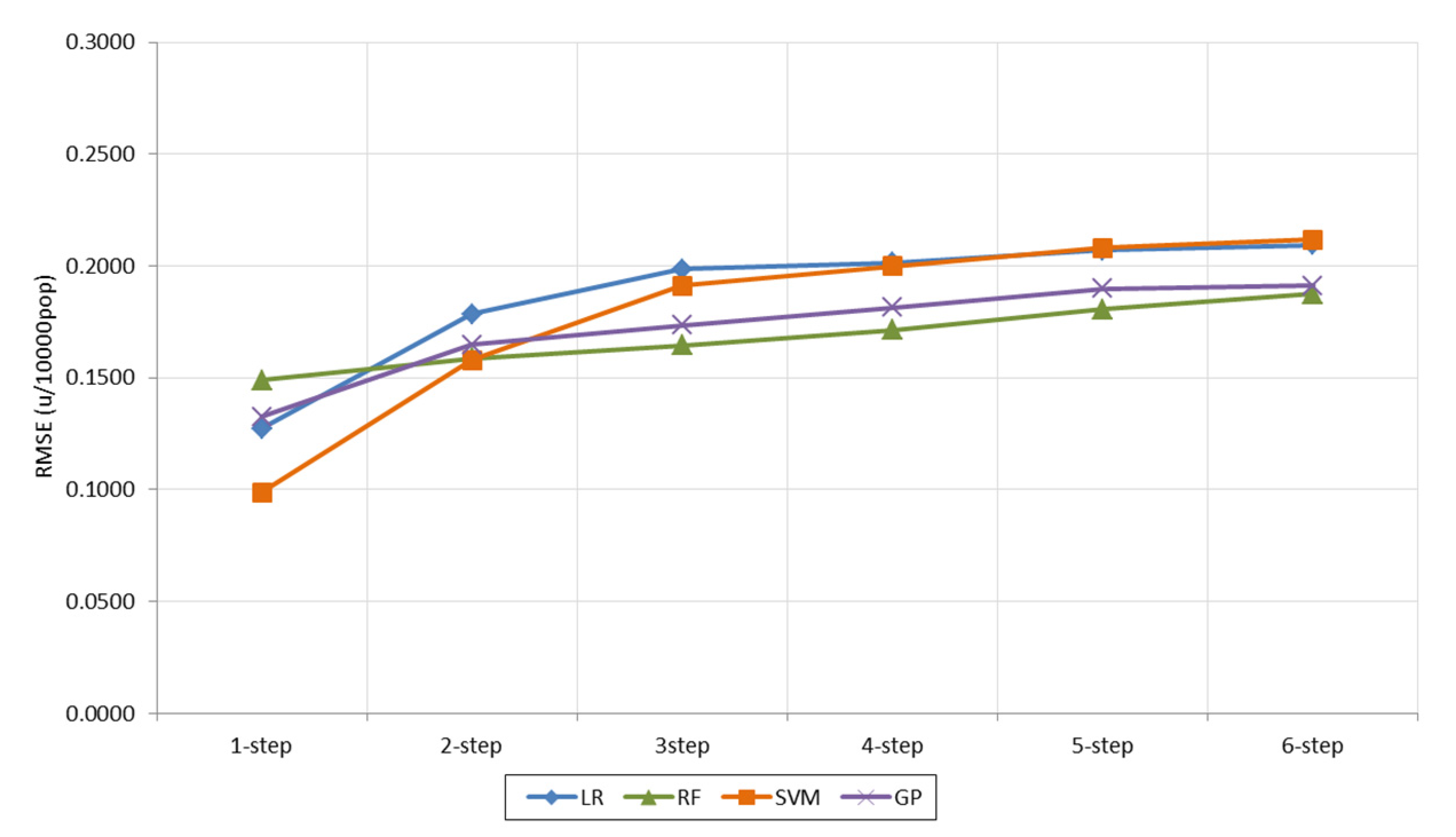
5.6. Data Modeling and Forecasting
- -
- Linear Regression (LR).
- -
- Support Vector Machines (SVM).
- -
- Random Forest (RF).
- -
- Gaussian Process (GP).
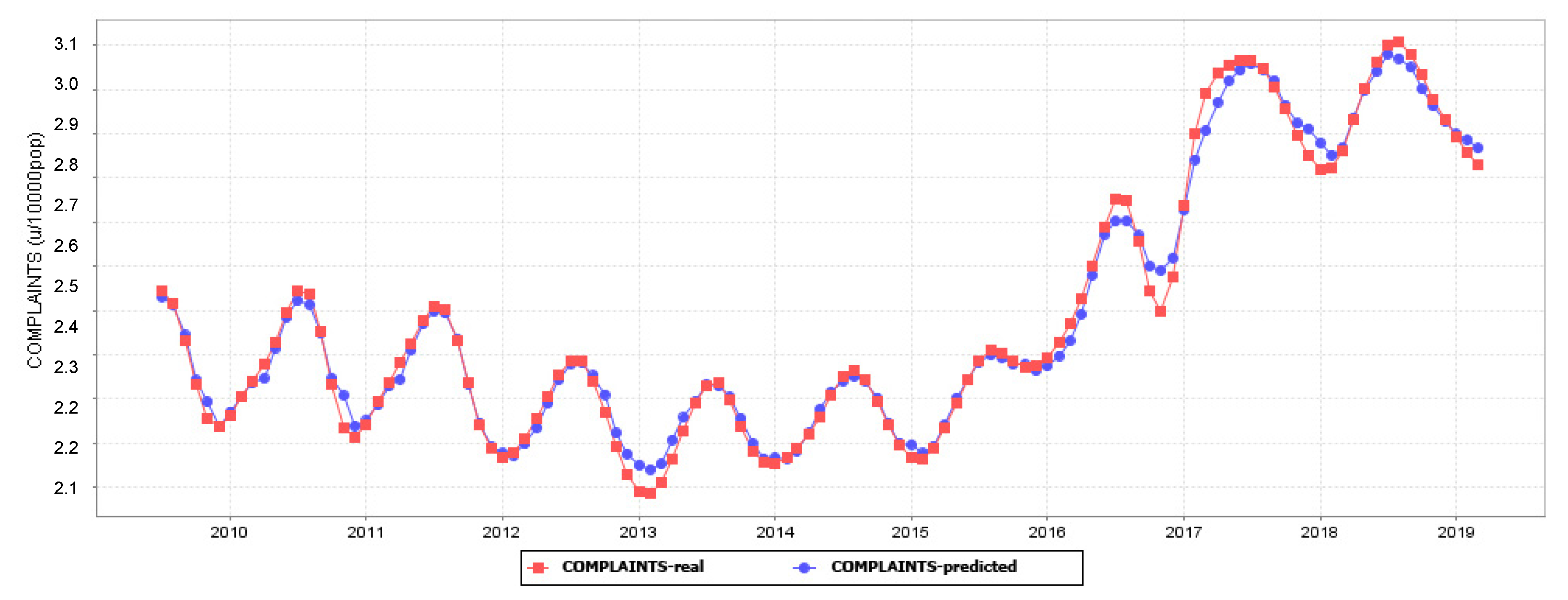
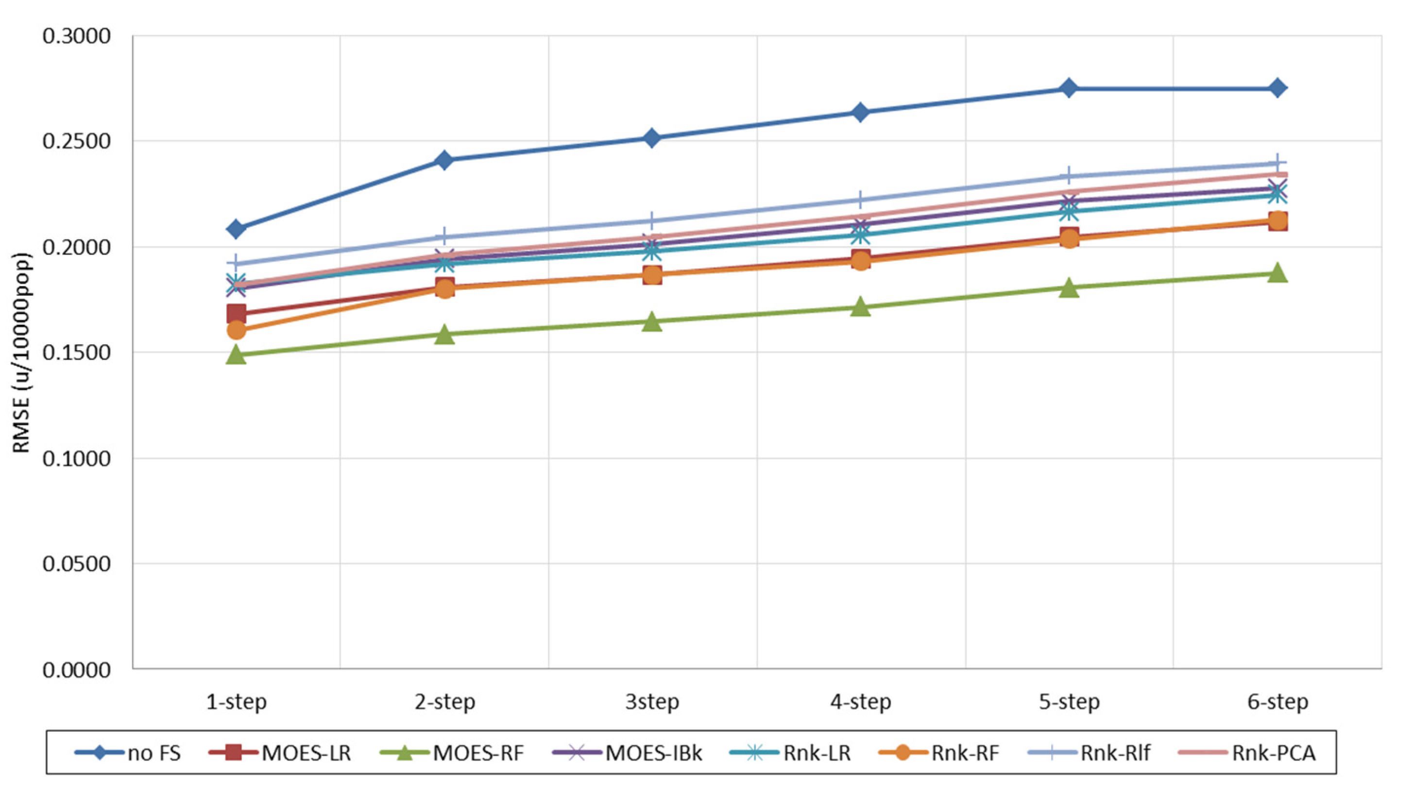
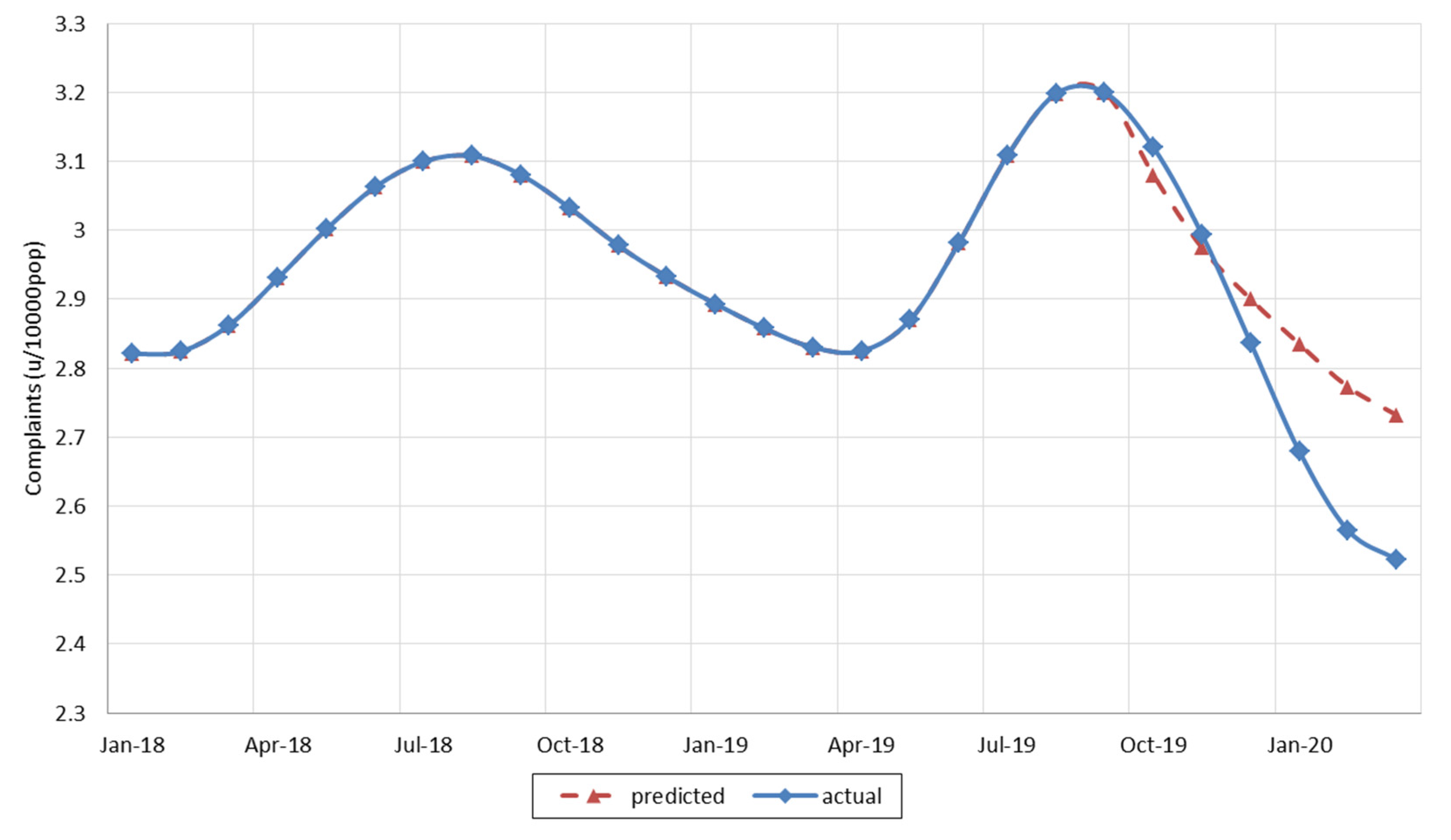
6. Results and Discussion: Forecasting Performance
7. Conclusions and Future Works
Author Contributions
Funding
Acknowledgments
Conflicts of Interest
References
- Devries, K.M.; Mak, J.Y.; Garcia-Moreno, C.; Petzold, M.; Child, J.C.; Falder, G.; Pallitto, C. The global prevalence of intimate partner violence against women. Science 2013, 340, 1527–1528. [Google Scholar] [CrossRef] [PubMed]
- Hyman, I.; Forte, T.; Mont, J.D.; Romans, S.; Cohen, M.M. Help-seeking rates for intimate partner violence (IPV) among Canadian immigrant women. Health Care Women Int. 2006, 27, 682–694. [Google Scholar] [CrossRef] [PubMed]
- Haraway, D. A manifesto for cyborgs: Science, technology, and socialist feminism in the 1980s. In Feminism/Postmodernism; Routledge: New York, NY, USA, 1990; pp. 190–233. [Google Scholar]
- Rodríguez-Rodríguez, I.; Rodríguez, J.V.; Elizondo-Moreno, A.; Heras-González, P.; Gentili, M. Towards a Holistic ICT Platform for Protecting Intimate Partner Violence Survivors Based on the IoT Paradigm. Symmetry 2020, 12, 37. [Google Scholar] [CrossRef]
- Rodríguez-Rodríguez, I.; Zamora-Izquierdo, M.Á.; Rodríguez, J.V. Towards an ICT-based platform for type 1 diabetes mellitus management. Appl. Sci. 2018, 8, 511. [Google Scholar] [CrossRef]
- Bryant, R.; Katz, R.H.; Lazowska, E.D. Big-data Computing: Creating Revolutionary Breakthroughs in Commerce, Science and Society. In Computing ResearchInitiatives for the 21st Century, Computing Research Association; Version 8; Washington, DC, USA, 2008; Available online: http://www.cra.org/ccc/docs/init/Big_Data.pdf (accessed on 11 August 2020).
- Islam, A.; Akter, A.; Hossain, B.A. HomeGuard: A Smart System to Deal with the Emergency Response of Domestic Violence Victims. arXiv 2018, arXiv:1803.09401. [Google Scholar]
- Hegde, N.; Bries, M.; Swibas, T.; Melanson, E.; Sazonov, E. Automatic recognition of activities of daily living utilizing insole-based and wrist-worn wearable sensors. IEEE J. Biomed. Health Inform. 2017, 22, 979–988. [Google Scholar] [CrossRef]
- Glaeser, E.L.; Hillis, A.; Kominers, S.D.; Luca, M. Crowdsourcing city government: Using tournaments to improve inspection accuracy. Am. Econ. Rev. 2016, 106, 114–118. [Google Scholar] [CrossRef]
- Cranmer, S.J.; Desmarais, B.A. What Can We Learn from Predictive Modeling? Political Anal. 2017, 25, 145–166. [Google Scholar] [CrossRef]
- Molina, M.; Garip, F. Machine learning for sociology. Ann. Rev. Sociol. 2019, 45, 27–45. [Google Scholar] [CrossRef]
- Kleinberg, J.; Ludwig, J.; Mullainathan, S.; Obermeyer, Z. Prediction policy problems. Am. Econ. Rev. 2015, 105, 491–495. [Google Scholar] [CrossRef]
- Cederman, L.E.; Weidmann, N.B. Predicting armed conflict: Time to adjust our expectations? Science 2017, 355, 474–476. [Google Scholar] [CrossRef] [PubMed]
- Beck, N.; King, G.; Zeng, L. Improving quantitative studies of international conflict: A conjecture. Am. Political Sci. Rev. 2000, 94, 21–35. [Google Scholar] [CrossRef]
- Brandt, P.T.; Freeman, J.R.; Schrodt, P.A. Real time, time series forecasting of inter-and intra-state political conflict. Confl. Manag. Peace Sci. 2011, 28, 41–64. [Google Scholar] [CrossRef]
- Perry, C. Machine learning and conflict prediction: A use case. Stab. Int. J. Secur. Dev. 2013, 2, 56. [Google Scholar]
- Kleinberg, J.; Liang, A.; Mullainathan, S. The Theory is Predictive, But is it Complete? An Application to Human Perception of Randomness. In Proceedings of the 2017 ACM Conference on Economics and Computation, Cambridge, MA, USA, 26–30 June 2017; pp. 125–126. [Google Scholar]
- Coglianese, C.; Lehr, D. Regulating by robot: Administrative decision making in the machine-learning era. Geo LJ 2016, 105, 1147. [Google Scholar]
- Lawrenz, F.; Lembo, J.F.; Schade, T. Time series analysis of the effect of a domestic violence directive on the number of arrests per day. J. Crim. Justice 1988, 16, 493–498. [Google Scholar] [CrossRef]
- Ozkan, T. Predicting Recidivism through Machine Learning. Doctoral Dissertation, University of Texas, Dallas, TX, USA, 2017. [Google Scholar]
- Ward-Lasher, A.; Sheridan, D.J.; Glass, N.E.; Messing, J.T. Prediction of Interpersonal Violence: An Introduction. Assess. Danger. 2017, 1, 1–23. [Google Scholar]
- Berk, R.A.; Sorenson, S.B.; Barnes, G. Forecasting domestic violence: A machine learning approach to help inform arraignment decisions. J. Empir. Leg. Stud. 2016, 13, 94–115. [Google Scholar] [CrossRef]
- Holcomb, J.P.; Sharpe, N.R. Forecasting police calls during peak times for the city of Cleveland. Case Stud. Bus. Ind. Gov. Stat. 2006, 1, 47–53. [Google Scholar]
- Sherman, L.W. Policing domestic violence 1967–2017. Criminol. Public Policy 2018, 17, 453–465. [Google Scholar] [CrossRef]
- Cohn, E.G. The prediction of police calls for service: The influence of weather and temporal variables on rape and domestic violence. J. Environ. Psychol. 1993, 13, 71–83. [Google Scholar] [CrossRef]
- Goodman, L.A.; Smyth, K.F.; Borges, A.M.; Singer, R. When crises collide: How intimate partner violence and poverty intersect to shape women’s mental health and coping? Trauma Violence Abus. 2009, 10, 306–329. [Google Scholar] [CrossRef]
- Hilton, N.Z.; Eke, A.W. Assessing risk of intimate partner violence. Assess. Danger. 2017, 207, 139–178. [Google Scholar]
- Heras-González, P.; Nardi-Rodríguez, A. Respuesta institucional a la Violencia de Género en la Comunidad Valenciana (España). Institutional response to Gender-based Violence in the Valencian Community (Spain). General. Valencia. Serv. Publ. 2020, 1, 1–30. [Google Scholar]
- Thornton, S. Police Attempts to Predict Domestic Murder and Serious Assaults: Is Early Warning Possible Yet? Camb. J. Evid.-Based Policy 2017, 1, 64–80. [Google Scholar] [CrossRef]
- Chalkley, R.; Strang, H. Predicting domestic homicides and serious violence in Dorset: A replication of Thornton’s Thames Valley analysis. Camb. J. Evid.-Based Policy 2017, 1, 81–92. [Google Scholar] [CrossRef]
- Delgadillo-Aleman, S.; Ku-Carrillo, R.; Perez-Amezcua, B.; Chen-Charpentier, B. A mathematical model for intimate partner violence. Math. Comput. Appl. 2019, 24, 29. [Google Scholar] [CrossRef]
- Poza, E.; Jódar, L.U.C.A.S.; Barreda, S. Mathematical Modeling of Hidden Intimate Partner Violence in Spain: A Quantitative and Qualitative Approach. In Abstract and Applied Analysis; Hindawi: New York, NY, USA, 2016; Volume 2016. [Google Scholar]
- Guyon, I.; Elissee, A. An introduction to variable and feature selection. J. Mach. Learn. Res. 2003, 3, 1157–1182. [Google Scholar]
- Sheikhpour, R.; Sarram, M.A.; Gharaghani, S.; Chahooki MA, Z. A survey on semi-supervised feature selection methods. Pattern Recognit. 2017, 64, 141–158. [Google Scholar] [CrossRef]
- Hastie, T.; Tibshirani, R.; Tibshirani, R.J. Extended comparisons of best subset selection, forward stepwise selection, and the lasso. arXiv 2017, arXiv:1707.08692. [Google Scholar]
- Kohavi, R.; John, G.H. Wrappers for feature subset selection. Artif. Intell. 1997, 97, 273–324. [Google Scholar] [CrossRef]
- Karegowda, A.G.; Jayaram, M.A.; Manjunath, A.S. Feature subset selection problem using wrapper approach in supervised learning. Int. J. Comput. Appl. 2010, 1, 13–17. [Google Scholar] [CrossRef]
- Yang, K.; Yoon, H.; Shahabi, C. A supervised feature subset selection technique for multivariate time series. In Proceedings of the Workshop on Feature Selection for Data Mining: Interfacing Machine Learning with Statistics, New Port Beach, CA, USA, 23 April 2005; pp. 92–101. [Google Scholar]
- Crone, S.F.; Kourentzes, N. Feature selection for time series prediction—A combined filter and wrapper approach for neural networks. Neurocomputing 2010, 73, 1923–1936. [Google Scholar] [CrossRef]
- Sánchez-Maroño, N.; Alonso-Betanzos, A.; Tombilla-Sanromán, M. Filter Methods for Feature Selection—A Comparative Study. In International Conference on Intelligent Data Engineering and Automated Learning; Springer: Berlin/Heidelberg, Germany, 2007; pp. 178–187. [Google Scholar]
- Fonti, V.; Belitser, E. Feature selection using lasso. VU Amst. Res. Pap. Bus. Anal. 2017, 30, 1–25. [Google Scholar]
- Zhang, H.; Zhang, R.; Nie, F.; Li, X. A Generalized Uncorrelated Ridge Regression with Nonnegative Labels for Unsupervised Feature Selection. In Proceedings of the 2018 IEEE International Conference on Acoustics, Speech and Signal Processing (ICASSP), Calgary, AB, Canada, 15–20 April 2018; pp. 2781–2785. [Google Scholar]
- Zitzler, E.; Thiele, L. Multiobjective evolutionary algorithms: A comparative case study and the strength Pareto approach. IEEE Trans. Evol. Comput. 1999, 3, 257–271. [Google Scholar] [CrossRef]
- Bolón-Canedo, V.; Sánchez-Maroño, N.; Alonso-Betanzos, A. A review of feature selection methods on synthetic data. Knowl. Inf. Syst. 2013, 34, 483–519. [Google Scholar] [CrossRef]
- Bolón-Canedo, V.; Sánchez-Maroño, N.; Alonso-Betanzos, A. Distributed feature selection: An application to microarray data classification. Appl. Soft Comput. 2015, 30, 136–150. [Google Scholar] [CrossRef]
- Wolpert, D.H.; Macready, W.G. No free lunch theorems for optimization. IEEE Trans. Evol. Comput. 1997, 1, 67–82. [Google Scholar] [CrossRef]
- Brockwell, P.J.; Davis, R.A.; Calder, M.V. Introduction to Time Series and Forecasting; Springer: New York, NY, USA, 2002; Volume 2, pp. 3118–3121. [Google Scholar]
- Faloutsos, C.; Gasthaus, J.; Januschowski, T.; Wang, Y. Forecasting big time series: Old and new. Proc. Vldb Endow. 2018, 11, 2102–2105. [Google Scholar] [CrossRef]
- Kalekar, P.S. Time series forecasting using holt-winters exponential smoothing. Kanwal Rekhi Sch. Inf. Technol. 2004, 4329008, 1–13. [Google Scholar]
- Vapnik, V. The Nature of Statistical Learning Theory; Springer Science & Business Media: Berlin, Germany, 2013. [Google Scholar]
- Schölkopf, B.; Smola, A.J. A Short Introduction to Learning with Kernels. In Advanced Lectures on Machine Learning; Springer: Berlin/Heidelberg, Germany, 2003; pp. 41–64. [Google Scholar]
- Kuhn, M.; Johnson, K. Applied Predictive Modeling; Springer: New York, NY, USA, 2002; Volume 26. [Google Scholar]
- Breiman, L. Bagging predictors. Mach. Learn. 1996, 24, 123–140. [Google Scholar] [CrossRef]
- Liaw, A.; Wiener, M. Classification and regression by randomForest. R News 2002, 2, 18–22. [Google Scholar]
- Oshiro, T.M.; Perez, P.S.; Baranauskas, J.A. How Many Trees in A Random Forest? In International Workshop on Machine Learning and Data Mining in Pattern Recognition; Springer: Berlin/Heidelberg, Germany, 2012; pp. 154–168. [Google Scholar]
- Williams, C.K.; Barber, D. Bayesian classification with gaussian processes. IEEE Trans. Pattern Anal. Mach. Intell. 1998, 20, 1342–1351. [Google Scholar] [CrossRef]
- Ortmann, L.; Shi, D.; Dassau, E.; Doyle, F.J.; Leonhardt, S.; Misgeld, B.J. Gaussian process-based model predictive control of blood glucose for patients with type 1 diabetes mellitus. In Proceedings of the 2017 11th Asian Control Conference (ASCC), Gold Coast, QLD, Australia, 17–20 December 2017. [Google Scholar]
- Williams, C.K.; Rasmussen, C.E. Gaussian Processes for Machine Learning; MIT Press: Cambridge, MA, USA, 2006; Volume 2, p. 4. [Google Scholar]
- Landau, S.F.; Fridman, D. The seasonality of violent crime: The case of robbery and homicide in Israel. J. Res. Crime Delinq. 1993, 30, 163–191. [Google Scholar] [CrossRef]
- Bowlus, A.J.; Seitz, S. Domestic violence, employment, and divorce. Int. Econ. Rev. 2006, 47, 1113–1149. [Google Scholar] [CrossRef]
- Anderberg, D.; Rainer, H.; Wadsworth, J.; Wilson, T. Unemployment and domestic violence: Theory and evidence. Econ. J. 2016, 126, 1947–1979. [Google Scholar] [CrossRef]
- Brahmapurkar, K.P. Gender equality in India hit by illiteracy, child marriages and violence: A hurdle for sustainable development. Pan Afr. Med. J. 2017, 28, 178. [Google Scholar] [CrossRef]
- Hussain, S.; Dahan, N.A.; Ba-Alwib, F.M.; Ribata, N. Educational data mining and analysis of students’ academic performance using WEKA. Indones. J. Electr. Eng. Comput. Sci. 2018, 9, 447–459. [Google Scholar] [CrossRef]
- Kiranmai, S.A.; Laxmi, A.J. Data mining for classification of power quality problems using WEKA and the effect of attributes on classification accuracy. Prot. Control Mod. Power Syst. 2018, 3, 29. [Google Scholar] [CrossRef]
- Lang, S.; Bravo-Marquez, F.; Beckham, C.; Hall, M.; Frank, E. Wekadeeplearning4j: A deep learning package for weka based on deeplearning4j. Knowl.-Based Syst. 2019, 178, 48–50. [Google Scholar] [CrossRef]
- Jiménez, F.; Sánchez, G.; García, J.M.; Sciavicco, G.; Miralles, L. Multi-objective evolutionary feature selection for online sales forecasting. Neurocomputing 2017, 234, 75–92. [Google Scholar] [CrossRef]
- Novaković, J. Toward optimal feature selection using ranking methods and classification algorithms. Yugoslav J. Oper. Res. 2016, 21, 119–135. [Google Scholar] [CrossRef]
- Nicodemus, K.K. Letter to the editor: On the stability and ranking of predictors from random forest variable importance measures. Brief. Bioinform. 2011, 12, 369–373. [Google Scholar] [CrossRef] [PubMed]
- Aha, D.W.; Kibler, D.; Albert, M.K. Instance-based learning algorithms. Mach. Learn. 1991, 6, 37–66. [Google Scholar] [CrossRef]
- Kononenko, I. (1994, April). Estimating Attributes: Analysis and Extensions of RELIEF. In European Conference on Machine Learning; Springer: Berlin/Heidelberg, Germany, 1994; pp. 171–182. [Google Scholar]
- Abdi, H.; Williams, L.J. Principal component analysis. Wiley Interdiscip. Rev. Comput. Stat. 2010, 2, 433–459. [Google Scholar] [CrossRef]
- Bergmeir, C.; Benítez, J.M. On the use of cross-validation for time series predictor evaluation. Inf. Sci. 2012, 191, 192–213. [Google Scholar] [CrossRef]


| Variable | Description | Units |
|---|---|---|
| PROVINCE | Spanish province under study (or the whole country) | (Categorical) |
| DATE | Data collection date | Month |
| QUARTER | Quarter of the year | Quarter |
| YEAR | Year of data collection | Year |
| POP_TOT | Total population of the province | Units |
| RATIO_MvsW | Ratio Population of men/women | Adimensional |
| MARRIAGES | Number of new weddings | Units/10,000 pop |
| SEPARATIONS | Number of separated marriages | Units/100,000 pop |
| BIRTHS | Number of newborn children | Units/1000 pop |
| CALLS | Calls to special telephone number 016 (requests for information and assistance) | Units/10,000 pop |
| COMPLAINTS | Complaints made to a Court | Units/10,000 pop |
| DEVICES | Security devices for tracking offenders | Units/100,000 pop |
| PROTECTION_ORDER | Restraining order for survivors decreed by a judge | Units/10,000 pop |
| RISK_UN | Survivors with unappreciated risk after police valuation | Units/10,000 pop |
| RISK_L | Survivors with low risk after police valuation | Units/10,000 pop |
| RISK_M | Survivors with medium risk after police valuation | Units/10,000 pop |
| RISK_H | Survivors with high risk after police valuation | Units/10,000 pop |
| RISK_EH | Survivors with extremely high risk after police valuation | Units/10,000 pop |
| FATALITIES | Murdered victims of GBV | Units/1,000,000 pop |
| GDP | Gross Domestic Product per capita | €/10,000 pop |
| EMPL_MEN | Employed men | Units/100 pop |
| UNEMPL_MEN | Unemployed women | Units/100 pop |
| INACT_MEN | Inactive women | Units/100 pop |
| EMPL_WOM | Employed women | Units/100 pop |
| UNEMPL_WOM | Unemployed women | Units/100 pop |
| INACT_WOM | Inactive women | Units/100 pop |
| ILLIT_MEN | Illiterate men | Units/100 pop |
| ILLIT_WOM | Illiterate women | Units/100 pop |
| PRIM_ED_MEN | Primary education men | Units/100 pop |
| SEC_ED_MEN | Secondary education men | Units/100 pop |
| HIGH_ED_MEN | Higher education men | Units/100 pop |
| PRIM_ED_WOM | Primary education women | Units/100 pop |
| SEC_ED_WOM | Secondary education women | Units/100 pop |
| HIGH_ED_WOM | Higher education women | Units/100 pop |
| Search Method | Attribute Evaluator | Predictor | Acronym |
|---|---|---|---|
| MOES | Wrapper | Linear Regression | MOES-LR |
| Random Forest | MOES-RF | ||
| IBk | MOES-IBk | ||
| Ranker | Wrapper (Classifier) | Linear Regression | Rnk-LR |
| Random Forest | Rnk-RF | ||
| Filter | Relief | Rnk-Rlf | |
| PCA | Rnk-PCA |
| Technique | Command |
|---|---|
| MOES | weka.attributeSelection.MultiObjectiveEvolutionarySearch -generations 20 -population-size 100 -seed 1 -algorithm 0 -report-frequency 20 -log-file “C:\\Program Files\\Weka-3-8” |
| Ranker | weka.attributeSelection. Ranker -T -1. 8 -N -1 |
| Wrapper LR | weka.attributeSelection.WrapperSubsetEval -B weka.classifiers.functions.LinearRegression -F 5 -T 0.01 -R 1 -E RMSE -- -S 0 -R 1.0E-8 -num-decimal-places 4 |
| Wrapper RF | weka.attributeSelection.WrapperSubsetEval -B weka.classifiers.trees.RandomForest -F 5 -T 0.01 -R 1 -E RMSE -- -P 100 -I 100 -num-slots 1 -K 0 -M 1.0 -V 0.001 -S 1 -num-decimal-places 4 |
| Wrapper IBk | weka.attributeSelection.WrapperSubsetEval -B weka.classifiers.lazy.IBk -F 5 -T 0.01 -R 1 -E RMSE -- -K 1 -W 0 -A “weka.core.neighboursearch.LinearNNSearch -A \”weka.core.EuclideanDistance -R first-last\”“ -num-decimal-places 4 |
| Classifier LR | weka.attributeSelection.ClassifierAttributeEval -execution-slots 1 -B weka.classifiers.functions.LinearRegression -F 5 -T 0.01 -R 1 -E RMSE -- -S 0 -R 1.0E-8 -num-decimal-places 4 |
| Classifier RF | weka.attributeSelection.ClassifierAttributeEval -execution-slots 1 -B weka.classifiers.trees.RandomForest -F 5 -T 0.01 -R 1 -E RMSE -- -P 100 -I 100 -num-slots 1 -K 0 -M 1.0 -V 0.001 -S 1 -num-decimal-places 4 |
| Relief | weka.attributeSelection.ReliefFAttributeEval -M -1 -D 1 -K 10 |
| PCA | weka.attributeSelection.PrincipalComponents -R 0.95 -A 5 |
| Technique | Command |
|---|---|
| LR | weka.classifiers.functions.LinearRegression -S 0 -R 1.0E-8 -num-decimal-places 4 |
| RF | weka.classifiers.trees.RandomForest -P 100 -I 100 -num-slots 1 -K 0 -M 1.0 -V 0.001 -S 1 |
| SVM | weka.classifiers.functions.SMOreg -C 1.0 -N 0 -I “weka.classifiers.functions.supportVector.RegSMOImproved -T 0.001 -V -P 1.0E-12 -L 0.001 -W 1” -K “weka.classifiers.functions.supportVector.PolyKernel -E 1.0 -C 250007” |
| GP | weka.classifiers.functions.GaussianProcesses -L 1.0 -N 0 -K “weka.classifiers.functions.supportVector.PolyKernel -E 1.0 -C 250007” -S 1 |
| RMSE | ||||||||
|---|---|---|---|---|---|---|---|---|
| Subset FS | 1 Step | 2 Step | 3 Step | 4 Step | 5 Step | 6 Step | Standard Deviation | |
| Forecasting technique: LR | ||||||||
| No F.S. | 0.2309 | 0.4502 | 0.6627 | 0.8719 | 1.0802 | 1.2785 | 0.7624 | 0.3922 |
| MOES-LR | 0.2229 | 0.2784 | 0.2938 | 0.3059 | 0.3224 | 0.3418 | 0.2942 | 0.0413 |
| MOES-RF | 0.1273 | 0.1784 | 0.1985 | 0.2015 | 0.2069 | 0.2093 | 0.1870 | 0.0312 |
| MOES-IBk | 0.0914 | 0.1878 | 0.2853 | 0.3761 | 0.4576 | 0.5227 | 0.3202 | 0.1638 |
| Rnk-LR | 0.1033 | 0.2034 | 0.2932 | 0.3589 | 0.4012 | 0.4039 | 0.2940 | 0.1203 |
| Rnk-RF | 0.1198 | 0.2058 | 0.2632 | 0.3014 | 0.3292 | 0.3493 | 0.2615 | 0.0861 |
| Rnk-Rlf | 0.3860 | 0.4017 | 0.4195 | 0.4362 | 0.4442 | 0.4253 | 0.4188 | 0.0217 |
| Rnk-PCA | 0.2289 | 0.3227 | 0.3619 | 0.3859 | 0.4081 | 0.4315 | 0.3565 | 0.0729 |
| 0.3618 | ||||||||
| Forecasting technique: RF | ||||||||
| No F.S. | 0.2083 | 0.2407 | 0.2513 | 0.2635 | 0.2748 | 0.2747 | 0.2522 | 0.0253 |
| MOES-LR | 0.1680 | 0.1808 | 0.1867 | 0.1943 | 0.2047 | 0.2117 | 0.1910 | 0.0160 |
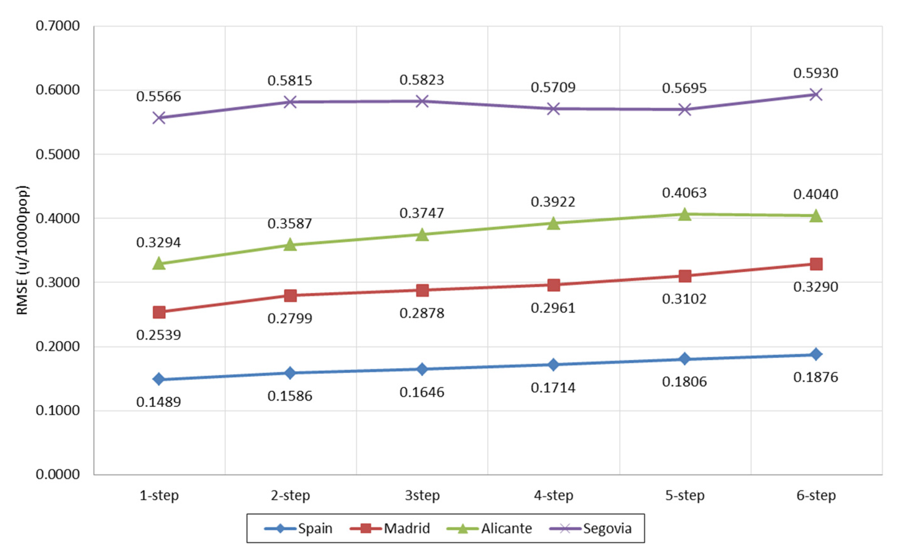
| MOES-RF | 0.1489 | 0.1586 | 0.1646 | 0.1714 | 0.1806 | 0.1876 | 0.1686 | 0.0143 |
| MOES-IBk | 0.1803 | 0.1941 | 0.2012 | 0.2104 | 0.2214 | 0.2275 | 0.2058 | 0.0176 |
| Rnk-LR | 0.1824 | 0.1919 | 0.1978 | 0.2055 | 0.2166 | 0.2246 | 0.2031 | 0.0157 |
| Rnk-RF | 0.1605 | 0.1801 | 0.1866 | 0.1930 | 0.2034 | 0.2125 | 0.1894 | 0.0183 |
| Rnk-Rlf | 0.1919 | 0.2047 | 0.2121 | 0.2219 | 0.2333 | 0.2395 | 0.2172 | 0.0179 |
| Rnk-PCA | 0.1820 | 0.1960 | 0.2047 | 0.2144 | 0.2258 | 0.2343 | 0.2095 | 0.0193 |
| 0.2046 | ||||||||
| Forecasting technique: SVM | ||||||||
| No F.S. | 0.3825 | 0.4632 | 0.4879 | 0.5067 | 0.5307 | 0.5600 | 0.4885 | 0.0618 |
| MOES-LR | 0.1706 | 0.2204 | 0.2372 | 0.2489 | 0.2621 | 0.2722 | 0.2352 | 0.0365 |
| MOES-RF | 0.0987 | 0.1580 | 0.1913 | 0.1999 | 0.2082 | 0.2118 | 0.1780 | 0.0434 |
| MOES-IBk | 0.1782 | 0.2765 | 0.3288 | 0.3603 | 0.3838 | 0.4056 | 0.3222 | 0.0837 |
| Rnk-LR | 0.0759 | 0.1420 | 0.1929 | 0.2198 | 0.2314 | 0.2292 | 0.1819 | 0.0618 |
| Rnk-RF | 0.1320 | 0.1648 | 0.1850 | 0.1922 | 0.1997 | 0.1997 | 0.1789 | 0.0264 |
| Rnk-Rlf | 0.1292 | 0.2462 | 0.3460 | 0.4273 | 0.4974 | 0.5583 | 0.3674 | 0.1605 |
| Rnk-PCA | 0.1321 | 0.2579 | 0.3762 | 0.4865 | 0.5869 | 0.6711 | 0.4185 | 0.2032 |
| 0.2963 | ||||||||
| Forecasting technique: GP | ||||||||
| No F.S. | 0.3402 | 0.3823 | 0.3922 | 0.4005 | 0.4156 | 0.4383 | 0.3949 | 0.0332 |
| MOES-LR | 0.1540 | 0.2160 | 0.2325 | 0.2344 | 0.2403 | 0.2531 | 0.2217 | 0.0353 |
| MOES-RF | 0.1325 | 0.1648 | 0.1735 | 0.1813 | 0.1898 | 0.1913 | 0.1722 | 0.0219 |
| MOES-IBk | 0.1694 | 0.2171 | 0.2325 | 0.2443 | 0.2560 | 0.2611 | 0.2301 | 0.0337 |
| Rnk-LR | 0.1513 | 0.2118 | 0.2317 | 0.2373 | 0.2469 | 0.2603 | 0.2232 | 0.0388 |
| Rnk-RF | 0.1720 | 0.2125 | 0.2220 | 0.2276 | 0.2374 | 0.2512 | 0.2205 | 0.0272 |
| Rnk-Rlf | 0.3075 | 0.3525 | 0.3649 | 0.3758 | 0.3927 | 0.4161 | 0.3683 | 0.0371 |
| Rnk-PCA | 0.2479 | 0.2989 | 0.3120 | 0.3229 | 0.3396 | 0.3592 | 0.3134 | 0.0384 |
| 0.2680 | ||||||||
| Subset FS | Spain | Madrid | Alicante | Segovia | ||||
|---|---|---|---|---|---|---|---|---|
| Standard Deviation | Standard Deviation | Standard Deviation | Standard Deviation | |||||
| Forecasting technique: LR | ||||||||
| No F.S. | 0.7624 | 0.3922 | 1.1144 | 0.5175 | 1.1849 | 0.2454 | 1.7304 | 0.5124 |
| MOES-LR | 0.2942 | 0.0413 | 0.3430 | 0.1167 | 0.4724 | 0.1636 | 0.5129 | 0.1208 |
| MOES-RF | 0.1870 | 0.0312 | 0.2709 | 0.0066 | 0.3974 | 0.0704 | 0.3104 | 0.1108 |
| MOES-IBk | 0.3202 | 0.1638 | 0.5108 | 0.2423 | 0.9960 | 0.3369 | 0.8974 | 0.1692 |
| Rnk-LR | 0.2940 | 0.1203 | 0.3519 | 0.1406 | 0.8525 | 0.0843 | 0.3370 | 0.0107 |
| Rnk-RF | 0.2615 | 0.0861 | 0.3153 | 0.0493 | 0.4081 | 0.0047 | 0.2756 | 0.1074 |
| Rnk-Rlf | 0.4188 | 0.0217 | 0.5127 | 0.1821 | 1.1618 | 0.3647 | 1.2120 | 0.1902 |
| Rnk-PCA | 0.3565 | 0.0729 | 0.6136 | 0.0748 | 1.0383 | 0.3725 | 1.1588 | 0.7191 |
| 0.3618 | 0.5041 | 0.8139 | 0.8043 | |||||
| Forecasting technique: RF | ||||||||
| No F.S. | 0.2522 | 0.0253 | 0.3198 | 0.0208 | 0.4245 | 0.0384 | 0.7339 | 0.0178 |
| MOES-LR | 0.1910 | 0.0160 | 0.3047 | 0.0224 | 0.3922 | 0.0360 | 0.6163 | 0.0118 |
| MOES-RF | 0.1686 | 0.0143 | 0.2928 | 0.0258 | 0.3776 | 0.0297 | 0.5756 | 0.0127 |
| MOES-IBk | 0.2058 | 0.0176 | 0.3051 | 0.0245 | 0.3978 | 0.0350 | 0.6592 | 0.0144 |
| Rnk-LR | 0.2031 | 0.0157 | 0.2990 | 0.0171 | 0.3804 | 0.0418 | 0.6195 | 0.0160 |
| Rnk-RF | 0.1894 | 0.0183 | 0.2921 | 0.0151 | 0.3704 | 0.0303 | 0.5798 | 0.0154 |
| Rnk-Rlf | 0.2172 | 0.0179 | 0.3158 | 0.0155 | 0.4026 | 0.0348 | 0.7262 | 0.0288 |
| Rnk-PCA | 0.2095 | 0.0193 | 0.3113 | 0.0218 | 0.4047 | 0.0324 | 0.6665 | 0.0231 |
| 0.2046 | 0.3051 | 0.3938 | 0.6471 | |||||
| Forecasting technique: SVM | ||||||||
| No F.S. | 0.4885 | 0.0618 | 0.8038 | 0.2394 | 1.4879 | 0.4664 | 1.7207 | 0.7698 |
| MOES-LR | 0.2352 | 0.0365 | 0.3276 | 0.1057 | 0.4940 | 0.0888 | 0.4714 | 0.0987 |
| MOES-RF | 0.1780 | 0.0434 | 0.2508 | 0.0329 | 0.3407 | 0.0620 | 0.3418 | 0.1222 |
| MOES-IBk | 0.3222 | 0.0837 | 0.4588 | 0.1980 | 0.5229 | 0.1560 | 0.5738 | 0.1021 |
| Rnk-LR | 0.1819 | 0.0618 | 0.4583 | 0.1478 | 0.4866 | 0.1523 | 0.5341 | 0.4749 |
| Rnk-RF | 0.1789 | 0.0264 | 0.2620 | 0.0866 | 0.2975 | 0.0681 | 0.4103 | 0.2492 |
| Rnk-Rlf | 0.3674 | 0.1605 | 0.5824 | 0.0747 | 0.8858 | 0.3994 | 1.0350 | 0.1614 |
| Rnk-PCA | 0.4185 | 0.2032 | 0.4866 | 0.1357 | 0.7613 | 0.0778 | 0.6652 | 0.3641 |
| 0.2963 | 0.4538 | 0.6596 | 0.7190 | |||||
| Forecasting technique: GP | ||||||||
| No F.S. | 0.3949 | 0.0332 | 0.4966 | 0.0806 | 0.6799 | 0.0794 | 0.5454 | 0.0686 |
| MOES-LR | 0.2217 | 0.0353 | 0.3650 | 0.0664 | 0.3271 | 0.0738 | 0.3644 | 0.0682 |
| MOES-RF | 0.1722 | 0.0219 | 0.3013 | 0.0318 | 0.2602 | 0.0377 | 0.3033 | 0.0376 |
| MOES-IBk | 0.2301 | 0.0337 | 0.3709 | 0.0353 | 0.5322 | 0.0766 | 0.3788 | 0.0513 |
| Rnk-LR | 0.2232 | 0.0388 | 0.3136 | 0.0378 | 0.3299 | 0.0442 | 0.3116 | 0.0321 |
| Rnk-RF | 0.2205 | 0.0272 | 0.2762 | 0.0541 | 0.3192 | 0.0493 | 0.2899 | 0.0384 |
| Rnk-Rlf | 0.3683 | 0.0371 | 0.4226 | 0.0426 | 0.6502 | 0.1130 | 0.4225 | 0.0826 |
| Rnk-PCA | 0.3134 | 0.0384 | 0.3945 | 0.0716 | 0.6471 | 0.0606 | 0.4656 | 0.0939 |
| 0.2680 | 0.3676 | 0.4682 | 0.3852 | |||||
| Average among techniques | 0.2826 | 0.4076 | 0.5839 | 0.6389 | ||||
Publisher’s Note: MDPI stays neutral with regard to jurisdictional claims in published maps and institutional affiliations. |
© 2020 by the authors. Licensee MDPI, Basel, Switzerland. This article is an open access article distributed under the terms and conditions of the Creative Commons Attribution (CC BY) license (http://creativecommons.org/licenses/by/4.0/).
Share and Cite
Rodríguez-Rodríguez, I.; Rodríguez, J.-V.; Pardo-Quiles, D.-J.; Heras-González, P.; Chatzigiannakis, I. Modeling and Forecasting Gender-Based Violence through Machine Learning Techniques. Appl. Sci. 2020, 10, 8244. https://doi.org/10.3390/app10228244
Rodríguez-Rodríguez I, Rodríguez J-V, Pardo-Quiles D-J, Heras-González P, Chatzigiannakis I. Modeling and Forecasting Gender-Based Violence through Machine Learning Techniques. Applied Sciences. 2020; 10(22):8244. https://doi.org/10.3390/app10228244
Chicago/Turabian StyleRodríguez-Rodríguez, Ignacio, José-Víctor Rodríguez, Domingo-Javier Pardo-Quiles, Purificación Heras-González, and Ioannis Chatzigiannakis. 2020. "Modeling and Forecasting Gender-Based Violence through Machine Learning Techniques" Applied Sciences 10, no. 22: 8244. https://doi.org/10.3390/app10228244
APA StyleRodríguez-Rodríguez, I., Rodríguez, J.-V., Pardo-Quiles, D.-J., Heras-González, P., & Chatzigiannakis, I. (2020). Modeling and Forecasting Gender-Based Violence through Machine Learning Techniques. Applied Sciences, 10(22), 8244. https://doi.org/10.3390/app10228244