Using Common Spatial Patterns to Select Relevant Pixels for Video Activity Recognition

Abstract

Video activity recognition, despite being an emerging task, has been the subject of important research due to the importance of its everyday applications. Video camera surveillance could benefit greatly from advances in this field. In the area of robotics, the tasks of autonomous navigation or social interaction could also take advantage of the knowledge extracted from live video recording. In this paper, a new approach for video action recognition is presented. The new technique consists of introducing a method, which is usually used in Brain Computer Interface (BCI) for electroencephalography (EEG) systems, and adapting it to this problem. After describing the technique, achieved results are shown and a comparison with another method is carried out to analyze the performance of our new approach.

1. Introduction

Video Activity Recognition aims to automatically analyze and interpret particular events within video sequences. In the last years action recognition has gained interest, thanks to the growth of multimedia files availability and due to the amount of tasks it is useful for.

Currently, multimedia information generates large volumes of data, and this increases the need of developing automatic or semi-automatic systems which allow the labelling of video actions with different applications. For example, video cameras record data from different environments in real-time, which is useful, for instance, in security matters.

Many different domains can take advantage from video activity recognition, such as video security, video retrieval, or human-computer interaction. There are many different situations where a system that warns about suspicious actions in real time is highly beneficial, and since the enormous growth that multimedia data has experienced in recent years makes manual tagging tedious and sometimes impractical, video recognition can be used to perform annotation and indexing of videos. Furthermore, it can be useful to generate interactive systems for social purposes or for entertainment industry.

Identifying human actions in videos is a complex task. It is more challenging than image recognition, where a single frame represents the whole scene. In video recognition, a frame of a video where someone appears walking could also be a frame of a sequence of someone running, more frames are needed to see what action is taking place. The complexity of this task comes from the high intra-class variability that exists between the instances. This intra-class variability is caused by different factors, such as the diversity among people both in their appearance and in the style of execution of the action, the movements of the camera, the environment, which is usually affected by changes in lighting, shadows or occlusions, the viewpoint and the distance of the subject from the camera, and other factors, such as differences in resolution. Human actions are associated with a spatial and a temporal component, both random, so the performance of the same action is never identical.

In this paper, taking as a basis the work of Reference [1], a new approach for video action recognition is presented, where Common Spatial Pattern (CSP) algorithm is used, a method which is normally used in Brain Computer Interface (BCI) for electroencephalography (EEG) systems [2]. CSP is a dimensionality reduction technique which consists of finding an optimum spatial filter to separate a multidimensional signal into two classes, maximizing the variance of one of them while minimizing the variance of the other. In our approach input videos are represented as frame sequences and the temporal sequence of each pixel is treated as a signal (channel) to feed the CSP. After CSP is applied, some signals descriptors are selected for classification purposes. In classical CSP applications, only the signal variances and Linear Discriminant Analysis (LDA) classifier [3] are used; in this research, variances, minimum, maximum, and interquartil range (IQR) are taken as descriptors, and LDA, K Nearest Neighbors (KNN) [4] and Random Forests (RF) [5] as classifiers.

The rest of the paper is organized as follows—First, in Section 2 some related works are mentioned in order to introduce the topic. In Section 3 a theoretical framework is presented to explain the proposed approach in detail. In Section 4 the experimental setup is presented, the used data-set and the different experimentation carried out are explained thoroughly. To conclude, in Section 5 the obtained results are shown and a comparison between our approach and another method is made.

2. Related Work

Different trends have been identified when it comes to video action recognition. Several approaches have been developed to deal with this problem along the years [6,7,8]. The existing techniques can be divided in four main groups: the identification of space-time interest points, the representation of action sequence as 3D spatio-temporal volume, the use of motion information and the use of deep learning to process sequences of frames.

Space-time interest points extracted from video have been widely used for action recognition. For instance, the authors of Reference [9] extract accumulated holistic features from clouds of interest points in order to use the global spatiotemporal distribution of interest points. This is followed by an automatic feature selection. Their model captures robust and smooth motions, where denser and more informative interest points are obtained. In Reference [10] a compact video representation is presented, using 3D Harris and 3D SIFT for feature extraction. K-means clustering is used to form a visual word codebook which is later classified by a Support Vector Machine (SVM) and a Naive Bayes classifiers. The authors of Reference [11] apply surround suppression together with local and temporal constraints to achieve a robust and selective STIP detection. A vocabulary of visual-words is built with a bag-of-video words (BoVW) model of local N-jet features and a Support Vector Machine (SVM) is used for classification.

In order to try to improve the activity recognition, RGB Depth (RGB-D) cameras are used (e.g., Microsoft Kinect, Intel RealSense), which are robust to illumination changes. The authors of Reference [12] extract random occupancy pattern (ROP) semi-local features from depth sequences captured by depth cameras. These features are encoded with a sparse coding approach. The training phase of the presented approach is fast, robust and it does not require careful parameter tuning. In Reference [13] both RGB and Depth Camera are used to extract motion features, generating a Salient Information Map. For each motion history image, a Complete Local Binary descriptor is computed, extracting sign, magnitude and center descriptors from the Salient Information Map. Canonical Correlation Analysis and dimensionality reduction are used to combine depth and RGB features. The classification is performed by a multiclass SVM.

Approaches which focus in motion information usually rely on optical flow or appearance. In Reference [14] the authors propose dense trajectories to describe videos. From each frame dense trajectories are extracted and a dense optical flow algorithm is used to track them. To encode this information, the authors introduce a descriptor based on motion boundary histograms. They improve their work in Reference [15] by taking into account camera motion, using SURF descriptors and dense optical flow to match feature points between frames. A human detector is also used to avoid inconsistent matches between human motion and camera motion. The authors of Reference [16] decompose visual motion into dominant and residual motions. Then, they propose a new motion descriptor based on differential motion scalar quantities: divergence, curl and shear; the DCS descriptor, which captures additional information on the local motion patterns. The VLAD coding technique is used.

Recently, deep models have gained interest due to the good results they have obtained for image recognition. They are able to learn multiple layers of features hierarchies and automatically build high-level representations of the raw input. For video action recognition, Convolutional Neural Network (CNN) has been the most used model, extracting frames from videos and automatically classifying them by sending them as input features for the network. However, this way, temporal information is ignored and only spatial features are learnt. In Reference [17] they propose a two-stream CNN, where both spatial and temporal information are incorporated. The input of the spatial network is composed by the frames extracted from videos, whereas that of the temporal network is formed by the dense optical flow. Then, these two CNNs are combined by late fusion. Recurrent Neural Networks (RNNs) have also been proven to be effective for video activity recognition, specially Long Short-Term Memory (LSTM) networks. The authors of Reference [18] propose the use of a CNN along with a deep bidirectional LSTM (DB-LSTM) network. First, they use pre-trained AlexNet to extract deep features from every sixth frame of the videos. Then, sequence information from the features of video frames are learnt by the DB-LSTM. In Reference [19] the authors present a two-steam attention based LSTM network, which focuses on the effective features and assigns different weights to the outputs of each deep feature maps. They also propose a correlation network layer to identify the information loss and adjust the parameters.

3. CSP-Based Approach

Similar to Reference [1], the use of CSP is the main idea of the presented approach, although this time the signals to be processed are composed by temporal sequences of pixel. In this section, the used algorithm is explained, as well as the approach that is being introduced.

The Common Spatial Pattern (CSP) algorithm [20], a mathematical technique applied in signal processing, has been widely used in Brain Computer Interface (BCI) applications for electroencephalography (EEG) systems [21,22,23]. Research has also been published applying CSP in the field of electrocardiography (ECG) [24], electromyography (EMG) [25,26] or even in astronomical images for planet detection [27]. CSP was presented as an extension of Principal Component Analysis (PCA) and it consists of finding an optimum spatial filter which reduces the dimensionality of the original signals. Considering just two different classes, a CSP filter maximizes the difference of the variances between the classes, maximizing the variance of filtered signals of EEG of one of the targets while minimizing the variance for the other.

It must be clarified that, although the CSP algorithm has been used mainly with EEG problems, in this paper a new application is presented, the use of CSP filters for feature extraction in the human action recognition task. In our approach, each video represents a trial and each pixel is treated as an EEG channel, so the videos are taken as time series where the pixels are the channels which change over time. This is an application outside the usual field of analysis of physiological signals, somehow justified by the successful use in astronomical image processing [27], but here it is extended to videos depicting actions.

The full process can be seen in Figure 1. The first step consists of selecting the most relevant pixels of the frame sequences, that will be used to feed the CSP. In order to select the most relevant pixels, those which have the biggest variance are chosen, that is, the pixels that change most in the frame sequence. Once the pixels are selected and, hence, the signals are formed, the CSP is computed in order to separate the classes according to their variance.

4. Experimental Setup

In this section the details of the experiments that have been carried out are explained. First, the database used is presented. Then, different modalities are introduced and, finally, the optical flow method is explained, which has been used to make a comparison with the CSP approach. In Figure 2 a graphical overview of the presented approach is shown.

HMDB51 http://serre-lab.clps.brown.edu/resource/hmdb-a-large-human-motion-database [28] is an action recognition database which collects videos from various sources, mainly from movies but also from public databases such as YouTube, Google and Prelinger Archives. It consists of 6849 videos with 51 action categories and a minimum of 101 clips belong to each category. The action categories can be divided into 5 main groups:

• General facial actions: smiling, laughing, chewing, talking.
• Facial actions with object manipulation: smoking, eating, drinking.
• General body movements: cartwheeling, clapping hands, climbing, going up stairs, diving, falling down, backhand flipping, handstanding, jumping, pull-ups, push-ups, running, sitting down, sitting up, somersaulting, standing up, turning, walking, waving.
• Body movements with object interaction: brushing hair, catching, drawing a sword, dribbling, playing golf, hitting something, kicking a ball, picking something, pouring, pushing something, riding a bike, riding a horse, shooting a ball, shooting a bow, shooting a gun, swinging a baseball bat, drawing sword, throwing.
• Body movements for human interaction: fencing, hugging, kicking someone, kissing, punching, shaking hands, sword fighting.

Apart from the action label, other meta-labels are indicated in each clip. Those labels provide information about some features describing properties of the clip, such as camera motion, lighting conditions, or background. As some videos are taken from movies or YouTube, the variation of features is high and that extra information can be useful. The quality of the videos has also been measured (good, medium, bad), and they are rated depending on whether body parts vanish while the action is executed or not. It is worth mentioning that this extra information has not been used in this paper.

For our experiments only 6 classes have been selected due to the large amount of images. The selected classes are brushing hair, cartwheeling, fencing, punching, smoking and walking. To work with videos, their frames have been extracted in the first place. It has been decided to extract the same number of frames in every video of each class, so the largest video has been selected and the number of frames of the videos of that class is defined by it (in order not to cut any video and maybe lose the action performance). In

Table 1. Data-set class details.

	Videos	Frames/Video	Frames/Class
Brush hair	107	648	69,336
Fencing	116	301	34,916
Walk	282	534	150,588
Punch	126	502	63,252
Smoke	109	445	48,505
Cartwheel	103	132	13,596

the number of videos and number of frames are indicated for each class. In the case of HMDB51 as the number and length of the videos vary a lot, the number of frames changes in each class. However, the process to get the frames is the same, first the largest video is selected and it is used to determine the number of frames for the class. As some videos need to be extended to get the determined length, some of the frames of these videos are repeated.

Due to the difference between the number of videos of some of the classes, it has been decided to use the same amount of videos for both classes when performing the classification. The class with fewer instances indicates the number of videos in each of the experiments. For instance, when performing the classification between fencing (116) and smoke (109) 109 videos are used from each class, with a total of 218 videos. Since the class with the fewest instances has 103 videos, it was decided that it is a sufficient amount of instances to do the tests without having to apply any other more complicated balancing method.

It must also be mentioned that in order to perform all the introduced experiments, the size of the images is set to 25 × 25 due to the computational requirements of CSP. Moreover, the used CSP method is implemented to work with just 2 classes, therefore all the tests have been carried out using pairs of classes, one versus one [29].

4.1. Experiments

In this section the performed experiments are presented. They were developed using the technique introduced in Section 3, where the main idea is to consider the temporal sequence of pixel $i,j$ as a signal to be fed to the CSP. Taking that algorithm as a basis, different methods have been computed to make a comparison between them and see which one performs better.

Modalities

CSP algorithm was used in several modalities. The main change between the performed tests consists of deciding which pixels of the image are used to make the signals (channels) to calculate the CSP.

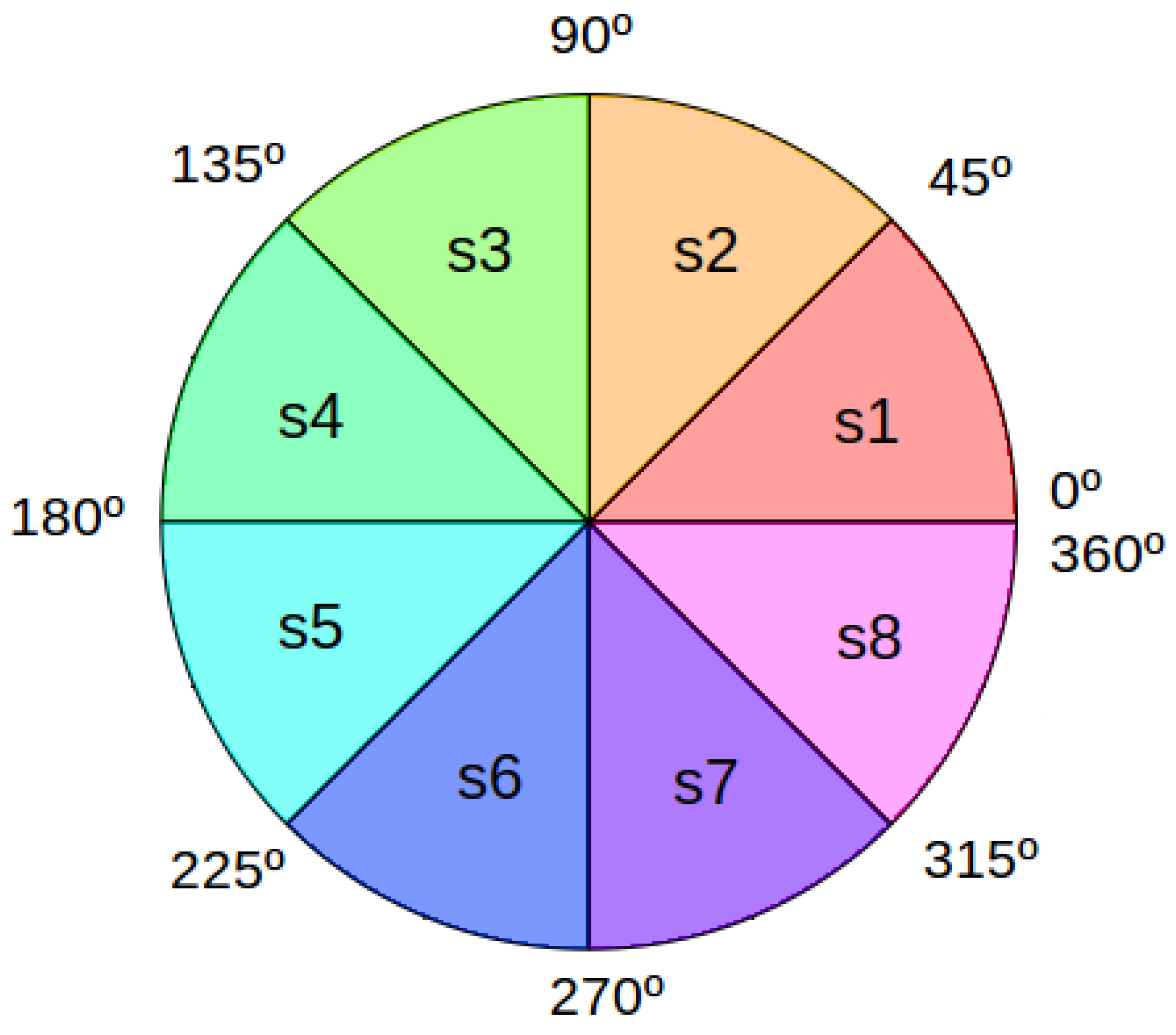
• Separation in quadrants.
  Taking into account that different actions have to be recognized, where in the video they occur should be taken into account, that is, in which area of the window. In many of the sequences used, the camera is static and the individuals performing the interaction appear almost centered. In these cases, it can be supposed that if the action they are performing is, for instance, smoke, it will be happening at the top of the images, while if the action is kick, it will be happening at the bottom part. In order to consider this approach, it was decided to divide each frame of the video in 16 quadrants as can be seen in Figure 3, and perform the whole classification pipeline for every one of them. Thus, each classifier focuses on an exact area of the videos. The final prediction is the result of the majority voting of these 16 classifiers.
• Pixels with maximum variance.
  CSP works with the variance of each channel. In some of the video sequences some objects from the scene, such as the background, are static, and do not change over time. The pixels corresponding to these static areas will produce a zero (or near zero, due to random fluctuations in pixel intensity) variance. This, apart from not providing useful information, can cause some problems at the time of executing the algorithm due to the calculation of the logarithm of the variances in the computation of CSP, yielding negative infinite values. In this case, it was decided to first select a group of pixels to extract the features, these are the pixels that change the most over time and therefore have the maximum variances. The hypothesis here is that they are the best candidates to represent the performed action. To select these pixels, the frames were transformed to grayscale, in order to have just one channel when calculating the variance of each pixel. In Figure 4 an example can be seen, where the 25 most relevant pixels have been selected for each quadrant.

Once the relevant pixels are selected and the quadrant separation has been decided, the classification is performed using different features extracted after the CSP filter. The main focus of the experimentation is the use of the variances of the signals after applying the Common Spatial Pattern filter. However, apart from the variances, many other information can be extracted from these transformed signals. Hence, some experiments are performed with just the information of the variances and other experiments also with information about the maximum and minimum values of the signal and the interquartile range ($IQR=Q3-Q1$). This information may be useful when performing the classification, and a comparison has been made between the results obtained by these two ways of performance:

• var
• var, min, max, IQR taken together

4.2. Optical Flow

A comparison between the use of optical flow vectors and CSP features has been made, in order to analyze which features provide the best information about the action of the videos.

There are some algorithms which compute the optical flow. In this paper the OpenCV implementation of Gunnar Farneback’s algorithm [30] is used. It provides a dense optical flow, which means that it calculates the optical flow for every point of the image. Dense techniques are slower but can be more accurate than sparse ones, which only compute the optical flow for some points of interest of the image. The result of Farneback’s method is a two dimensional array containing the vectors which represent the displacement of each point of the scene.

After having calculated the optical flow for every pixel, the vectors are divided into 10 bins and, according to the gradient direction of each pixel, a histogram is created. To create the histogram, the directions are separated in 8 stripes as can be seen in Figure 5. The features that are then trained are taken from this information.

Once the features for each video have been obtained, the classification is performed.

5. Experimental Results

After explaining how the process has been defined, the experimental results are presented.

There are seven different accuracy results for each pair of classes:

• HOF: the results obtained with the optical flow vectors as features.
• Variance: after calculating the CSP, only the variances are taken as features.

  (a)

  q = 3 : 6 (2*q) variance values are used.

  (b)

  q = 5 : 10 (2*q) variance values are used.

  (c)

  q = 10 : 20 (2*q) variance values are used.

• More info: after calculating the CSP, apart from the variances, the minimum, the maximum and the IQR values of the curve are also taken as features.

  (a)

  q = 3 : 6 (2*q) variance values are used, plus three additional features (min, max, IQR).

  (b)

  q = 5 : 10 (2*q) variance values are used, plus three additional features (min, max, IQR).

  (c)

  q = 10 : 20 (2*q) variance values are used, plus three additional features (min, max, IQR).

Variable q indicates how many feature vectors are considered in the projection, sorting the feature vectors of the spatial filter by variance the q first and q last vectors are selected. Therefore, a feature vector of $2\times q$ dimensionality is obtained after applying CSP. Exactly, q first and q last vectors are used, which yield the smallest variance for one class and simultaneously, the largest variance for the other class.

The results for classifiers KNN, LDA and RF can be seen in

Table 2. K Nearest Neighbors (KNN) classifier results.

KNN	Fencing	Walk	Punch	Smoke	Cartwheel
Brush_hair	HOF: 0.7424	HOF: 0.7679	HOF: 0.8125	HOF: 0.5606	HOF: 0.8915
	Variance:	Variance:	Variance:	Variance:	Variance:
	q = 3: 0.8730	q = 3: 0.7857	q = 3: 0.8016	q = 3: 0.7143	q = 3: 0.9683
	q = 5: 0.8492	q = 5: 0.7381	q = 5: 0.8095	q = 5: 0.7460	q = 5: 0.9603
	q = 10: 0.8492	q = 10: 0.7778	q = 10: 0.8095	q = 10: 0.7460	q = 10: 0.9762
	More info:	More info:	More info:	More info:	More info:
	q = 3: 0.8889	q = 3: 0.7857	q = 3: 0.8174	q = 3: 0.7222	q = 3: 0.9921
	q = 5: 0.8809	q = 5: 0.7540	q = 5: 0.7778	q = 5: 0.7301	q = 5: 0.9524
	q = 10: 0.8810	q = 10: 0.7619	q = 10: 0.7778	q = 10: 0.7460	q = 10: 0.9365
Fencing		HOF: 0.5865	HOF: 0.7778	HOF: 0.6212	HOF: 0.8605
		Variance:	Variance:	Variance:	Variance:
		q = 3: 0.6594	q = 3: 0.8043	q = 3: 0.6742	q = 3: 0.8254
		q = 5: 0.6812	q = 5: 0.6667	q = 5: 0.6364	q = 5: 0.8571
		q = 10: 0.6304	q = 10: 0.7246	q = 10: 0.5454	q = 10: 0.8571
		More info:	More info:	More info:	More info:
		q = 3: 0.6739	q = 3: 0.7681	q = 3: 0.7273	q = 3: 0.9127
		q = 5: 0.6739	q = 5: 0.7464	q = 5: 0.6364	q = 5: 0.7698
		q = 10: 0.5797	q = 10: 0.7681	q = 10: 0.5303	q = 10: 0.8333
Walk			HOF: 0.6827	HOF: 0.7637	HOF: 0.8248
			Variance:	Variance:	Variance:
			q = 3: 0.5800	q = 3: 0.5530	q = 3: 0.8174
			q = 5: 0.6600	q = 5: 0.6061	q = 5: 0.7857
			q = 10: 0.6067	q = 10: 0.5682	q = 10: 0.7222
			More info:	More info:	More info:
			q = 3: 0.6333	q = 3: 0.5303	q = 3: 0.8016
			q = 5: 0.6867	q = 5: 0.6818	q = 5: 0.8174
			q = 10: 0.5800	q = 10: 0.5000	q = 10: 0.7778
Punch				HOF: 0.6805	HOF: 0.9078
				Variance:	Variance:
				q = 3: 0.5682	q = 3: 0.8730
				q = 5: 0.5757	q = 5: 0.8651
				q = 10: 0.5303	q = 10: 0.8968
				More info:	More info:
				q = 3: 0.6061	q = 3: 0.8492
				q = 5: 0.6364	q = 5: 0.8730
				q = 10: 0.5227	q = 10: 0.8492
Smoke					HOF: 0.8295
					Variance:
					q = 3: 0.7778
					q = 5: 0.8016
					q = 10: 0.7460
					More info:
					q = 3: 0.8254
					q = 5: 0.7619
					q = 10: 0.7698

,

Table 3. Linear Discriminant Analysis (LDA) classifier results.

LDA	Fencing	Walk	Punch	Smoke	Cartwheel
Brush_hair	HOF: 0.6591	HOF: 0.6920	HOF: 0.6180	HOF: 0.6288	HOF: 0.7752
	Variance:	Variance:	Variance:	Variance:	Variance:
	q = 3: 0.8492	q = 3: 0.7143	q = 3: 0.8333	q = 3: 0.7460	q = 3: 0.9365
	q = 5: 0.7302	q = 5: 0.7540	q = 5: 0.8016	q = 5: 0.7778	q = 5: 0.9603
	q = 10: 0.8809	q = 10: 0.7698	q = 10: 0.7699	q = 10: 0.6826	q = 10: 0.9365
	More info:	More info:	More info:	More info:	More info:
	q = 3: 0.9445	q = 3: 0.6984	q = 3: 0.8174	q = 3: 0.7699	q = 3: 0.9921
	q = 5: 0.9683	q = 5: 0.7540	q = 5: 0.7936	q = 5: 0.7936	q = 5: 0.9921
	q = 10: 0.9683	q = 10: 0.7857	q = 10: 0.8016	q = 10: 0.8254	q = 10: 0.9921
Fencing		HOF: 0.6414	HOF: 0.7083	HOF: 0.7803	HOF: 0.7984
		Variance:	Variance:	Variance:	Variance:
		q = 3: 0.6522	q = 3: 0.7174	q = 3: 0.6818	q = 3: 0.8571
		q = 5: 0.6377	q = 5: 0.6957	q = 5: 0.6667	q = 5: 0.8651
		q = 10: 0.6739	q = 10: 0.7246	q = 10: 0.6212	q = 10: 0.9048
		More info:	More info:	More info:	More info:
		q = 3: 0.8188	q = 3: 0.8768	q = 3: 0.8030	q = 3: 0.9921
		q = 5: 0.7826	q = 5: 0.9058	q = 5: 0.7651	q = 5: 0.9286
		q = 10: 0.8188	q = 10: 0.8406	q = 10: 0.8182	q = 10: 0.9603
Walk			HOF: 0.6546	HOF: 0.6287	HOF: 0.8889
			Variance:	Variance:	Variance:
			q = 3: 0.6000	q = 3: 0.5379	q = 3: 0.7381
			q = 5: 0.6267	q = 5: 0.5303	q = 5: 0.7778
			q = 10: 0.6067	q = 10: 0.6061	q = 10: 0.7460
			More info:	More info:	More info:
			q = 3: 0.7000	q = 3: 0.6136	q = 3: 0.9524
			q = 5: 0.6667	q = 5: 0.7046	q = 5: 0.9524
			q = 10: 0.5600	q = 10: 0.6515	q = 10: 0.9603
Punch				HOF: 0.7847	HOF: 0.9007
				Variance:	Variance:
				q = 3: 0.5757	q = 3: 0.8969
				q = 5: 0.6667	q = 5: 0.9127
				q = 10: 0.5076	q = 10: 0.8413
				More info:	More info:
				q = 3: 0.7046	q = 3: 0.9841
				q = 5: 0.7197	q = 5: 0.9921
				q = 10: 0.7273	q = 10: 0.9445
Smoke					HOF: 0.7985
					Variance:
					q = 3: 0.7778
					q = 5: 0.7698
					q = 10: 0.8412
					More info:
					q = 3: 0.9841
					q = 5: 0.9762
					q = 10: 0.9683

and

Table 4. RF classifier results.

RF	Fencing	Walk	Punch	Smoke	Cartwheel
Brush_hair	HOF: 0.7576	HOF: 0.8607	HOF: 0.8680	HOF: 0.6894	HOF: 0.9535
	Variance:	Variance:	Variance:	Variance:	Variance:
	q = 3: 0.8413	q = 3: 0.7540	q = 3: 0.8095	q = 3: 0.7143	q = 3: 0.9286
	q = 5: 0.8730	q = 5: 0.6984	q = 5: 0.8254	q = 5: 0.6587	q = 5: 0.9445
	q = 10: 0.8651	q = 10: 0.7698	q = 10: 0.8254	q = 10: 0.7302	q = 10: 0.9445
	More info:	More info:	More info:	More info:	More info:
	q = 3: 0.9683	q = 3: 0.7460	q = 3: 0.8492	q = 3: 0.8016	q = 3: 0.9841
	q = 5: 0.9603	q = 5: 0.7222	q = 5: 0.8016	q = 5: 0.7619	q = 5: 0.9762
	q = 10: 0.9445	q = 10: 0.8174	q = 10: 0.8254	q = 10: 0.7857	q = 10: 0.9762
Fencing		HOF: 0.7553	HOF: 0.8889	HOF: 0.8106	HOF: 0.9380
		Variance:	Variance:	Variance:	Variance:
		q = 3: 0.7391	q = 3: 0.7681	q = 3: 0.7576	q = 3: 0.8571
		q = 5: 0.7391	q = 5: 0.7464	q = 5: 0.7348	q = 5: 0.8016
		q = 10: 0.7391	q = 10: 0.7391	q = 10: 0.8030	q = 10: 0.8889
		More info:	More info:	More info:	More info:
		q = 3: 0.9058	q = 3: 0.8406	q = 3: 0.8561	q = 3: 0.9445
		q = 5: 0.8913	q = 5: 0.8696	q = 5: 0.8561	q = 5: 0.8889
		q = 10: 0.9130	q = 10: 0.9058	q = 10: 0.8712	q = 10: 0.8412
Walk			HOF: 0.7912	HOF: 0.7384	HOF: 0.9103
			Variance:	Variance:	Variance:
			q = 3: 0.6800	q = 3: 0.4924	q = 3: 0.8413
			q = 5: 0.6667	q = 5: 0.6288	q = 5: 0.8730
			q = 10: 0.6000	q = 10: 0.5909	q = 10: 0.7937
			More info:	More info:	More info:
			q = 3: 0.6467	q = 3: 0.6212	q = 3: 0.9841
			q = 5: 0.6733	q = 5: 0.6439	q = 5: 0.9683
			q = 10: 0.6667	q = 10: 0.5758	q = 10: 0.9445
Punch				HOF: 0.8403	HOF: 0.9504
				Variance:	Variance:
				q = 3: 0.6742	q = 3: 0.8651
				q = 5: 0.7500	q = 5: 0.8968
				q = 10: 0.7348	q = 10: 0.8492
				More info:	More info:
				q = 3: 0.6894	q = 3: 0.9841
				q = 5: 0.7500	q = 5: 0.9762
				q = 10: 0.7424	q = 10: 0.9841
Smoke					HOF: 0.8992
					Variance:
					q = 3: 0.8095
					q = 5: 0.9048
					q = 10: 0.8730
					More info:
					q = 3: 0.9445
					q = 5: 0.9762
					q = 10: 0.9762

, respectively. In each table the accuracy values obtained for every pair of the selected classes of HMDB51 database are presented, with the best values in bold. These results have been obtained by dividing the images in sixteen quadrants and getting the 25 pixels that change the most over time (the ones with the greater variance) for each quadrant, taking into account 400 pixels (channels) out of 625 (25 × 25).

Analyzing the results, it can be seen that the KNN classifier obtains the worst results. The other two classifiers, LDA and RF, achieve more similar results, although results with RF classifier are, in general, better. That is, for most pairs of classes, the KNN classifier gets the lowest accuracy values. The best accuracy for each pair is sometimes achieved by LDA and other times by RF, RF being the one which gets the best outcomes most of the times.

Regarding the feature extraction techniques, there is not a clear winner. The best results are highlighted in the mentioned tables. As it can be seen, depending on the targets and the classifiers, one technique or the other is preferred. There is not much difference between the use of the different features. As the obtained results are not clear enough to determine which features are better to use, a statistical test is performed to compare them.

Before performing the comparison, another aspect of the classification must be mentioned, the target classes. Depending on the classes that are being classified, the results may vary, because some pairs can be more distinguishable than others. For instance, the pair brush hair and cartwheel classes get high accuracy values for every technique and algorithm, with a mean of 0.95. However, other classes such as walk are more difficult to discriminate, no matter what algorithm, technique or even what class it is compared with. This could be due to the videos related to the class, since they can be confusing and the information may not be well represented. It must also be mentioned that when the resolution of the images is 25 × 25 the obtained results are surprisingly good.

In

Table 5. Summary results for each classifier.

	Variance		More Info		HOF
	Best	Mean Best	Best	Mean Best
KNN	0.7572	0.7355	0.7752	0.7503	0.754
LDA	0.7571	0.7273	0.85	0.8298	0.7305
RF	0.7902	0.7646	0.8567	0.8365	0.8435

a summary of the results is presented. For each classifier, the results are divided in variance, more info and HOF. The value of best is calculated with the mean of the best values of every pair of classes. However, the mean best value is the mean of the results of the configuration which gets the best mean result calculated with every pair of classes. The best value is an optimistic summary, due to the fact that only the best values are taken into account, while the value presented in mean best is more realistic. As the HOF method only has one value per pair of classes (because it does not have the q parameter), the mean between these values is the value indicated in the table. Looking at the results, it can be seen that RF classifier gets the best values. Besides, when more information is used, better values are obtained.

It can be observed that when just variance is used, LDA gets the worst results and, furthermore, when more information is used, KNN is the worst with a remarkable difference. Regarding the methods, it can be observed that more info and HOF methods get more similar results than variance methods, at least for some of the classifiers.

Comparison

Deciding whether our approach is better than the Histogram of Optical Flow is not trivial and can not be assumed by the obtained results due to the lack of clear differences. For that reason, a statistical test needs to be performed to determine if there is a difference between the approaches presented and if the test indicates that a difference exists, we could determine which model is better by the individual results.

The statistical test that has been used is the Friedman Test. The Friedman Test is used when the data is dependant and it can be considered as an extension of Wilcoxon signed-rank test for more than two groups. The Friedman Test is computed this way:

• Being ${\{x_{ij}\}}_{m\times n}$ a data table with m rows and n columns, ${\{r_{ij}\}}_{m\times n}$ is calculated where $r_{ij}$ is the order of $x_{ij}$ in every block i.
• Then, the statistic is calculated:

  $$Q=\frac{12m}{n(n+1)}\sum _{j=1}^n{\left({\overline{r}}_j-\frac{k+1}{2}\right)}^2$$

  (1)

  $${\overline{r}}_j=\frac{1}{m}\sum _{i=1}^m{r}_{ij}.$$

  (2)
• Finally, the p-value is defined this way, approximating the probability distribution of Q by a ${\chi }^2$ distribution:

  $$P({\chi }_{n-1}^2\ge Q).$$

  (3)

When applying this test, the null hypothesis is that there are no differences between the tested groups. As in Equation (3), if the calculated probability is lower than the significance level, the null hypothesis is rejected, which indicates that at least 2 of the tested groups are significantly different from each other. In our approach, the hypotheses are defined this way:

• H0: there is no difference between the tested models ⇔p-value $\ge 0.05$
• H1: at least 2 of the tested models are different from each other ⇔p-value $<0.05$

The dependant variable is formed by the accuracy values obtained with each model, the grouping variable is the definition of the models and the blocking variable the ranking of the models, from 1 to 15 in our case.

After computing the Friedman Test, the obtained results indicate that there is evidence that at least two of the tested models are different (${\chi }^2(20)=123.68$, p-value $<2.2\times {10}^{-16}$), therefore the null hypothesis is rejected. Although it has been proven that a difference exists between the tested models, a post-hoc analysis is required to determine which groups are significantly different from each other. To do so, we have used the Nemenyi test [31].

In

Table 6. Fridman Nemenyi post-hoc results.

	HOF-KNN	HOF-LDA	HOF-RF
CSP3_var-KNN	1.00000	1.00000	0.10176
CSP3_var-LDA	0.99995	1.00000	0.02410
CSP3_var-RF	1.00000	1.00000	0.23000
CSP5_var-KNN	1.00000	1.00000	0.08550
CSP5_var-LDA	1.00000	1.00000	0.04669
CSP5_var-RF	1.00000	0.99417	0.79919
CSP10_var-KNN	0.99995	1.00000	0.02410
CSP10_var-LDA	0.99980	1.00000	0.01651
CSP10_var-RF	1.00000	0.99594	0.77079
CSP3-KNN	1.00000	0.99345	0.80825
CSP3-LDA	0.33847	0.01115	1.00000
CSP3-RF	0.23807	0.00584	1.00000
CSP5-KNN	1.00000	1.00000	0.19239
CSP5-LDA	0.32851	0.01053	1.00000
CSP5-RF	0.50285	0.02541	1.00000
CSP10-KNN	0.95234	1.00000	0.00104
CSP10-LDA	0.39047	0.01478	1.00000
CSP10-RF	0.25475	0.00659	1.00000

the obtained p-values can be seen. As our objective is to compare our results to the ones achieved by the Histogram of Optical Flow method, the values that are presented in Table 6 are specifically these comparisons. The names of our approaches are defined by the regular expression of Equation (4).

$$CSP(3|5|10)(\_var)?-((KNN)|(LDA)|(RF))$$

(4)

where 3, 5, 10 indicate the q value, _var indicates if just the variance is taken as feature and KNN, LDA or RF define the algorithm that is used to create the model.

In the obtained results most of the p-value are not significant. However, there are some of them that indicate an evident difference between the models. The values in green are significant (<0.05) and the values in red are very significant (<0.01). There are a total of eleven pairs where a significant differences have been detected.

Referring to the original values, we observe that HOF-RF beats the CSP approach five times, while CSP-RF beats HOF-LDA three times.

It is not surprising to obtain better results with HOF-RF model, because the Random Forest classifier achieves better results than Linear Discriminant Analysis or K-Nearest Neighbors algorithms. Thus, in this case the difference and the adequacy of the Histogram of Optical Flow models is more related to the selected algorithm than to the features that are used to train the models.

As in the previous explanation, the CSP-RF against HOF-LDA results can be related to the selected algorithm without taking into account which features are used to train the models.

• CSP3-LDA and HOF-LDA, p-value $=0.1115$.
• CSP5-LDA and HOF-LDA, p-value $=0.01053$.
• CSP10-LDA and HOF-LDA, p-value $=0.01478$.

However, in the above three comparisons the same algorithm is used, Linear Discriminant Analysis, so in these cases, the significant differences are due to the selected features. Analyzing the performance of these models, it can be seen that CSP models beat HOF models, the features extracted by CSP are better for LDA classification than HOF features. In conclusion, our approach gets better results than Histogram of Optical Flow approach for at least one classification algorithm.

The rest of the comparisons do not show significant differences and they are considered as the same. However, our approach achieves better outcomes for some cases and maybe by carrying out different tests, the results would improve.

6. Conclusions

In this paper, a new approach for human activity recognition task is presented. It consists of the application of CSP (normally used in EEG systems) as feature extraction method before performing the classification. The resolution of the used videos is low (images of 25 × 25) in order to complete different tests. After getting the results, HOF features are extracted and new models are created to compare them to the results obtained by the CSP method.

As previously mentioned, our approach gets good results taking into account the resolution of the images. Furthermore, after performing the statistical test, it has been shown that, at least for one of the methods, CSP features are better than HOF features.

As future work other databases could be used, or the extra information provided by HMDB51 data-set could be taken into account, since apart from the action label, other meta-labels are also indicated in each clip. This information could be useful to make some preprocessing before the feature extraction method. Besides, the resolution of the images could be improved if more computational capacity was obtained, doing tests with different sizes of images (25 × 25, 40 × 40, 60 × 60, …). In our approach three different classifiers have been used, but in the future more classifiers or even deep learning techniques could be applied after doing the feature extraction with the CSP method.

In conclusion, it is shown that with a simple method normally used for other tasks acceptable results can be obtained, without having to use very complicated ideas to achieve our goals.

References

- Rodríguez-Moreno, I.; Martínez-Otzeta, J.M.; Goienetxea, I.; Rodriguez-Rodriguez, I.; Sierra, B. Shedding Light on People Action Recognition in Social Robotics by Means of Common Spatial Patterns. Sensors 2020, 20, 2436. [Google Scholar] [CrossRef] [PubMed]
- Astigarraga, A.; Arruti, A.; Muguerza, J.; Santana, R.; Martin, J.I.; Sierra, B. User adapted motor-imaginary brain-computer interface by means of EEG channel selection based on estimation of distributed algorithms. Math. Prob. Eng. 2016, 2016, 1435321. [Google Scholar] [CrossRef]
- Fisher, R.A. The use of multiple measurements in taxonomic problems. Ann. Eugen. 1936, 7, 179–188. [Google Scholar] [CrossRef]
- Cover, T.; Hart, P. Nearest neighbor pattern classification. IEEE Trans. Inf. Theory 1967, 13, 21–27. [Google Scholar] [CrossRef]
- Ho, T.K. Random decision forests. In Proceedings of the 3rd International Conference on Document Analysis and Recognition, Montreal, QC, Canada, 14–16 August 1995; Volume 1, pp. 278–282. [Google Scholar]
- Ke, S.R.; Thuc, H.L.U.; Lee, Y.J.; Hwang, J.N.; Yoo, J.H.; Choi, K.H. A review on video-based human activity recognition. Computers 2013, 2, 88–131. [Google Scholar] [CrossRef]
- Rodríguez-Moreno, I.; Martínez-Otzeta, J.M.; Sierra, B.; Rodriguez, I.; Jauregi, E. Video activity recognition: State-of-the-art. Sensors 2019, 19, 3160. [Google Scholar] [CrossRef] [PubMed]
- Aggarwal, J.K.; Xia, L. Human activity recognition from 3d data: A review. Pattern Recognit. Lett. 2014, 48, 70–80. [Google Scholar] [CrossRef]
- Bregonzio, M.; Gong, S.; Xiang, T. Recognising action as clouds of space-time interest points. In Proceedings of the 2009 IEEE Conference on Computer Vision and Pattern Recognition, Miami, FL, USA, 20–25 June 2009; pp. 1948–1955. [Google Scholar]
- Nazir, S.; Yousaf, M.H.; Velastin, S.A. Evaluating a bag-of-visual features approach using spatio-temporal features for action recognition. Comput. Electr. Eng. 2018, 72, 660–669. [Google Scholar] [CrossRef]
- Chakraborty, B.; Holte, M.B.; Moeslund, T.B.; Gonzàlez, J. Selective spatio-temporal interest points. Comput. Vis. Image Underst. 2012, 116, 396–410. [Google Scholar] [CrossRef]
- Wang, J.; Liu, Z.; Chorowski, J.; Chen, Z.; Wu, Y. Robust 3d action recognition with random occupancy patterns. In European Conference on Computer Vision; Springer: Berlin/Heidelberg, Germany, 2012; pp. 872–885. [Google Scholar]
- Arivazhagan, S.; Shebiah, R.N.; Harini, R.; Swetha, S. Human action recognition from RGB-D data using complete local binary pattern. Cogn. Syst. Res. 2019, 58, 94–104. [Google Scholar] [CrossRef]
- Wang, H.; Kläser, A.; Schmid, C.; Liu, C.L. Action recognition by dense trajectories. In Proceedings of the CVPR 2011, Providence, RI, USA, 20–25 June 2011; pp. 3169–3176. [Google Scholar]
- Wang, H.; Schmid, C. Action recognition with improved trajectories. In Proceedings of the IEEE International Conference on Computer Vision, Sydney, Australia, 1–8 December 2013; pp. 3551–3558. [Google Scholar]
- Jain, M.; Jegou, H.; Bouthemy, P. Better exploiting motion for better action recognition. In Proceedings of the IEEE Conference on Computer Vision and Pattern Recognition, Portland, OR, USA, 23–28 June 2013; pp. 2555–2562. [Google Scholar]
- Simonyan, K.; Zisserman, A. Two-stream convolutional networks for action recognition in videos. In Advances in Neural Information Processing Systems; ACM: New York, NY, USA, 2014; pp. 568–576. [Google Scholar]
- Ullah, A.; Ahmad, J.; Muhammad, K.; Sajjad, M.; Baik, S.W. Action recognition in video sequences using deep bi-directional LSTM with CNN features. IEEE Access 2017, 6, 1155–1166. [Google Scholar] [CrossRef]
- Dai, C.; Liu, X.; Lai, J. Human action recognition using two-stream attention based LSTM networks. Appl. Soft Comput. 2020, 86, 105820. [Google Scholar] [CrossRef]
- Fukunaga, K.; Koontz, W.L. Application of the Karhunen-Loève Expansion to Feature Selection and Ordering. IEEE Trans. Comput. 1970, C-99, 311–318. [Google Scholar]
- Ramoser, H.; Muller-Gerking, J.; Pfurtscheller, G. Optimal spatial filtering of single trial EEG during imagined hand movement. IEEE Trans. Rehabil. Eng. 2000, 8, 441–446. [Google Scholar] [CrossRef] [PubMed]
- Wang, Y.; Gao, S.; Gao, X. Common spatial pattern method for channel selection in motor imagery based brain-computer interface. In Proceedings of the 2005 IEEE Engineering in Medicine and Biology 27th Annual Conference, Shanghai, China, 17–18 January 2006; pp. 5392–5395. [Google Scholar]
- Novi, Q.; Guan, C.; Dat, T.H.; Xue, P. Sub-band common spatial pattern (SBCSP) for brain-computer interface. In Proceedings of the 2007 3rd International IEEE/EMBS Conference on Neural Engineering, Kohala Coast, HI, USA, 2–5 May 2007; pp. 204–207. [Google Scholar]
- Alotaiby, T.N.; Alshebeili, S.A.; Aljafar, L.M.; Alsabhan, W.M. ECG-based subject identification using common spatial pattern and SVM. J. Sens. 2019, 2019, 8934905. [Google Scholar] [CrossRef]
- Kim, P.; Kim, K.S.; Kim, S. Using common spatial pattern algorithm for unsupervised real-time estimation of fingertip forces from sEMG signals. In Proceedings of the 2015 IEEE/RSJ International Conference on Intelligent Robots and Systems (IROS), Hamburg, Germany, 28 September–2 October 2015; pp. 5039–5045. [Google Scholar]
- Li, X.; Fang, P.; Tian, L.; Li, G. Increasing the robustness against force variation in EMG motion classification by common spatial patterns. In Proceedings of the 2017 39th Annual International Conference of the IEEE Engineering in Medicine and Biology Society (EMBC), Seogwipo, Korea, 11–15 July 2017; pp. 406–409. [Google Scholar]
- Shapiro, J.; Savransky, D.; Ruffio, J.B.; Ranganathan, N.; Macintosh, B. Detecting Planets from Direct-imaging Observations Using Common Spatial Pattern Filtering. Astron. J. 2019, 158, 125. [Google Scholar] [CrossRef]
- Kuehne, H.; Jhuang, H.; Garrote, E.; Poggio, T.; Serre, T. HMDB: A large video database for human motion recognition. In Proceedings of the International Conference on Computer Vision (ICCV), Barcelona, Spain, 6–13 November 2011. [Google Scholar]
- Mendialdua, I.; Martínez-Otzeta, J.M.; Rodriguez-Rodriguez, I.; Ruiz-Vazquez, T.; Sierra, B. Dynamic selection of the best base classifier in one versus one. Knowl. Based Syst. 2015, 85, 298–306. [Google Scholar] [CrossRef]
- Farnebäck, G. Two-frame motion estimation based on polynomial expansion. In Scandinavian Conference on Image Analysis; Springer: Berlin/Heidelberg, Germany, 2003; pp. 363–370. [Google Scholar]
- Nemenyi, P. Distribution-free multiple comparisons (Doctoral Dissertation, Princeton University, 1963). Diss. Abstr. Int. 1963, 25, 1233. [Google Scholar]