A Novel Joint Localization Method for Acoustic Emission Source Based on Time Difference of Arrival and Beamforming

Abstract

Time difference of arrival (TDOA) method and beamforming method are often individually utilized in the localization of acoustic emission source of a plate. Based on the performances of the two methods, a novel joint localization method for acoustic emission source is proposed in this paper. Firstly, the performances of TDOA method and beamforming method are studied based on the simulation signals. Then, aiming at the advantages and disadvantages of these two methods, a joint localization method is proposed. Finally, the performances of joint localization method are verified by simulation and experiment. Both simulation and experimental results show that the accuracy of the joint localization method is improved, and the calculation amount is greatly reduced in comparison to the TDOA method and the beamforming method.

1. Introduction

Acoustic emission (AE) is defined as a phenomenon whereby a transient elastic wave is generated by the rapid release of energy from a localized source of damage [1]. Various types of AE sources, such as fiber breakage [2], fatigue cracks [3], rubbing [4], and impact of foreign objects [5] can generate the propagation of AE waves. The process of locating the source of these acoustic waves, by recording the propagating acoustic signals from various sensors and properly analyzing them, is commonly known as the AE localization technique. It is an important step for structural health monitoring (SHM) [6]. The AE localization technique is one of the key issues in AE technology research. The accuracy of the localization reflects the degree of compliance between the detection location of the AE source and real location.

Many scientists have conducted a mass of research on the source localization of AE, and have proposed many efficient localization methods. Kundu [6] reviewed the research status of AE source localization research technology. Tobias [7] is a pioneer in the study of AE source localization in isotropic materials. The triangulation method proposed by Tobias is the most commonly used method for isotropic materials, which determines the location of the AE source based on the time difference of arrival (TDOA) between the AE waves reaching different sensors. But only when the precise wave velocity of elastic wave propagation in the material is obtained can an accurate location result be obtained. In response to this limitation, Kundu et al. [5] improved the triangulation method and proposed an AE source localization method suitable for isotropic materials without wave velocity. However, the localization accuracy of the TDOA method is affected by noise, dispersion effect, energy attenuation, and other factors during the propagation process [8]. Moreover, the application of TDOA method in two-dimensional or three-dimensional large and medium-sized structures generally requires the sensors to be sparsely arranged. In response to this situation, McLaskey et al. [9] carried out non-destructive testing research based on the beamforming method to achieve the location of AE sources for structural damage in the field of civil engineering. He et al. [10] introduced the near-field beamforming method into the processing of AE signals in thin-plate structures, and studied a new method of arranging a small number of sensors in small areas to realize the localization of AE sources.

In order to locate the acoustic emission source in an anisotropic material, Nakatani et al. [11,12] extended the beamforming method into anisotropic materials. But it is necessary to measure the propagation velocity of AE waves in different directions in anisotropic materials. Kundu et al. [5,13,14], Hajzargerbashi et al. [15], and Koabaz et al. [16] improved the TDOA method and successfully applied it to AE source localization of anisotropic materials. The localization accuracy of these methods depends on the measured wave velocity, and the relevant properties of the material need to be obtained in advance. In order to overcome the influence of wave velocity on the localization accuracy of AE sources in anisotropic materials, Kundu et al. [17,18] proposed an AE source localization method that does not require wave velocity. Only six acoustic emission sensors are needed to locate AE source in an anisotropic plate.

In summary, the localization research of AE source mainly includes the TDOA method and the beamforming method. These methods can be applied to actual engineering structures. For example, fuselages of aviation structures [19], aircraft engines [20], and vehicle welding structures [21]. Although the TDOA method is mature and easy to use, its localization effect is highly dependent on the accuracy of the obtained TDOA. The beamforming method based on the delay-and-sum algorithm is accurate in localization. However, it is necessary to divide the plate into meshes according to the required accuracy and then perform scanning calculations. This results in a larger calculation cost and a lower localization speed.

Based on the localization performances of TDOA method and beamforming method, this paper proposes a joint localization method. The proposed method not only improves the accuracy of the TDOA method, but also greatly reduces the localization calculation coat of the beamforming method. The organization of this paper is as follows. The principle of TDOA method and beamforming method are introduced in Section 2. Section 3 analyses the performances of TDOA method and beamforming method based on simulated signals. Section 4 proposes the joint localization method. Section 5 carries out simulation and experimental verification. Finally, the conclusions are drawn in Section 6.

2. Principle of TDOA Method and Beamforming Method

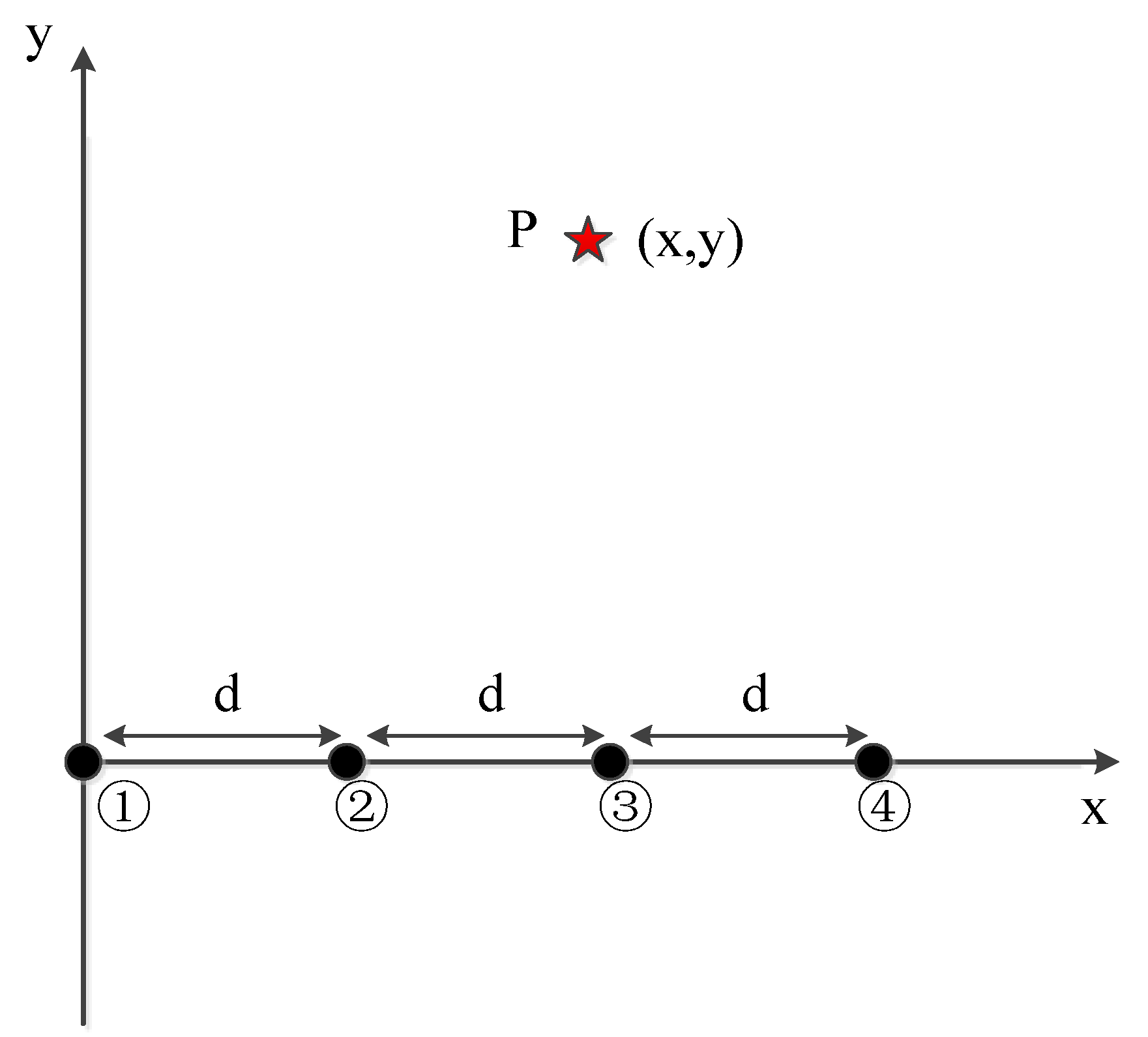
2.1. TDOA Method for Four Sensors

Four sensors linear arrays are used for locating here. The sensor arrangement is shown in Figure 1. Four sensors (①, ②, ③, and ④ in Figure 1) arranged adjacent to each other at equal intervals and P is the location of AE source. Suppose the distance between two adjacent sensors is d and the speed of AE wave is v. The time that AE signal generated by AE source P (x,y) reaches the sensor ① is t₁. The time differences of arrival between signal arrival times at sensor ②, ③, ④, and sensor ① are ∆t₂, ∆t₃, and ∆t₄, respectively. AE source coordinates satisfy the following relationships

$$\{\begin{array}{l}{x}^2+y^2=v^2{t}_1^2\\ {(x-d)}^2+y^2=v^2{(\Delta t_2+t_1)}^2\\ {(x-2d)}^2+y^2=v^2{(\Delta t_3+t_1)}^2\\ {(x-3d)}^2+y^2=v^2{(\Delta t_4+t_1)}^2\end{array}$$

(1)

By subtracting formula 1 from formula 2, 3, and 4 in Equation (1), we can get that

$$\{\begin{array}{l}-2xd+d^2=v^2(2t_1\Delta t_2+\Delta t_2^2)\\ -4xd+4d^2=v^2(2t_1\Delta t_3+\Delta t_3^2)\\ -6xd+9d^2=v^2(2t_1\Delta t_4+\Delta t_4^2)\end{array}$$

(2)

Then, we can get

$$t_1=\frac{3\Delta t_2{}^2-3\Delta t_3{}^2+\Delta t_4{}^2}{-6\Delta t_2+6\Delta t_3-2\Delta t_4}$$

(3)

Substituting Equation (3) into formula 1 and 2 in Equation (2), respectively, we can get unitary quadratic equations with x and v² as unknowns. Solving the equations, we can get

$$x=\frac{d\left(8t_1\Delta t_2+4\Delta t_2{}^2-2t_1\Delta t_3-\Delta t_3{}^2\right)}{8t_1\Delta t_2+4\Delta t_2{}^2-4t_1\Delta t_3-2\Delta t_3{}^2}$$

(4)

Dividing formula 1 by formula 2 in Equation (1), we can get

$$\frac{x^2+y^2}{{\left(x-d\right)}^2+y^2}=\frac{t_1{}^2}{{\left(\Delta t_2+t_1\right)}^2}$$

(5)

Solving Equation (5), we can get

$$y=\sqrt{\frac{t_1{}^2{d}^2-2xd{t}_1{}^2}{\Delta t_2{}^2+2\Delta t_2{t}_1}-x^2}$$

(6)

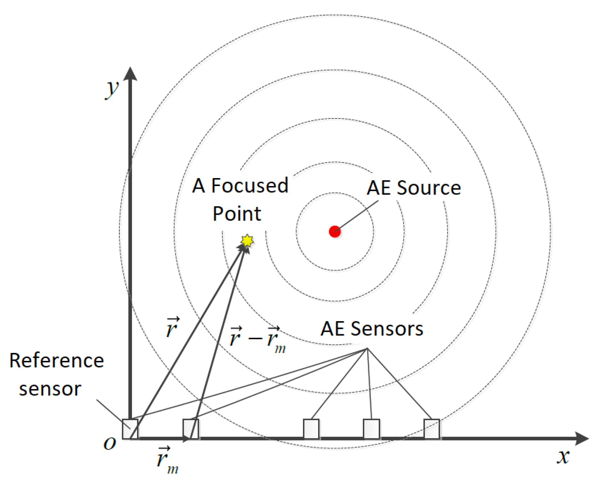
2.2. Beamforming Method

The beamforming method theoretically can identify the location of any AE source in the near-field region. When the array is focused to a point source at limited distance, the incident AE waves are spherical, as shown in Figure 2. Array output is calculated by [20]

$$b(\stackrel{\rightharpoonup }{r},t)=\frac{1}{M}{\displaystyle \sum _{m=1}^M{w}_m{x}_m(t-{\Delta }_m(\stackrel{\rightharpoonup }{r}))}$$

(7)

where $b(\stackrel{\rightharpoonup }{r},t)$ is the output of the array; $\stackrel{\rightharpoonup }{r}$ is the direction vector from the reference sensor to the focused point. The reference point may be arbitrary and it is the first sensor point on the left side in the Figure 2; M is the number of sensors; w_m the weighting coefficient for the channel of sensor m (usually no modification, in this article, $w_m\equiv 1$) and $x_m(t)$ represents the signal acquired from the No. m sensor; ${\Delta }_m(\stackrel{\rightharpoonup }{r})$ indicates the individual time delay of No. m sensor to the reference point.

By adjusting time delay ${\Delta }_m(\stackrel{\rightharpoonup }{r})$, the signals associated with the spherical waves, emitting from AE source focus, will be aligned in time before they are summed. As shown in Figure 2, ${\Delta }_m(\stackrel{\rightharpoonup }{r})$ can be obtained by

$${\Delta }_m(\stackrel{\rightharpoonup }{r})=\frac{\left|\stackrel{\rightharpoonup }{r}\right|-\left|\stackrel{\rightharpoonup }{r}-{\stackrel{\rightharpoonup }{r}}_m\right|}{c}$$

(8)

where ${\stackrel{\rightharpoonup }{r}}_m$ the distance between reference point and No. m sensor; $\left|\stackrel{\rightharpoonup }{r}\right|-\left|\stackrel{\rightharpoonup }{r}-{\stackrel{\rightharpoonup }{r}}_m\right|$ represents the difference between the distance from reference point to focus point and the distance from No. m sensor to the focus point; c is the propagation velocity of AE wave.

The output of the beamforming method is the integral of $b(\stackrel{\rightharpoonup }{r},t)$ over time, which has the meaning of energy. If the focused point is the real source, the signals are aligned at the same wave front and the output of the beamforming is maximum. However, the signals cannot be aligned at the same wave front when the array of sensors is focused on other locations, and the output of the beamforming is not the maximum. The location of the maximum output energy represents the location of the AE source. When the beamforming method is used, every point on the structure is focused, and the output of the beamforming array at every point needs to be calculated. Once the location of the real AE source is focused on, the output of the sensor array reaches the maximum value. Thus, the location of the real AE source can be judged by comparing those outputs. Figure 3 shows the operational principle of the beamforming method.

In operation, the localization accuracy can be determined according to actual needs. For example, on a 600 mm by 600 mm plate, if locating is performed with an accuracy of 10 mm, 3721 (61 × 61) points need to be scanned. If locating is performed with an accuracy of 1 mm, 361,201 (601 × 601) points need to be scanned. Obviously, the higher the localization accuracy, the more points need to be scanned. This means that the longer it takes to locate. Then the output of each point can be calculated. The point with the largest output value is the location of the acoustic emission source. Figure 4 shows the beamforming array output in a typical acoustic emission source location. At this time, normalization is performed according to the maximum output value. It can be seen from the Figure 4 that the location where the output is one is the acoustic emission source.

The beamforming method has high localization accuracy. However, the localization speed is very low since great quantities of points need to be scanned. The calculation speed is affected by the length of the calculation signal, the number of sensors, the localization accuracy (the higher the accuracy, the more points need to be scanned), and the size of the structure. Among these influencing factors, signal length, number of sensors, localization accuracy, and structural size are all rigid requirements, and it is difficult to change them for the speed of calculation.

3. Performance Analysis of TDOA Method and Beamforming Method Based on the Simulated Signals

Since the finite element simulation signal is close to the actual AE signal and easy to operate, this paper uses the simulation signal to study the performance of TDOA method and beamforming method for localizing AE source.

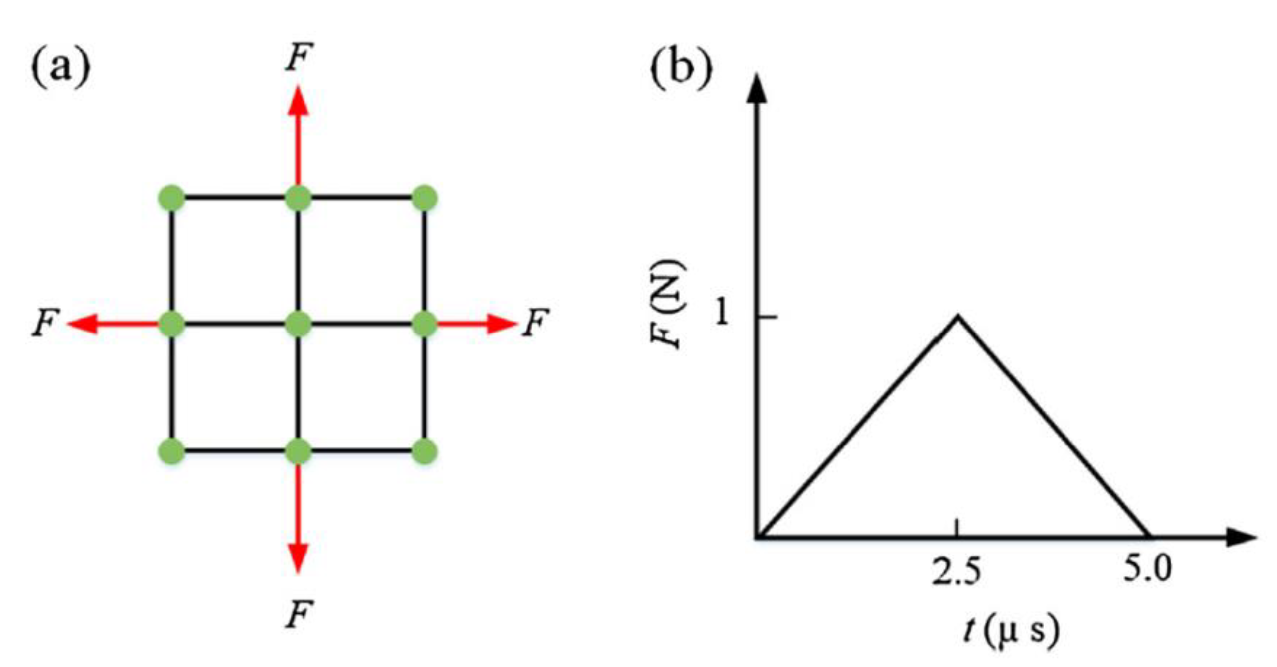
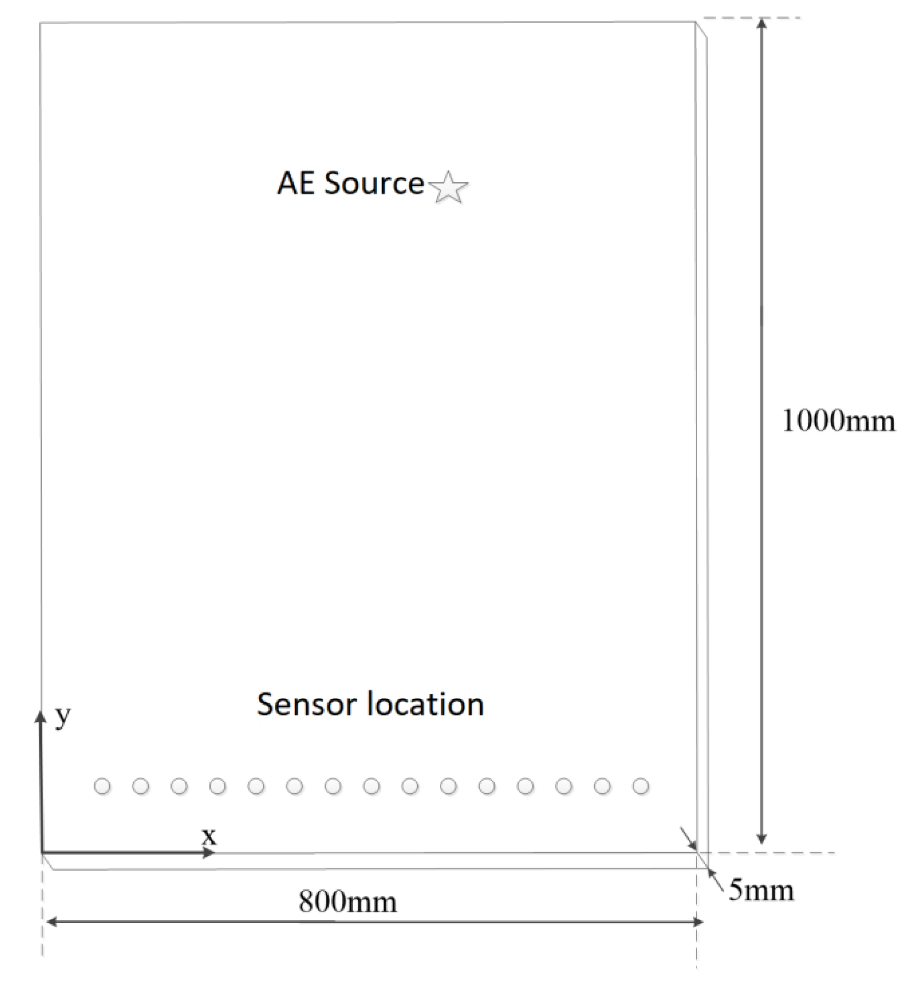
3.1. Simulation of AE Source

In this section, the commercial software Abaqus/Explicit is used to obtain the typical signals of the AE sources. In the simulation, the element type is C3D8R; the element size is 1 mm; the time increment step is set to be 1 × 10⁻⁸ s; the sampling interval is 2 × 10⁻⁷ s; and the total simulation time is 3 × 10⁻⁴ s. The quadrupole force is used to simulate AE source. As shown in Figure 5a, the concentrated forces with 1 N magnitude are loaded on the four nodes, respectively. The time history of these forces, as triangular pulse form, is shown in Figure 5b. Here, the S0 wave data are selected for localization.

3.2. Performance Analysis of TDOA Method

AE simulation is carried out on steel plates with dimensions of 800 mm by 1000 mm by 5 mm and the location of the 15 sensors is shown in Figure 6. The spacing of each sensor is 50 mm. The coordinates of the first sensor on the left are (50 mm, 100 mm). The location of AE source is set to #1 (300 mm, 600 mm) and #2 (500 mm, 800 mm). Material properties used in the finite element model are tabulated as

Table 1. Material properties.

Parameters	E	ρ	V
Value	209	7800	0.3
Units	GPa	Kg/m3	/

.

The simulated signals received by the 15 sensors are extracted for locating. Based on the first sensor on the left, the TDOA locating of four sensors is carried out according to the sensor spacing of 50 mm, 100 mm, 150 mm, and 200 mm, respectively. The localization results are shown in

Table 2. Time difference of arrival (TDOA) locating of different sensor spacing.

Sensor Spacing (mm)	Actual Location of #1 (mm)	Localization (mm)	Actual Location of #2 (mm)	Localization (mm)
50	(300, 600)	(286, 281)	(500, 800)	(650, 762)
100	(300, 600)	(300, 334)	(500, 800)	(534, 1010)
150	(300, 600)	(301, 381)	(500, 800)	(495, 757)
200	(300, 600)	(300, 586)	(500, 800)	(503, 834)

.

It can be concluded from Table 2 that the x-coordinates error located by the TDOA method of the four sensors for the linear array is small. When the x-coordinate of AE source is within the sensor array, the x-coordinate of the localization point is very accurate, but the y-coordinate is generally not accurate.

The relationship between the localization of four sensors and the TDOA error is studied by using the TDOA of ideal wave. Set AE wave propagation speed in the plate to 5400 m/s. AE source locations are selected as (350 mm, 600 mm), (550 mm, 600 mm), and (750 mm, 600 mm). Sensor spacing is 200 mm. The coordinates of number 1–4 sensors are (100 mm, 0 mm), (300 mm, 0 mm), (500 mm, 0 mm), and (700 mm, 0 mm). Firstly, it is assumed that the TDOA between the times of AE wave arriving at number 2 and 3 sensors to that of number 1 sensor remains unchanged. The TDOA between number 4 sensor and number 1 sensor is changed to deviate from within 10% of the correct value and observe the localization result. Then, it is assumed that the TDOA between the times of AE wave arriving at number 2 and 4 sensors to that of number 1 sensor remain unchanged. The TDOA between number 3 sensor and number 1 sensor is changed to deviate from within 10% of the correct value. Finally, it is assumed that the TDOA between the times of AE wave arriving at number 3 and 4 sensors to that of number 1 sensor are unchanged. The TDOA between the number 2 sensor and number 1 sensor is changed, and the deviation is also within 10% of the correct value. The localization results are shown in

Table 3. Localization results of changing TODA.

AE Source Location	Change in TODA (%)	Change ∆t2 Unchange ∆t3, ∆t4	Change ∆t3 Unchange ∆t2, ∆t4	Change ∆t4 Unchange ∆t2, ∆t3
(350, 600)	−10	N.A.	(345, 310)	(351, 383)
	−8	N.A.	(346, 340)	(351, 413)
	−6	N.A.	(347, 377)	(351, 447)
	−4	N.A.	(348, 426)	(350, 488)
	−2	(351, 1020)	(349, 495)	(350, 538)
	2	(349, 456)	(351, 801)	(350, 683)
	4	(348, 376)	(352, 1529)	(350, 800)
	6	(348, 323)	N.A.	(349, 992)
	8	(347, 284)	N.A.	(349, 1400)
	10	(347, 253)	N.A.	(349, 5150)
(550, 600)	−10	(560, 243)	N.A.	(525, 365)
	−8	(558, 280)	N.A.	(530, 396)
	−6	(556, 326)	N.A.	(534, 432)
	−4	(554, 386)	N.A.	(539, 476)
	−2	(552, 468)	(554, 1222)	(544, 530)
	2	(548, 880)	(547, 429)	(556, 696)
	4	(546, 4811)	(544, 338)	(563, 840)
	6	N.A.	(542, 279)	(570, 1096)
	8	N.A.	(540, 236)	(578, 1801)
	10	N.A.	(538, 202)	N.A.
(750, 600)	−10	(660, 112)	N.A.	(638, 299)
	−8	(675, 168)	N.A.	(653, 330)
	−6	(691, 233)	N.A.	(670, 369)
	−4	(709, 315)	N.A.	(691, 421)
	−2	(728, 427)	(835, 1702)	(717, 492)
	2	(774, 940)	(702, 372)	(795, 784)
	4	(802, 2844)	(672, 262)	(861, 1195)
	6	N.A.	(651, 195)	(965, 4644)
	8	N.A.	(637, 146)	N.A.
	10	N.A.	(626, 108)	N.A.

. N.A. indicates that the localization result has an imaginary number.

It can be concluded from Table 3 that when the TDOA fluctuates within a certain range, the localization result of the x-coordinate does not change much, but the range of the y-coordinate of the localization varies greatly. Sometimes the localization result may be an imaginary number.

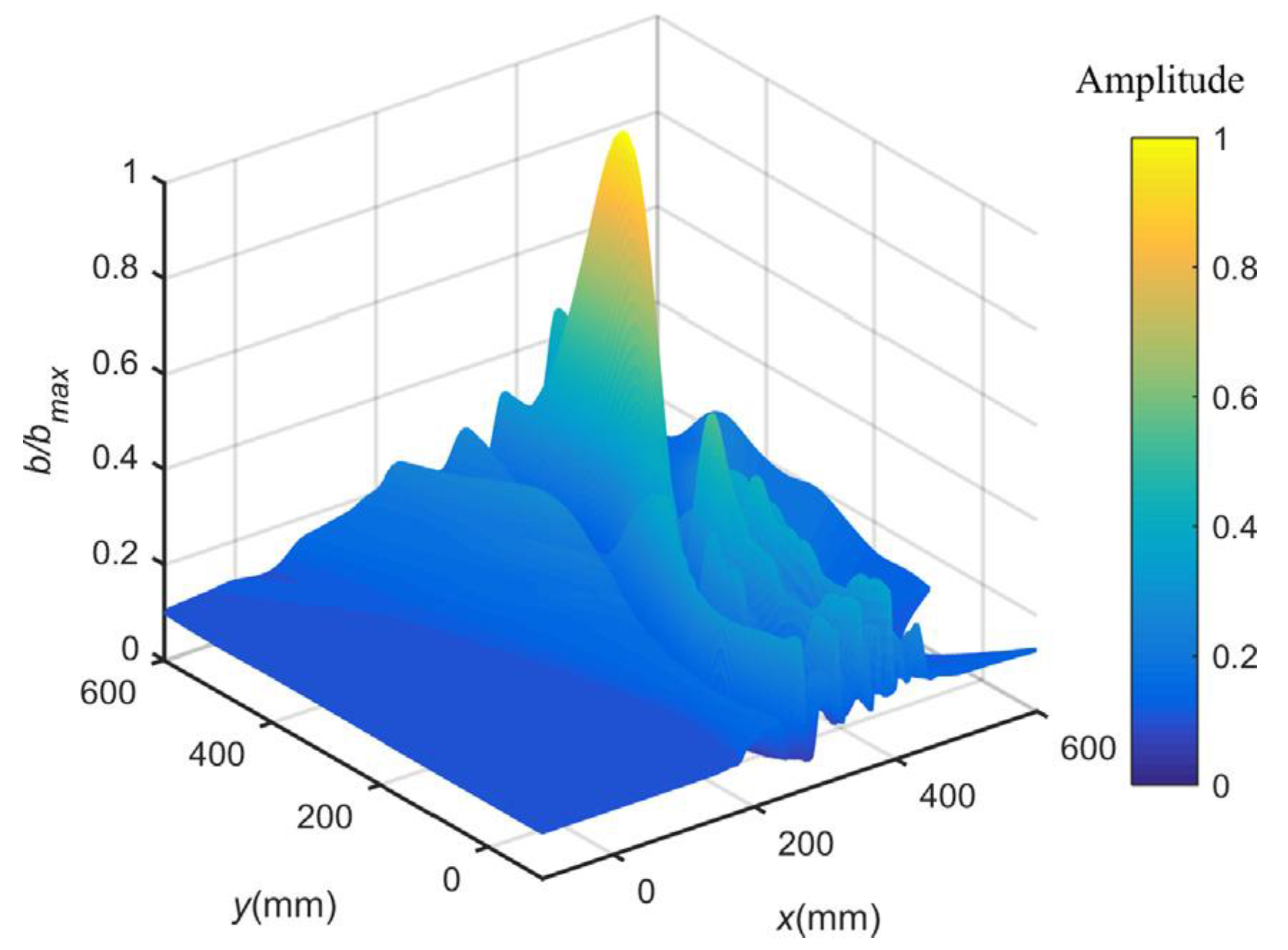
3.3. Performance Analysis of Beamforming Method

The simulation signals received by the above 15 sensors are extracted. The accuracy of 10 mm is used for beamforming method (same below). The number of points to be scanned is 8181 (101 × 81), and the beamforming locating is performed, respectively, according to the sensor spacings of 50 mm, 100 mm, 150, mm and 200 mm. According to the method and operation steps introduced in Section 2.2, the localization results are shown in

Table 4. Beamforming localization results.

Sensor Spacing (mm)	Actual Location of #1 (mm)	Localization (mm)	Actual Location of #2 (mm)	Localization (mm)
50	(300, 600)	(330, 690)	(500, 800)	(560, 940)
100	(300, 600)	(300, 610)	(500, 800)	(490, 800)
150	(300, 600)	(300, 610)	(500, 800)	(500, 820)
200	(300, 600)	(300, 610)	(500, 800)	(500, 820)

.

It can be seen from the localization results in Table 3 that the localization of the beamforming method is very accurate. As the distance between the sensors increases, the localization is more accurate. However, this method needs to divide the plate, and each divided point must be scanned and calculated, which increases the calculation cost.

4. Joint Localization Method for TDOA and Beamforming

From the above analysis, it can be known that if the four sensors are used for TDOA locating, the approximate location of AE source can be located. Then, the region located by the TDOA method is divided elaborately, and the beamforming method is used to locate AE source. This joint localization method is more accurate than the TDOA method, and also reduces the calculation cost in comparison to the beamforming method.

The specific steps are:

(1)

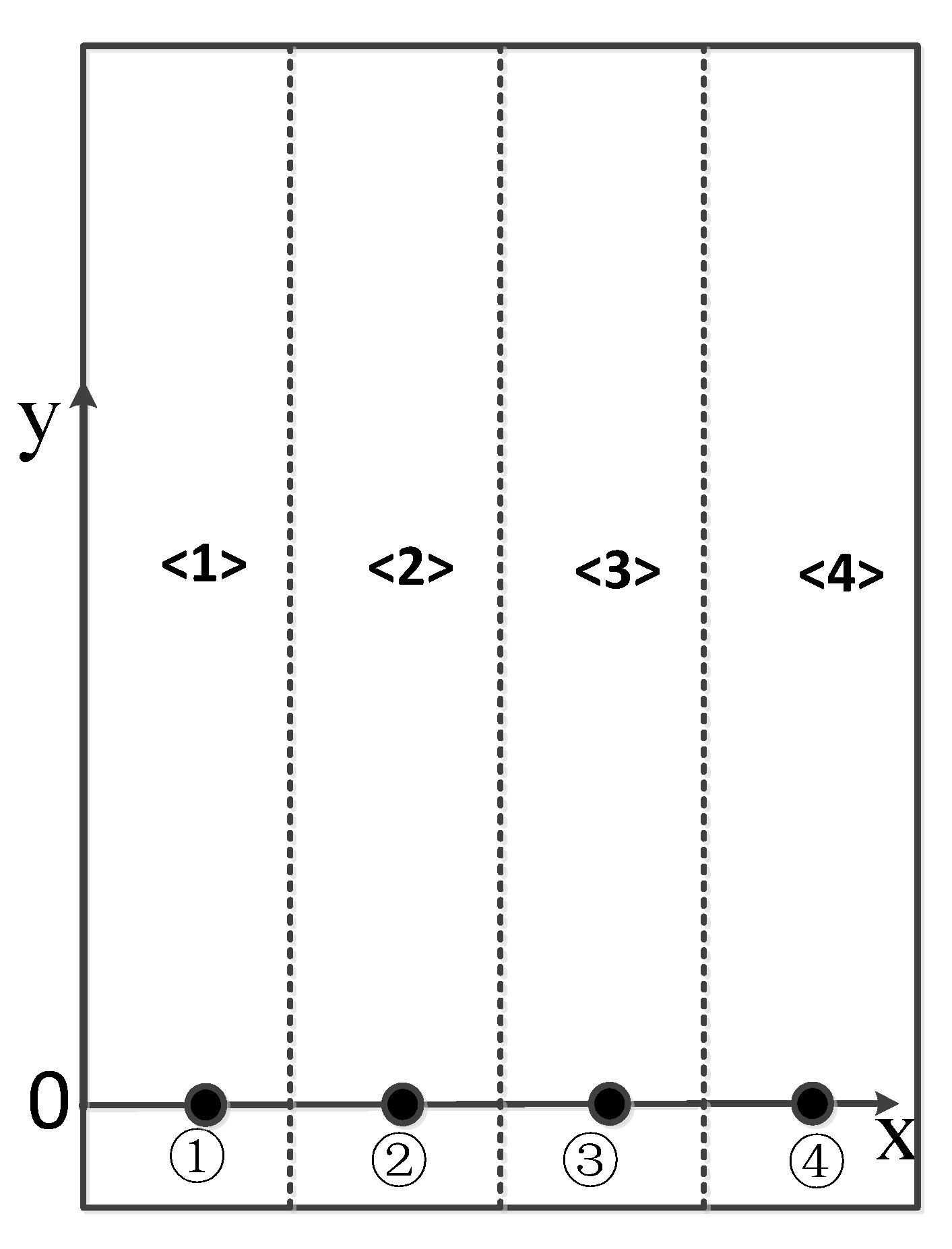
As shown in Figure 7, four sensors are placed on the plate which is divided according to the midpoint of each two adjacent sensors. Then the plate can be divided into four regions: <1>, <2>, <3>, and <4>. The sensors ➀–➃ are used for TDOA locating. The x-coordinate of the AE source can be obtained.

(2)

The localization based on the beamforming method is performed on the corresponding region according to the x coordinate. For example, if the x-coordinate of the TDOA locating is in the region <1>, the region <1> is subjected to the beamforming elaborate scanning for locating.

5. Simulation and Experimental Verification

In order to verify the effectiveness of the joint localization method proposed in this paper, the simulation is used to extract the signal for localization, and then the broken-lead experiment is performed on the steel plate.

5.1. Simulation Verification

AE simulation is carried out on steel plates with dimension of 800 mm by 700 mm by 5 mm. The sensors are arranged as Figure 5 with a spacing of 200 mm. The x-coordinates of AE source are set to 350 mm, 450 mm, 550 mm, 550 mm, and 750 mm, respectively, and the y-coordinates are set to 300 mm, 400 mm, 500 mm, and 600 mm, respectively. According to the method and operation steps introduced in Section 2.2, the localization results are shown in

Table 5. Simulation localization results.

Actual Location		TDOA Localization Result (mm)	Beamforming Scanning Region	Beamforming Localization Result (mm)
x (mm)	y (mm)
350	600	(350, 614)	<2>	(350, 610)
450		(450, 614)	<3>	(450, 610)
550		(550, 608)	<3>	(550, 610)
650		(549, 579)	<4>	(650, 620)
750		(647, 571)	<4>	(750, 630)
350	500	(350, 486)	<2>	(350, 510)
450		(450, 486)	<3>	(450, 510)
550		(550, 508)	<3>	(550, 510)
650		(650, 522)	<4>	(650, 520)
750		(746, 470)	<4>	(750, 530)
350	400	(350, 410)	<2>	(350, 410)
450		(450, 410)	<3>	(450, 410)
550		(550, 404)	<3>	(550, 410)
650		(649, 390)	<4>	(650, 420)
750		(748, 393)	<4>	(760, 440)
350	300	(350, 284)	<2>	(350, 310)
450		(450, 284)	<3>	(450, 310)
550		(550, 292)	<3>	(550, 310)
650		(650, 305)	<4>	(650, 320)
750		(750, 294)	<4>	(750, 330)

.

From Table 5, it can be concluded that after the x-coordinates of AE source are initially located by the TDOA method, the beamforming localization is carried out, and the localization results are more accurate. Due to the beamforming method scanning a quarter of the entire plate, the calculation cost of the localization is greatly reduced. The TDOA localization results in the Table 5 are also relatively accurate because the signal from the simulation data has no noise interference. There is a certain error in the actual TDOA.

5.2. Experimental Verification

In order to further verify the feasibility of joint localization method proposed in this paper, the broken-lead experiment is performed on the steel plate, as shown in Figure 8. It includes four AE sensors connected to the preamplifier to obtain the signal, and the data acquisition instrument connected to the PC to analyze and process the signal. The sensors are arranged in a row with coordinates (150 mm, 0 mm), (270 mm, 0 mm), (390 mm, 0 mm), and (510 mm, 0 mm), respectively. The sensor spacing is 120 mm. The broken-lead experiments are performed at the location of AE sources shown in

Table 6. Experimental localization results.

Actual Location		TDOA Localization Result (mm)	Beamforming Scanning Region	Beamforming Localization Result (mm)
x (mm)	y (mm)
100	600	(−42, N.A.)	<1>	(100, 560)
160	600	(113, N.A.)		(160, 590)
220	210	(215, 71)	<2>	(220, 200)
	450	(220, N.A.)		(220, 440)
	510	(196, N.A.)		(220, 500)
280	270	(280, 394)		(280, 260)
	390	(283, 598)		(280, 390)
340	330	(343, N.A.)	<3>	(340, 330)
	500	(344, N.A.)		(340, 500)
400	270	(402, 224)		(400, 250)
	390	(403, 253)		(410, 400)
560	210	(460, 169)	<4>	(560, 190)
	450	(467, 229)		(570, 450)
	510	(454, 212)		(570, 530)

, and the signal received by the sensors are extracted. According to the method and operation steps introduced in Section 2.2, the localization results are shown in Table 6. N.A. indicates that the localization result has an imaginary number.

It can be seen from Table 6 that when the experimental data are used for TDOA localization, the x-coordinates location are accurate, but the y-coordinates error are relatively large. However, the beamforming localization results are very accurate.

Table 7. The comparison of the average calculation time between the beamforming method and the joint localization method under different localization accuracy.

Localization Accuracy (mm)	Beamforming Method (s)	Joint Localization Method (s)
10	2.03	0.53
5	8.49	2.46
2	49.16	12.08
1	193.26	50.67
0.5	780.19	198.16
0.2	4887.19	1234.80

shows the comparison of the average calculation time between the beamforming method and the joint localization method proposed in this paper under different localization accuracy. Since beamforming scans only a quarter of the steel plate, the localization time of joint localization method is about a quarter of that of beamforming method. For large structures or high-precision localization, the benefits of using the joint localization method are obvious. At the same time, the memory requirements of the computer are reduced.

6. Conclusions

This paper proposes a novel joint localization method of AE source based on TDOA method and beamforming method. By using the AE signal from finite element simulation, the performance of TDOA method and beamforming method of four sensors arranged on the plate are studied in detail. Aiming at the advantages and disadvantages of the performance of the two methods, a joint localization method is proposed. The performance of joint localization method is verified by simulation and experiment. Both simulation and experimental results show that the joint localization method not only improves the accuracy of the TDOA method, but also greatly reduces the localization calculation cost of the beamforming method.

References

1. Wells, R.; Hamstad, M.A.; Mukherjee, A.K. On the origin of the first peak of acoustic emission in 7075 aluminum alloy. J. Mater. Sci. 1983, 18, 1015–1020. [Google Scholar] [CrossRef]
2. Sause, M.G.R.; Horn, S. Simulation of lamb wave excitation for different elastic properties and acoustic emission source geometries. J. Acoust. Emiss. 2010, 28, 142–154. [Google Scholar]
3. Lin, L.; Chu, F. HHT-based AE characteristics of natural fatigue cracks in rotating shafts. Mech. Syst. Signal Process. 2012, 26, 181–189. [Google Scholar] [CrossRef]
4. Wang, Q.; Chu, F. Experimental determination of the rubbing location by means of acoustic emission and wavelet transform. J. Sound Vibr. 2001, 248, 91–103. [Google Scholar] [CrossRef]
5. Kundu, T.; Das, S.; Martin, S.A.; Jata, K.V. Locating point of impact in anisotropic fiber reinforced composite plates. Ultrasonics 2008, 48, 193–201. [Google Scholar] [CrossRef] [PubMed]
6. Kundu, T. Acoustic Source Localization. Ultrasonics 2014, 54, 25–38. [Google Scholar] [CrossRef] [PubMed]
7. Tobias, A. Acoustic-Emission Source Location in Two Dimensions by an Array of Three Sensors. Non-Destr. Test. 1976, 9, 9–12. [Google Scholar] [CrossRef]
8. Ahadi, M.; Bakhtiar, M.S. Leak Detection in Water-Filled Plastic Pipes through the Application of Tuned Wavelet Transforms to Acoustic Emission Signals. Appl. Acoust. 2010, 71, 634–639. [Google Scholar] [CrossRef]
9. McLaskey, G.C.; Glaser, S.D.; Grosse, C.U. Beamforming Array Techniques for Acoustic Emission Monitoring of Large Concrete Structures. J. Sound Vib. 2010, 329, 2384–2394. [Google Scholar] [CrossRef]
10. He, T.; Pan, Q.; Liu, Y.; Liu, X.; Hu, D. Near-field beamforming analysis for acoustic emission source localization. Ultrasonics 2012, 52, 587–592. [Google Scholar] [CrossRef] [PubMed]
11. Nakatani, H.; Hajzargarbashi, T.; Ito, K.; Kundu, T.; Takeda, N. Impact localization on a cylindrical plate by near-field beamforming analysis. In Sensors and Smart Structures Technologies for Civil, Mechanical, and Aerospace Systems 2012; International Society for Optical Engineering: San Diego, CA, USA, 2012; Volume 8345, p. 83450Y. [Google Scholar] [CrossRef]
12. Nakatani, H.; Hajzargarbashi, T.; Ito, K.; Kundu, T.; Takeda, N. Locating Point of Impact On An Anisotropic Cylindrical Surface Using Acoustic Beamforming Technique. Key Eng. Mater. 2013, 558, 331–340. [Google Scholar] [CrossRef]
13. Kundu, T.; Das, S.; Jata, K.V. Point of impact prediction in isotropic and anisotropic plates from the acoustic emission data. J. Acoust. Soc. Am. 2007, 122, 2057–2066. [Google Scholar] [CrossRef] [PubMed]
14. Kundu, T.; Das, S.; Jata, K.V. Detection of the Point of Impact on a Stiffened Plate by the Acoustic Emission Technique. Smart Mater. Struct. 2009, 18, 35006. [Google Scholar] [CrossRef]
15. Hajzargerbashi, T.; Kundu, T.; Bland, S. An Improved Algorithm for Detecting Point of Impact in Anisotropic Inhomogeneous Plates. Ultrasonics 2011, 51, 317–324. [Google Scholar] [CrossRef] [PubMed]
16. Koabaz, M.; Hajzargarbashi, T.; Kundu, T.; Deschamps, M. Locating the Acoustic Source in An Anisotropic Plate. Struct. Health Monit. 2011, 11, 315–323. [Google Scholar] [CrossRef]
17. Kundu, T. A New Technique for Acoustic Source Localization in an Anisotropic Plate without Knowing Its Material Properties. In Proceedings of the 6th European Workshop on Structural Health Monitoring, Dresden, Germany, 3–6 July 2012; pp. 37–45. [Google Scholar]
18. Kundu, T.; Nakatani, H.; Takeda, N. Acoustic Source Localization in Anisotropic Plates. Ultrasonics 2012, 52, 740–746. [Google Scholar] [CrossRef] [PubMed]
19. Nakatani, H.; Kundu, T.; Takeda, N. Improving accuracy of acoustic source localization in anisotropic plates. Ultrasonics 2014, 54, 1776–1788. [Google Scholar] [CrossRef] [PubMed]
20. He, T.; Xiao, D.; Pan, Q.; Liu, X. Analysis on accuracy improvement of rotor–stator rubbing localization based on acoustic emission beamforming method. Ultrasonics 2014, 54, 318–329. [Google Scholar] [CrossRef] [PubMed]
21. Liu, X.; Xiao, D.; Shan, Y.; Pan, Q.; He, T.; Gao, Y. Solder joint failure localization of welded joint based on acoustic emission beamforming. Ultrasonics 2017, 74, 221–232. [Google Scholar] [CrossRef] [PubMed]
22. He, T.; Tai, J.; Shan, Y.; Wang, X.; Liu, X. A Fast Acoustic Emission Beamforming Localization Method Based on Hilbert Curve. Mech. Syst. Signal Process. 2019, 133, 106291. [Google Scholar] [CrossRef]
Figure 1. Linear array of four sensors.
Applsci 10 08045 g001
Figure 2. Schematic diagram of the principle of beamforming method.
Applsci 10 08045 g002
Figure 3. The operational principle of the beamforming method.
Applsci 10 08045 g003
Figure 4. A typical energy output of beamforming method [22].
Applsci 10 08045 g004
Figure 5. Excitation information: (a) The loading location; (b) The mechanical representation.
Applsci 10 08045 g005
Figure 6. Steel plate simulation model.
Applsci 10 08045 g006
Figure 7. Schematic diagram of joint location method.
Applsci 10 08045 g007
Figure 8. Experimental setup of acoustic emission (AE) detection.
Applsci 10 08045 g008