Numerical Investigation on the Water Entry of Several Different Bow-Flared Sections


Abstract
1. Introduction
2. Mathematical Formulation and Numerical Methods
3. Computational Overview, Convergence, and Validation Studies
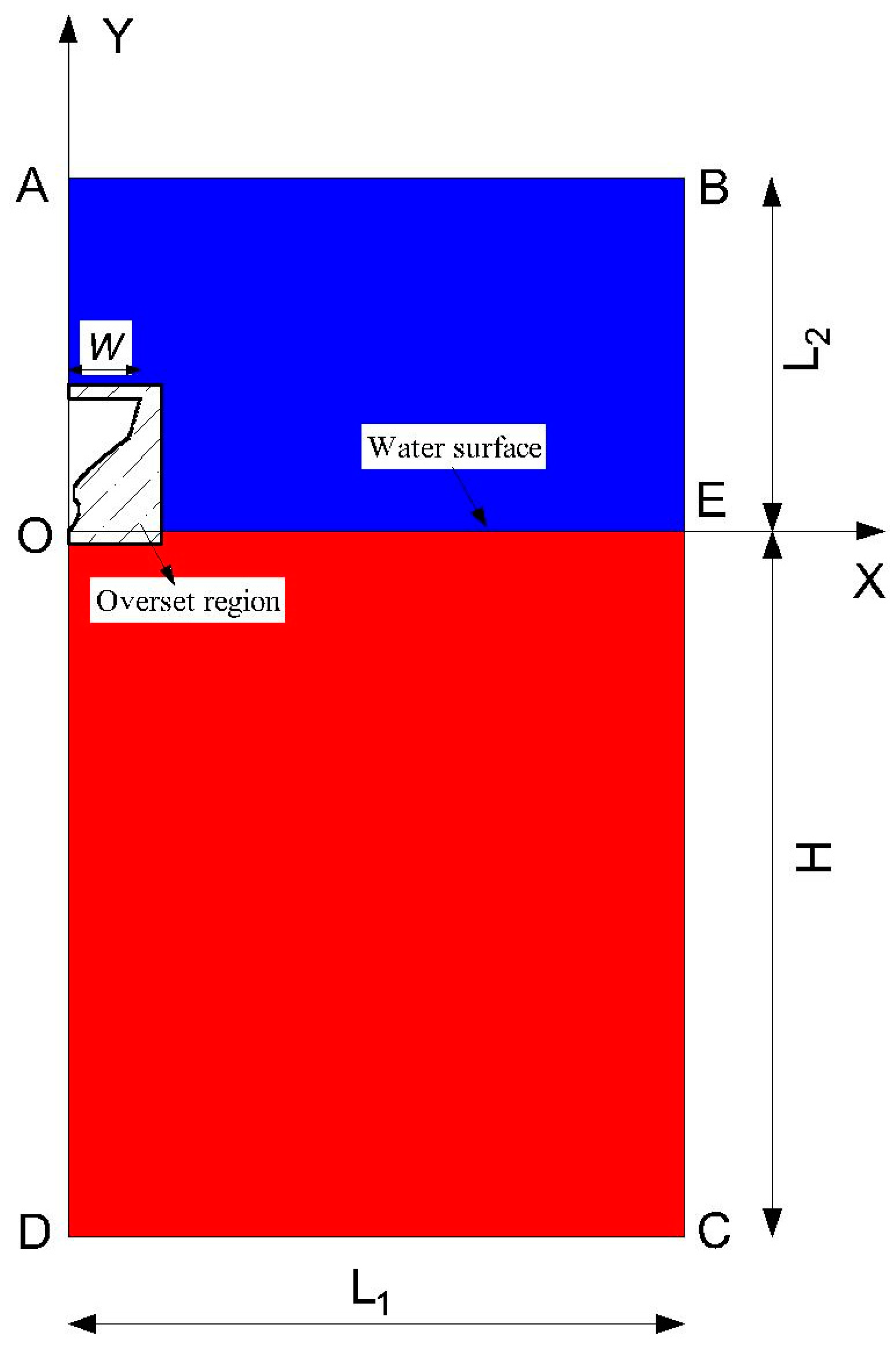
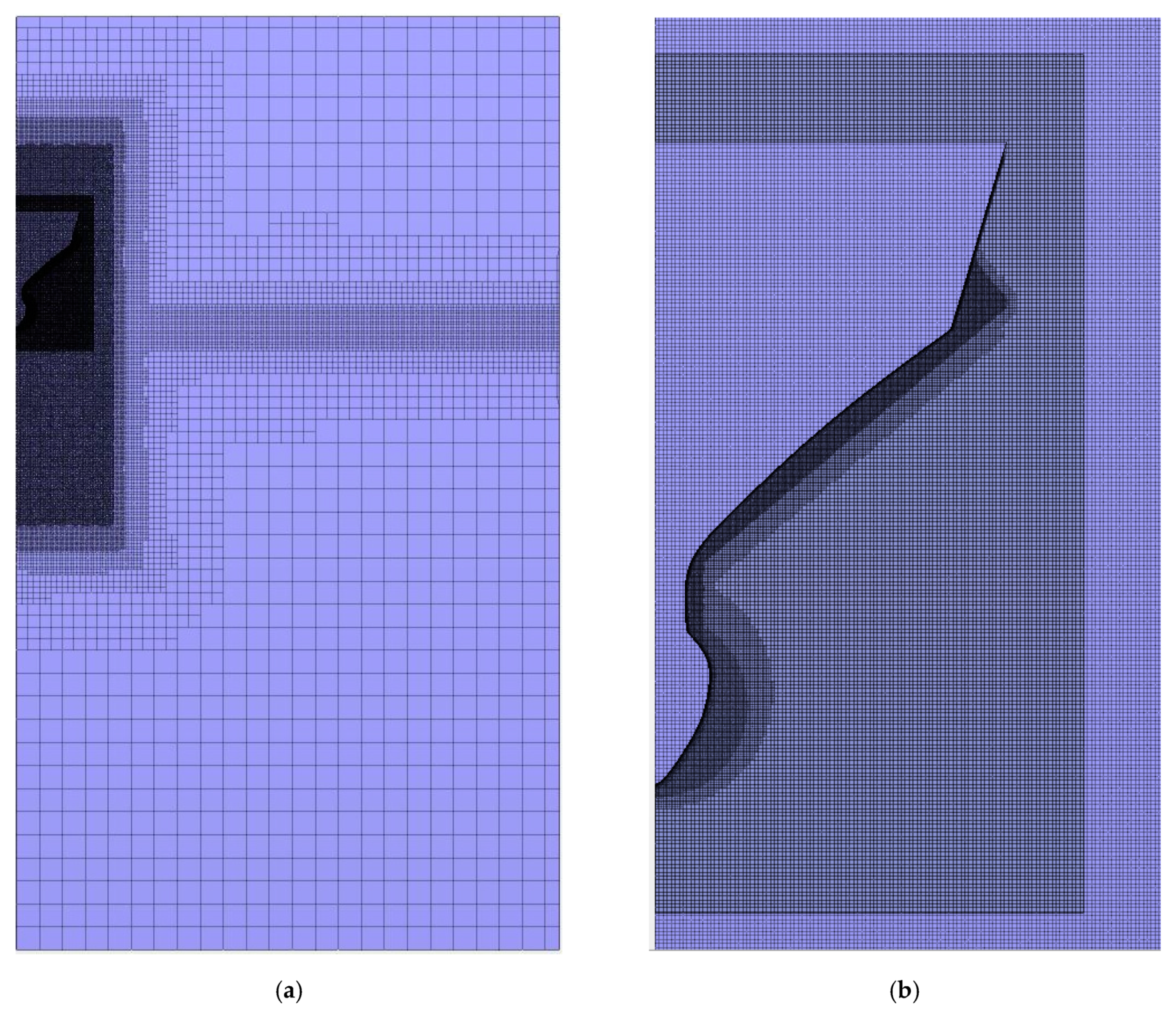
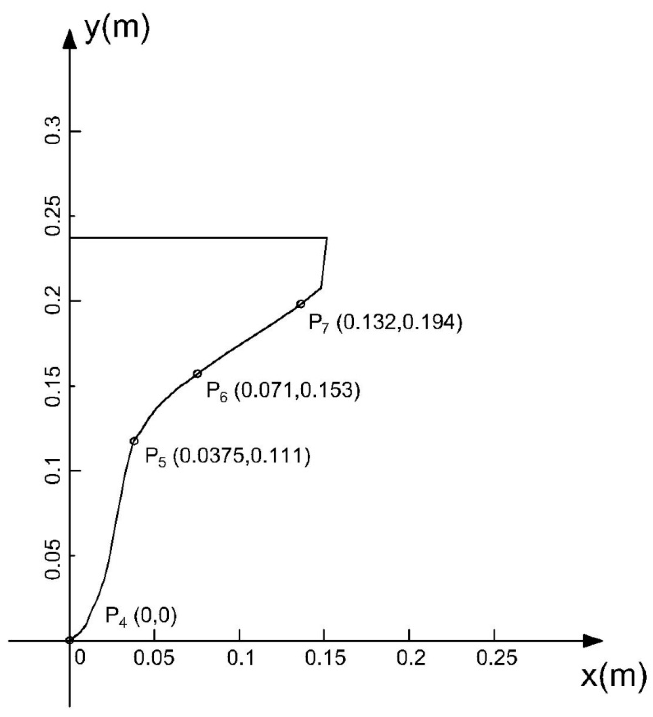
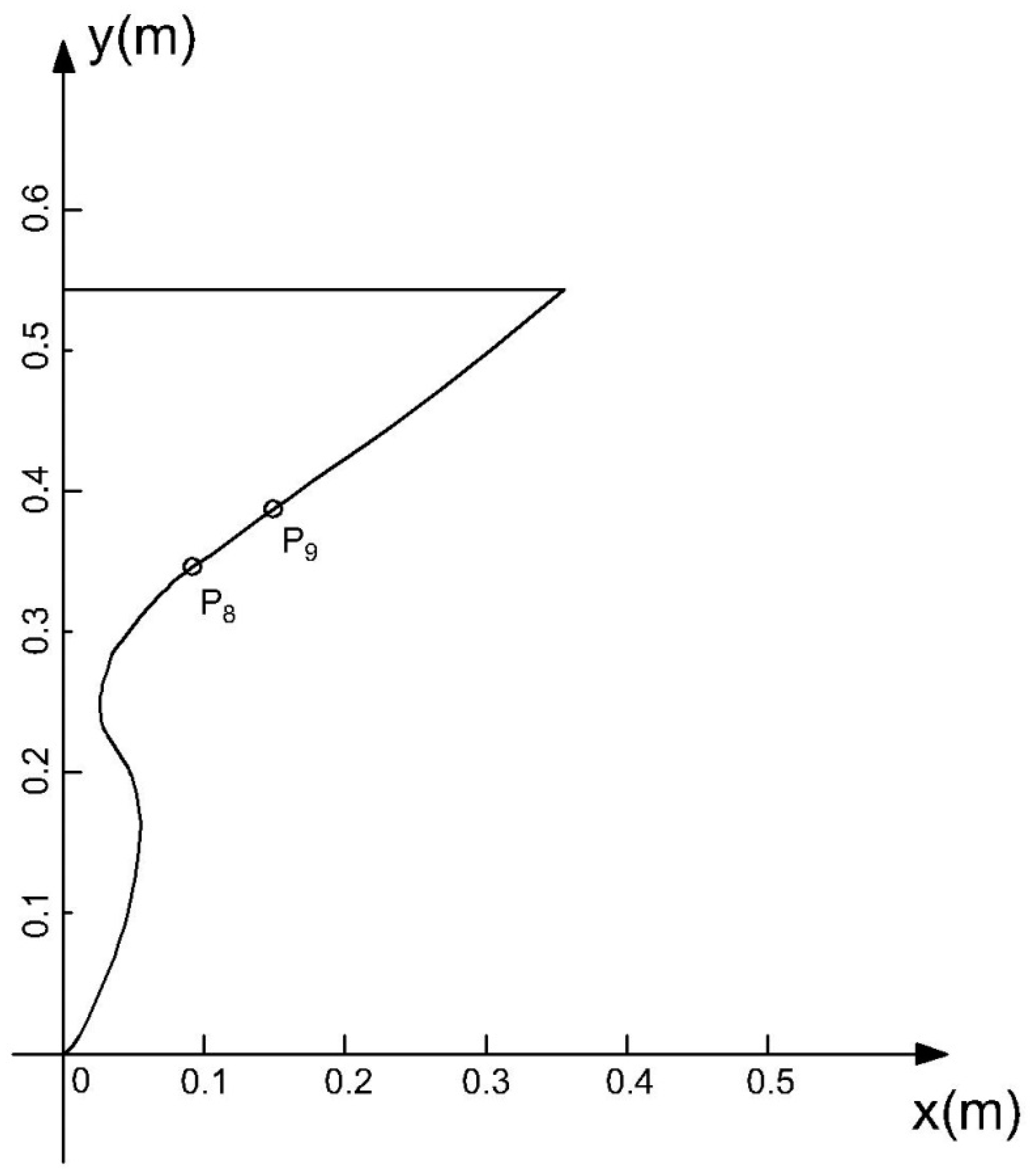
3.1. Computational Overview
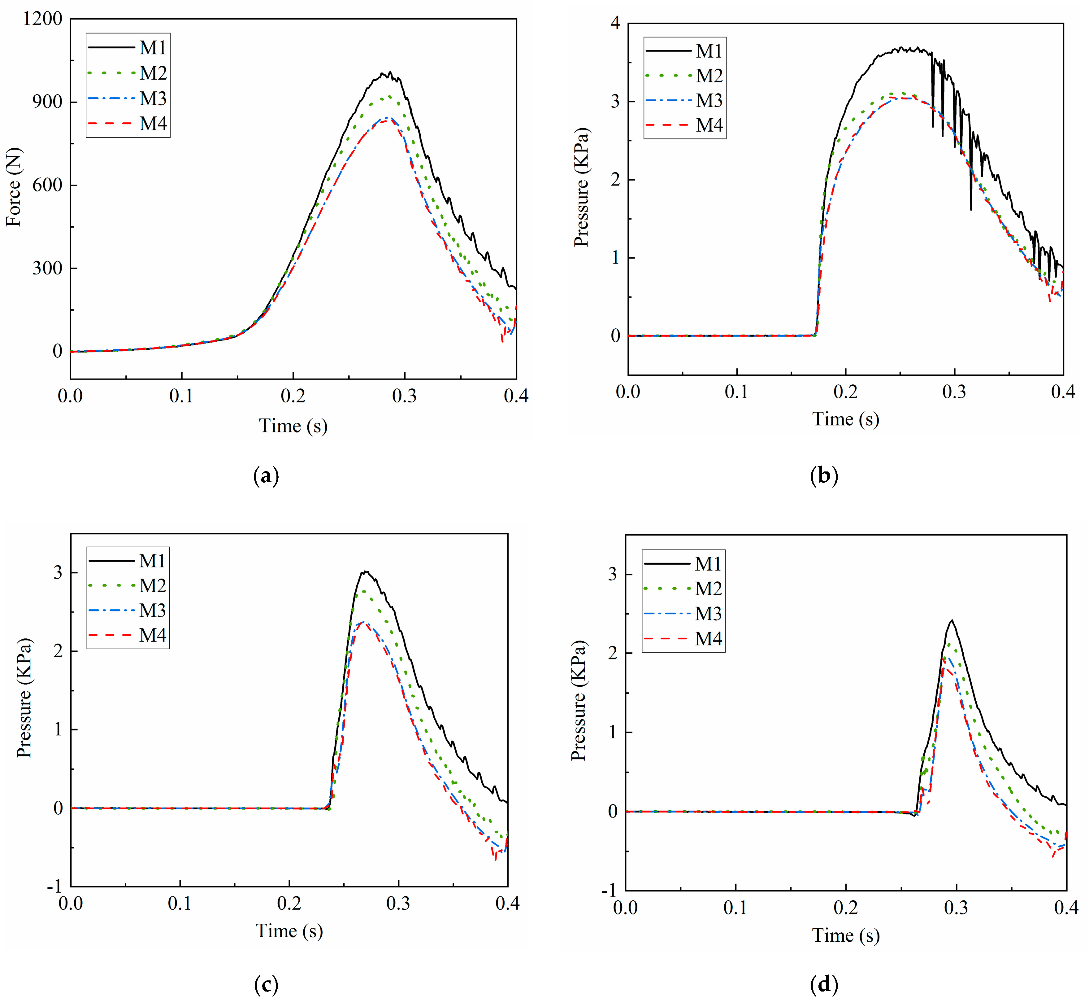
3.2. Convergence Study
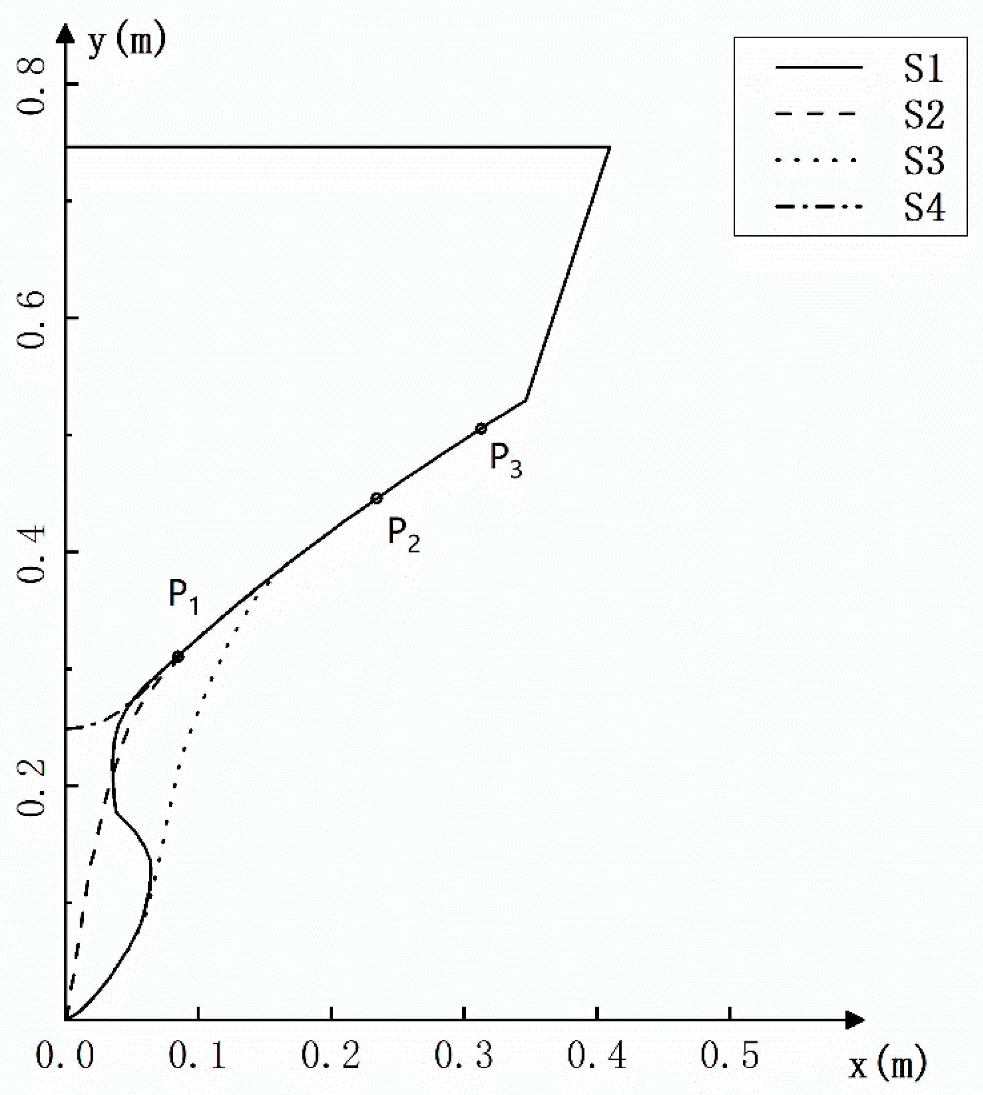
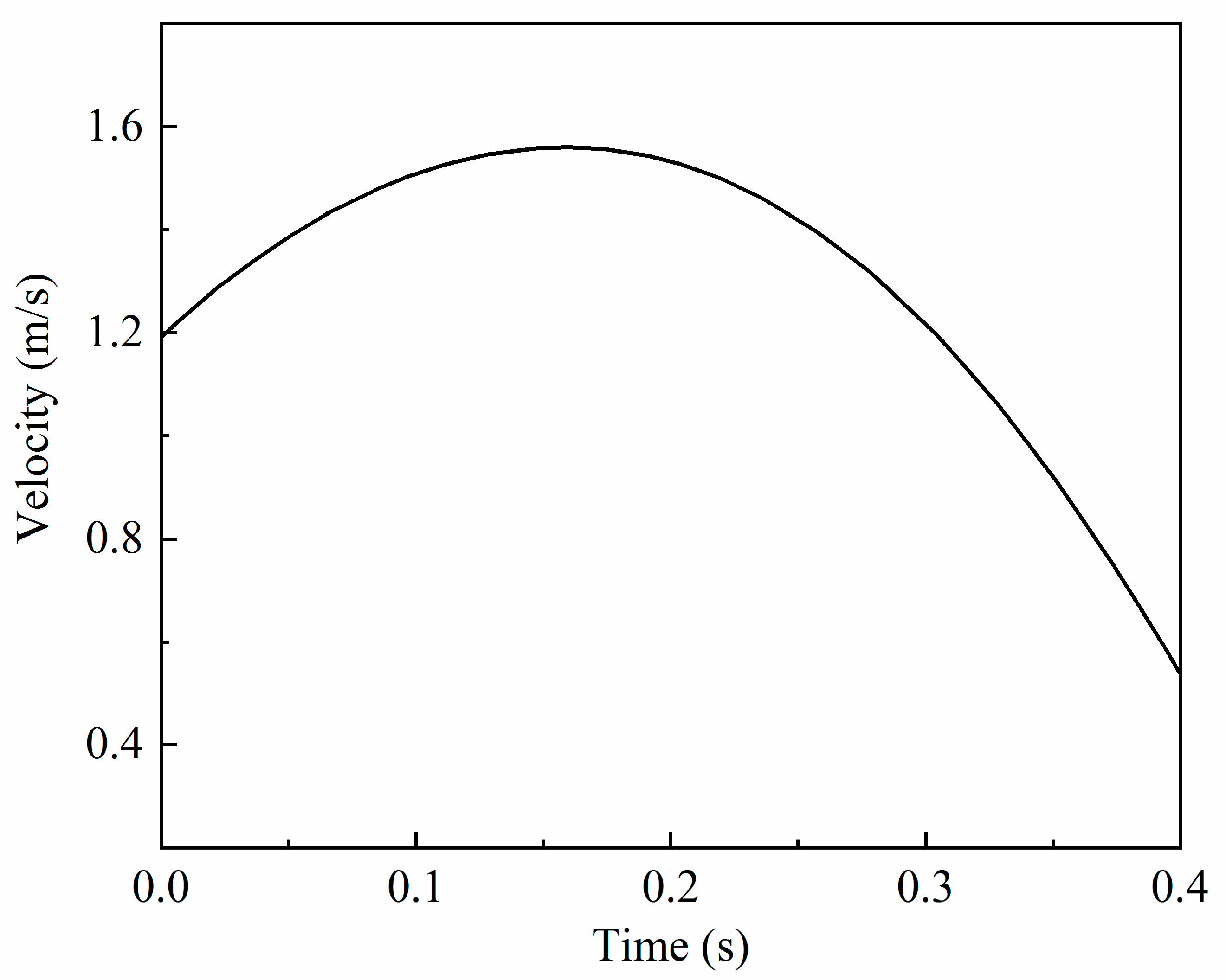
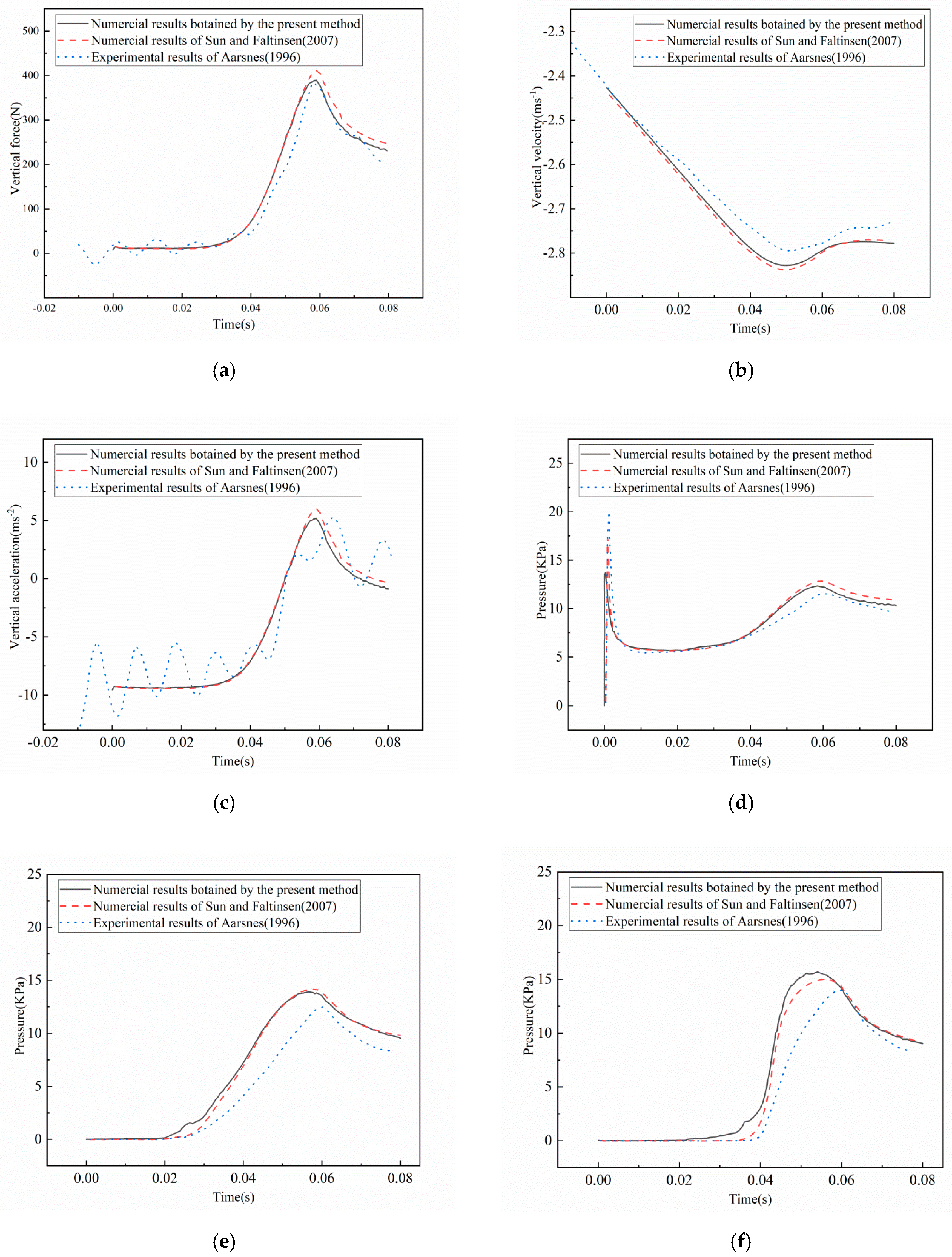
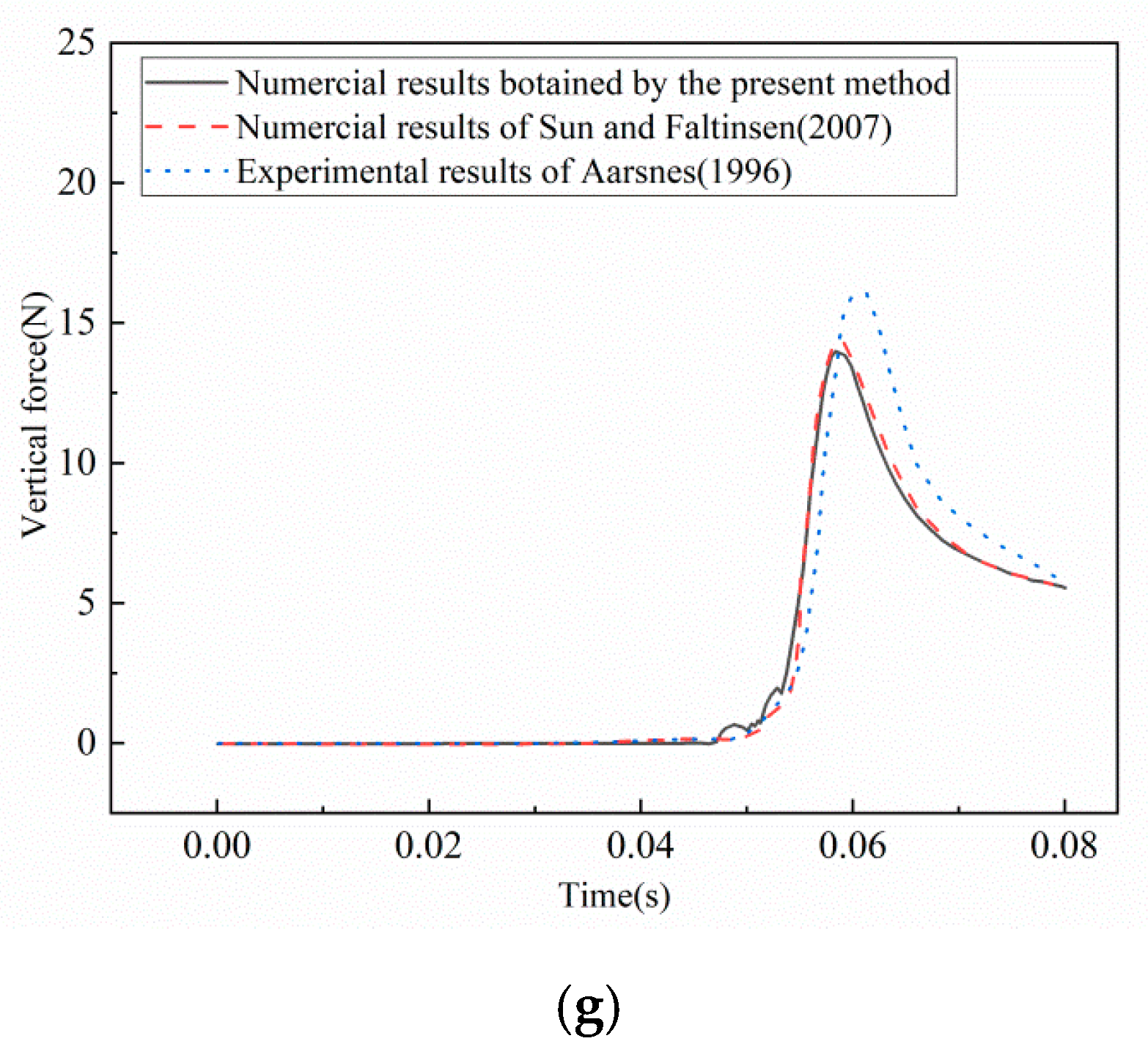
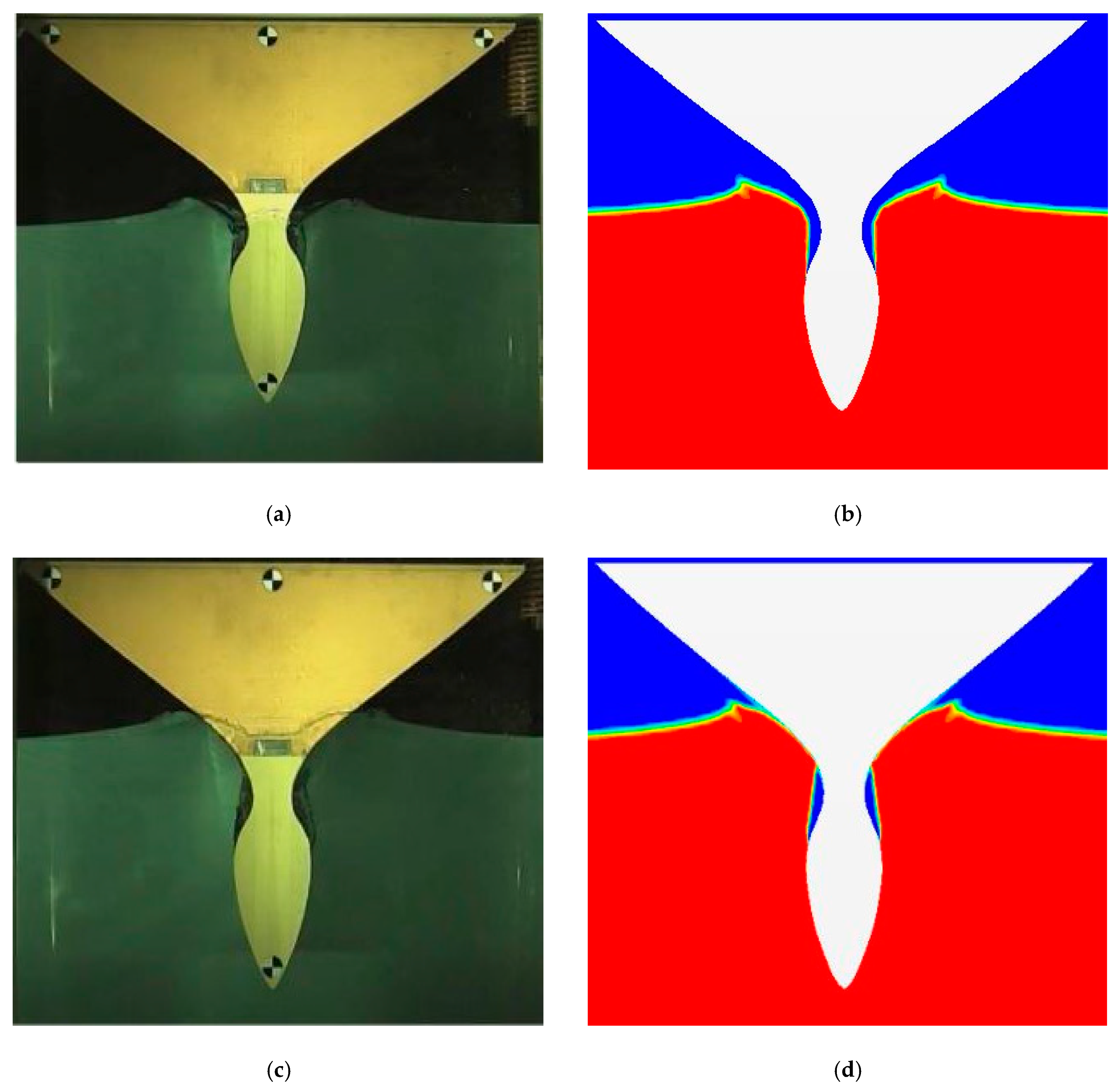
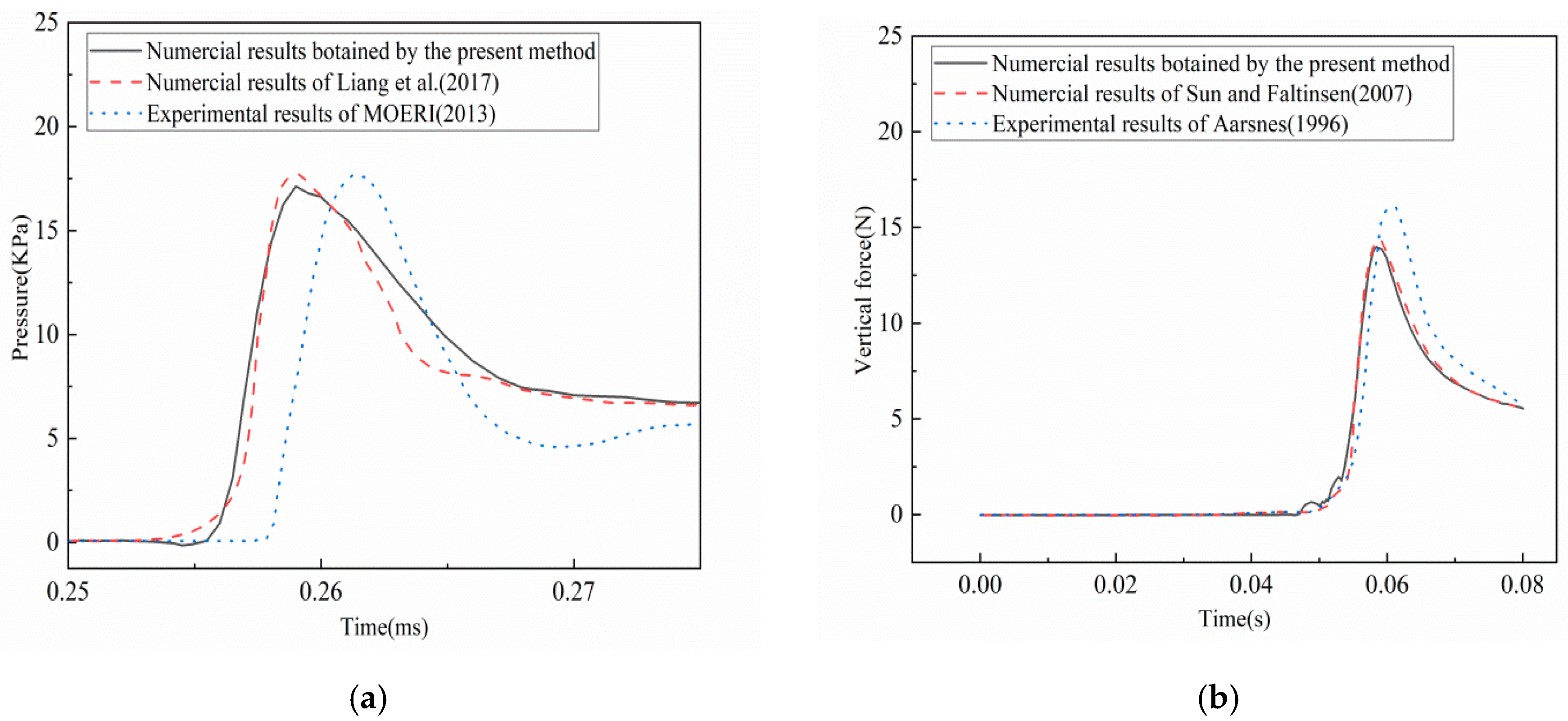
3.3. Validation Studies
4. Results and Discussions
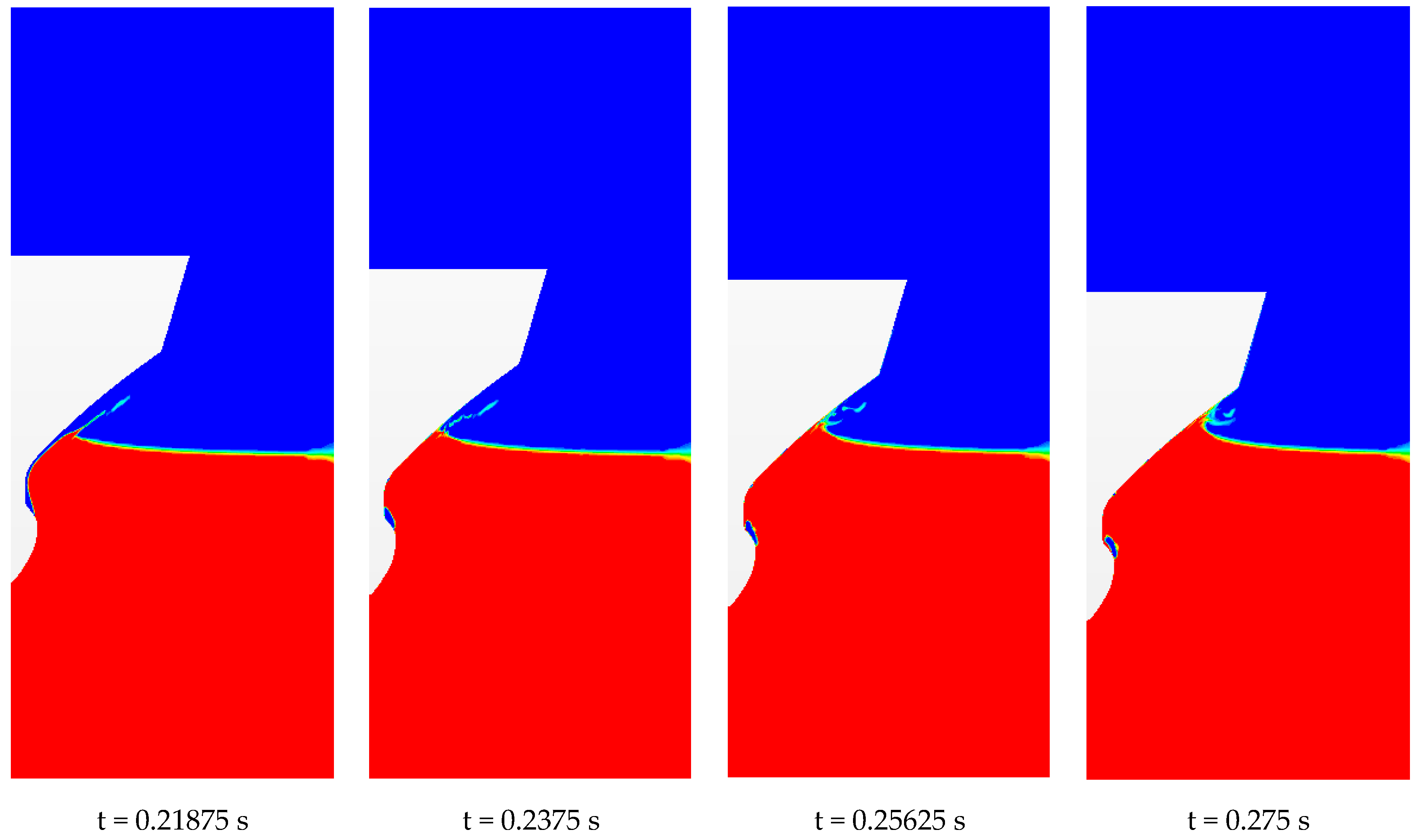
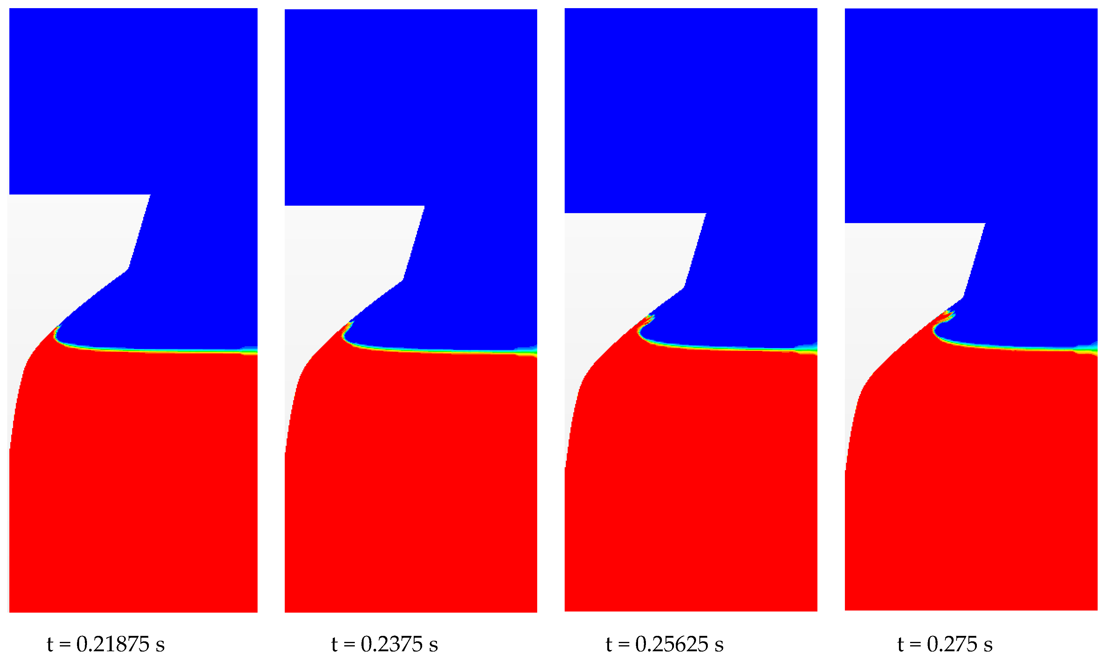
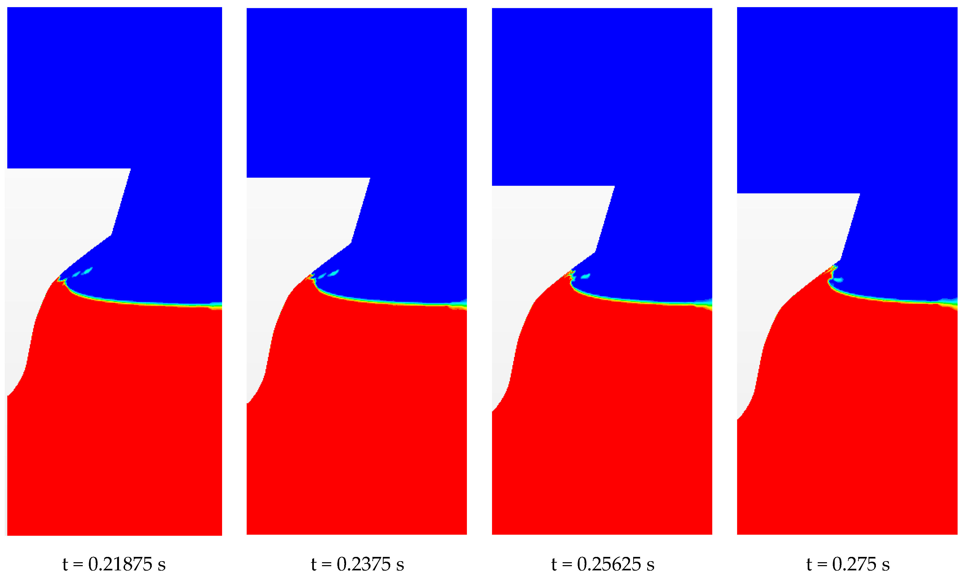
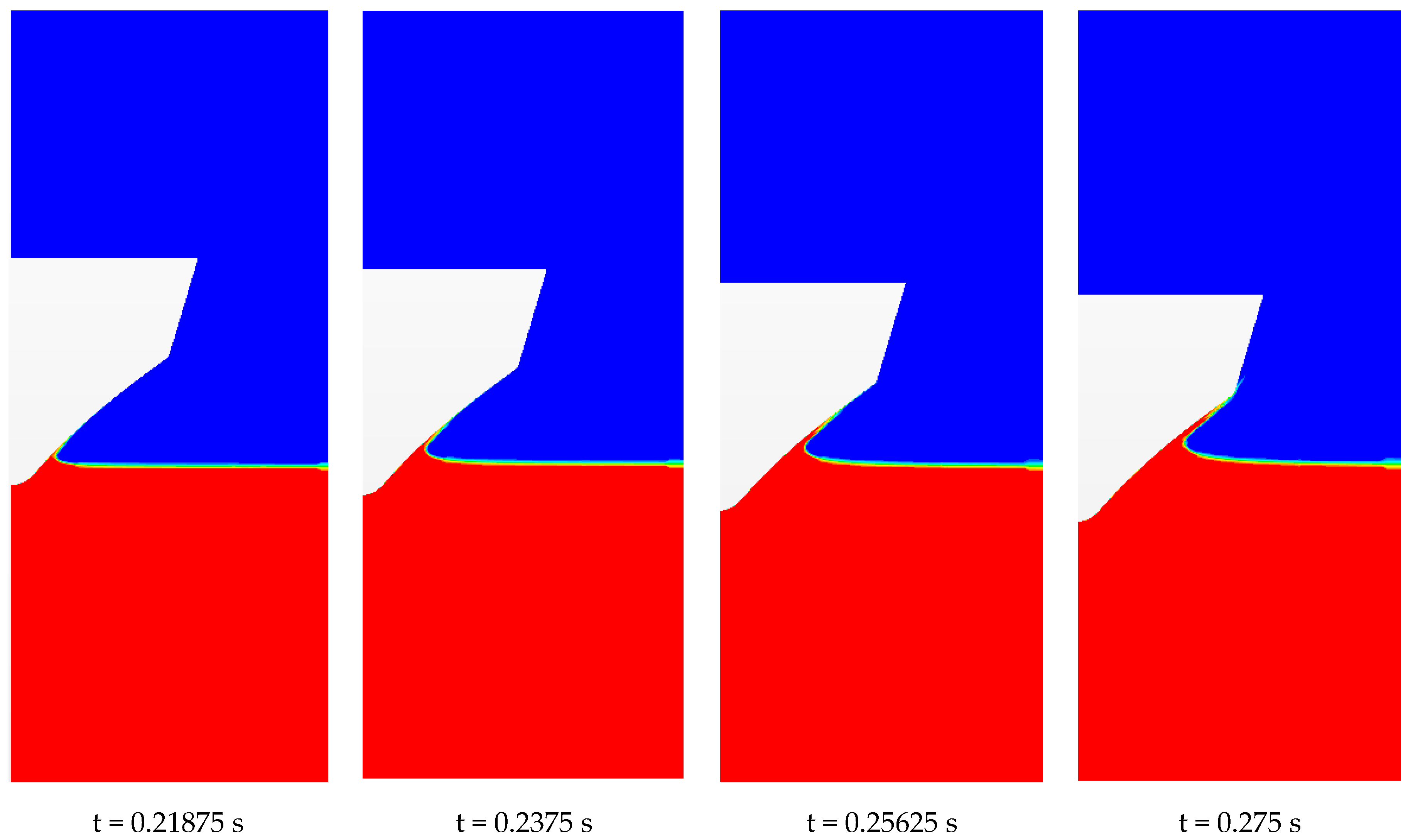
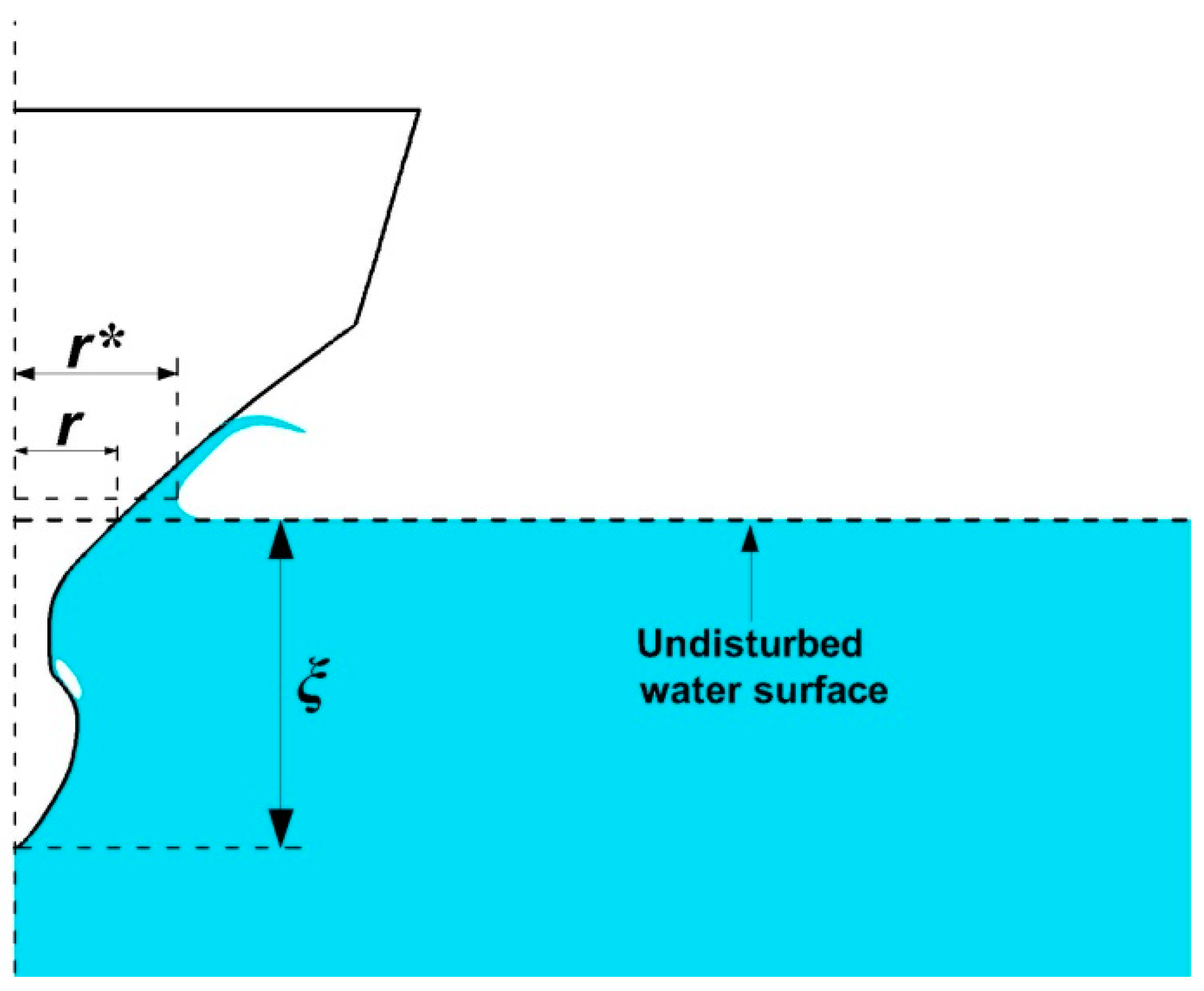
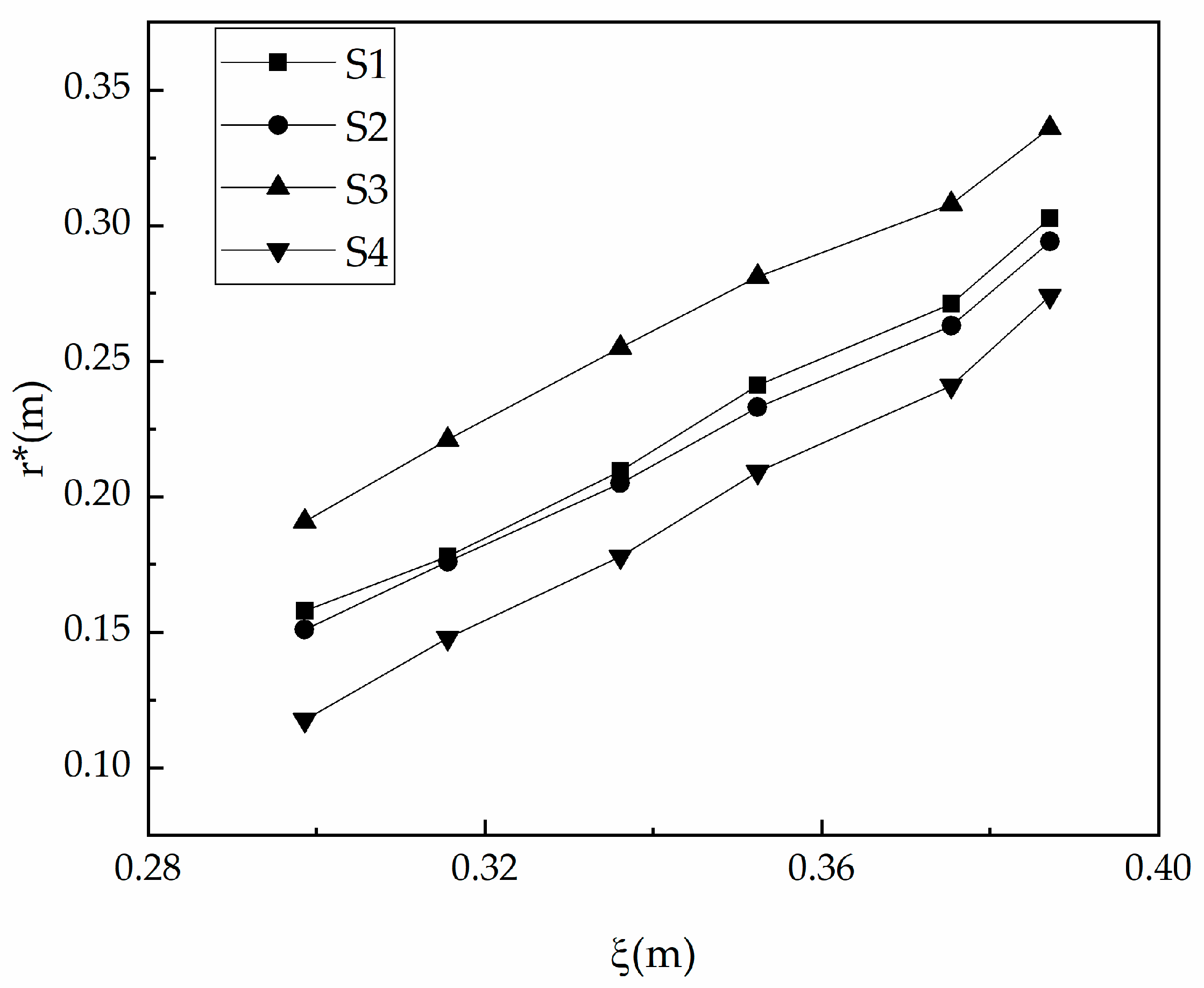
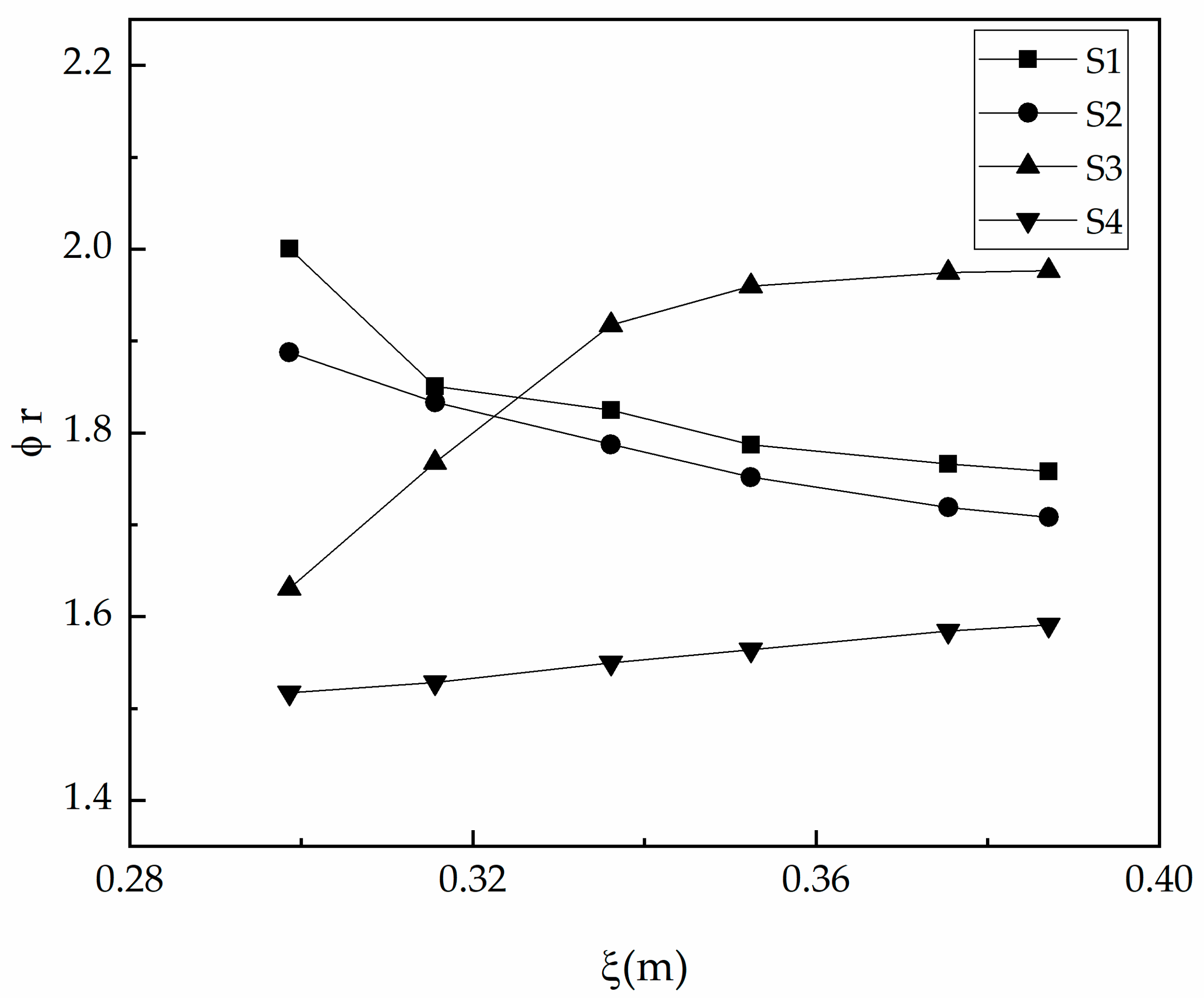
4.1. Free Surface Evolution
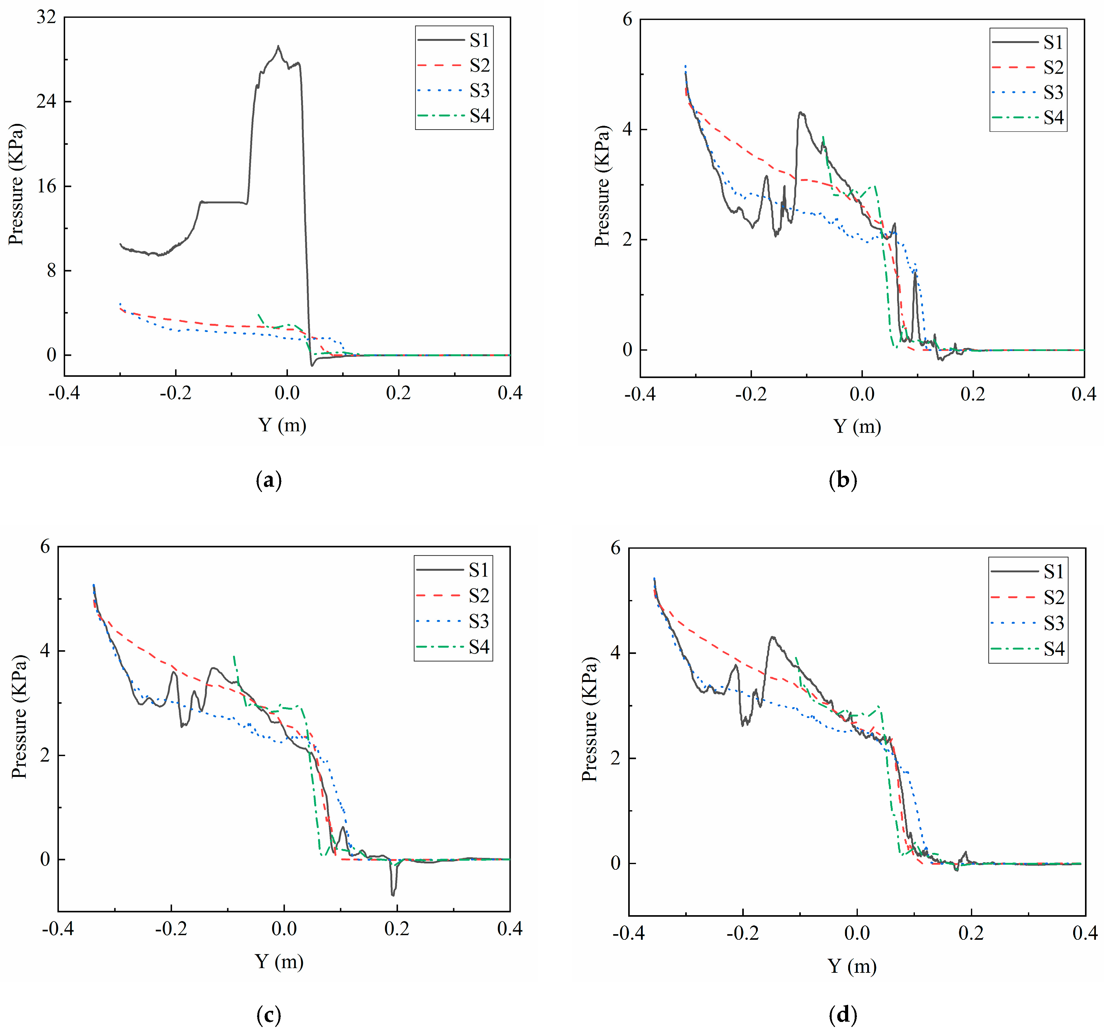
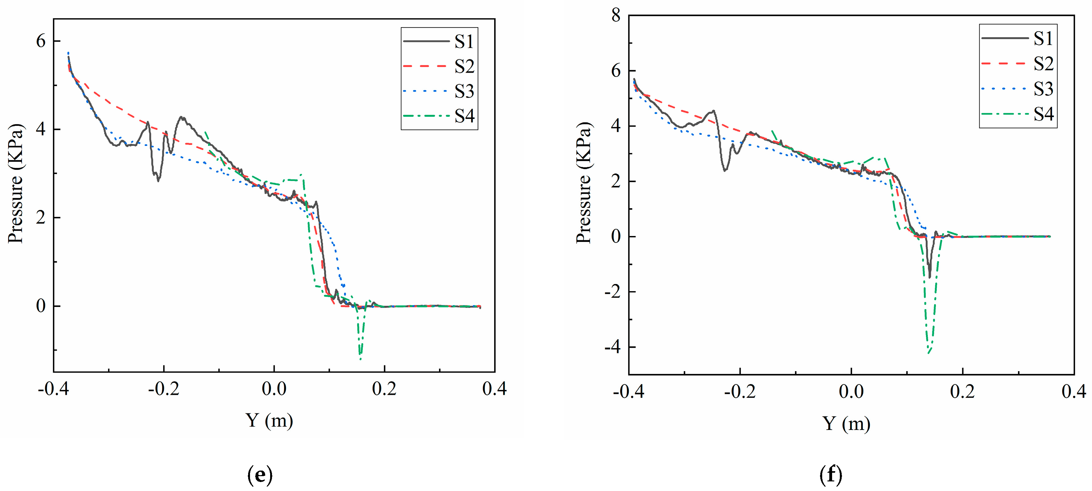
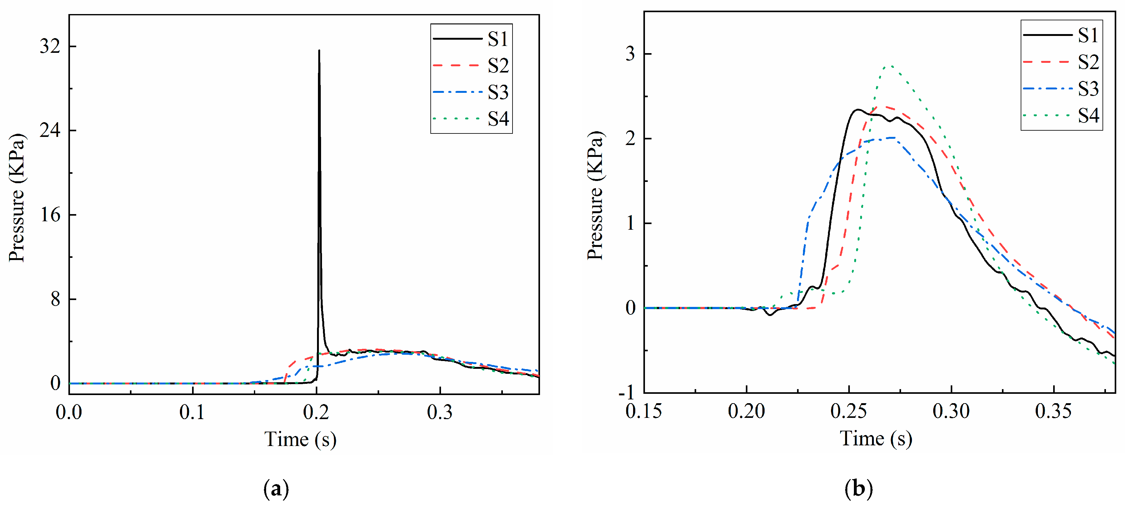
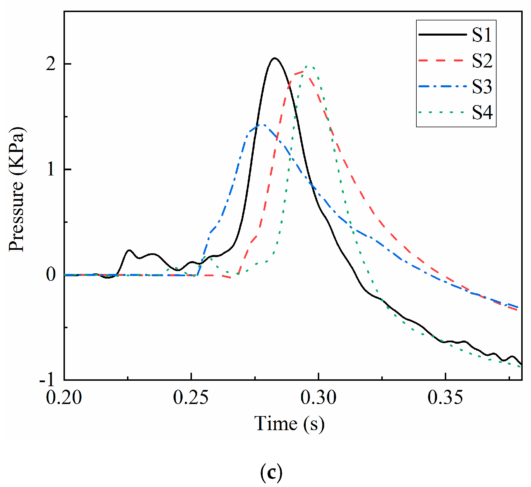
4.2. Pressure Field
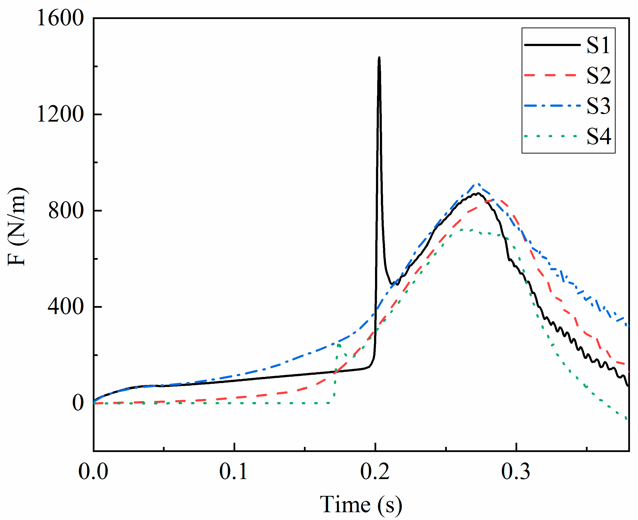
4.3. Impact Force
5. Conclusions
Author Contributions
Funding
Conflicts of Interest
References
- Faltinsen, O.M. Hydrodynamics of High-Speed Marine Vehicles; Cambridge University Press: New York, NY, USA, 2005. [Google Scholar]
- Hirdaris, S.E.; Bai, W.; Dessi, D.; Ergin, A.; Gu, X.; Hermundstad, O.A.; Huijsmans, R.; Iijima, K.; Nielsen, U.D.; Parunov, J.; et al. Loads for use in the design of ships and offshore structures. Ocean Eng. 2014, 78, 131–174. [Google Scholar] [CrossRef]
- Jiao, J.; Ren, H.; Chen, C. Model testing for ship hydroelasticity: A review and future trends. J. Shanghai Jiaotong Univ. (Sci.) 2017, 22, 641–650. [Google Scholar] [CrossRef]
- Jiao, J.; Yu, H.; Chen, C.; Ren, H. Time-domain numerical and segmented model experimental study on ship hydroelastic responses and whipping loads in harsh irregular seaways. Ocean Eng. 2019, 185, 59–81. [Google Scholar] [CrossRef]
- Von Karman, T. The Impact on Seaplane Floats during Landing; NACA Technical Note, No.321; NACA: Ames, IA, USA, 1929. [Google Scholar]
- Wagner, H. Uber Stoss-und Gleitvorgange an der Oberflache von Flussigkeiten. ZAMM 1932, 12, 193–215. [Google Scholar] [CrossRef]
- Zhao, R.; Faltinsen, O.; Aarsnes, J. Water entry of arbitrary two-dimensional sections with and without flow separation. In Proceedings of the 21st Symposium on Naval Hydrodynamics, Trondheim, Norway; National Academy Press: Washington, DC, USA, 1996. [Google Scholar]
- Sun, H.; Faltinsen, O.M. Water entry of a bow-flare ship section with roll angle. J. Mar. Sci. Technol. 2009, 14, 69–79. [Google Scholar] [CrossRef]
- Aarsnes, J. Drop Test with Ship Sections—Effect of Roll Angle; Report 603834.00.01; Norwegian Marine Technology Research Institute: Trondheim, Norway, 1996. [Google Scholar]
- Wang, S.; Guedes Soares, C. Slam induced loads on bow-flared sections with various roll angles. Ocean Eng. 2013, 67, 45–57. [Google Scholar] [CrossRef]
- Yang, L.; Yang, H.; Yan, S.; Ma, Q. Numerical investigation of water-entry problems using IBM method. Int. J. Offshore Pol. Eng. 2017, 27, 152–159. [Google Scholar] [CrossRef]
- Xie, H.; Ren, H.; Li, H.; Tao, K. Numerical prediction of slamming on bow-flared section considering geometrical and kinematic asymmetry. Ocean Eng. 2018, 158, 311–330. [Google Scholar] [CrossRef]
- Yu, P.; Li, H.; Ong, M.C. Numerical study on the water entry of curved wedges. Ships Offshore Struct. 2018, 13, 885–898. [Google Scholar] [CrossRef]
- Panciroli, R.; Shams, A.; Porfiri, M. Experiments on the water entry of curved wedges: High speed imaging and particle image velocimetry. Ocean Eng. 2015, 94, 213–222. [Google Scholar] [CrossRef]
- Chen, Y.; Khabakhpasheva, T.; Maki, K.J.; Korobkin, A. Wedge impact with the influence of ice. Appl. Ocean Res. 2019, 89, 12–22. [Google Scholar] [CrossRef]
- Hermundstad, O.A.; Moan, T. Numerical and experimental analysis of bow flare slamming on a Ro–Ro vessel in regular oblique waves. J. Mar. Sci. Technol. 2005, 10, 105–122. [Google Scholar] [CrossRef]
- Tuitman, J.T.; Bosman, T.N.; Harmsen, E. Local structural response to seakeeping and slamming loads. Mar. Struct. 2013, 33, 214–237. [Google Scholar] [CrossRef]
- Kim, J.H.; Kim, Y.; Yuck, R.H.; Lee, D.Y. Comparison of slamming and whipping loads by fully coupled hydroelastic analysis and experimental measurement. J. Fluids Struct. 2015, 52, 145–165. [Google Scholar] [CrossRef]
- Chen, C.; Huang, C.; Chen, K.; Wang, P. Slamming loads calculation for an oil tanker. In Proceedings of the 33rd International Conference on Ocean, Offshore and Arctic Engineering, San Francisco, CA, USA, 8–13 June 2014. [Google Scholar]
- Seng, S.; Jensen, J.J.; Šime, M. Global hydroelastic model for springing and whipping based on a free-surface CFD code (OpenFOAM). Int. J. Nav. Archit. Ocean Eng. 2014, 6, 1024–1040. [Google Scholar] [CrossRef][Green Version]
- Dhavalikar, S.; Awasare, S.; Joga, R.; Kar, A.R. Whipping response analysis by one way fluid structure interaction—A case study. Ocean Eng. 2015, 103, 10–20. [Google Scholar] [CrossRef]
- Drummen, I.; Holtmann, M. Benchmark study of slamming and whipping. Ocean Eng. 2014, 86, 3–10. [Google Scholar] [CrossRef]
- Takami, T.; Matsui, S.; Oka, M.; Iijima, K. A numerical simulation method for predicting global and local hydroelastic response of a ship based on CFD and FEA coupling. Mar. Struct. 2018, 59, 368–386. [Google Scholar] [CrossRef]
- Bilandi, R.N.; Jamei, S.; Roshan, F.; Azizi, M. Numerical simulation of vertical water impact of asymmetric wedges by using a finite volume method combined with a volume-of-fluid technique. Ocean Eng. 2018, 160, 119–131. [Google Scholar] [CrossRef]
- Krastev, V.K.; Facci, A.L.; Ubertini, S. Asymmetric water impact of a two dimensional wedge: A systematic numerical study with transition to ventilating flow conditions. Ocean Eng. 2018, 147, 386–398. [Google Scholar] [CrossRef]
- Han, F.; Yao, J.; Wang, C.; Zhu, H. Bow Flare Water Entry Impact Prediction and Simulation Based on Moving Particle Semi-Implicit Turbulence Method. Shock Vib. 2018, 2018, 7890892. [Google Scholar] [CrossRef]
- Johannessen, S. Use of CFD to Study Hydrodynamic Loads on Free-Fall Lifeboats in the Impact Phase: A Verification and Validation Study. Master’s Thesis, Norwegian University of Science and Technology, Trondheim, Norway, 2012. [Google Scholar]
- MOERI. Wave Induced Loads on Ships; Technical Report No BSPIS7230-10306-6; Maritime Ocean Engineering Research Institute: Daejeon, Korea, 2013. [Google Scholar]
- Zhao, R.; Faltinsen, O. Water entry of two-dimensional bodies. J. Fluid Mech. 1993, 246, 593–612. [Google Scholar] [CrossRef]


| Case | Minimum Grid Size (m) | Time Step (s) | Total Number of Grids |
|---|---|---|---|
| M1 | 0.005 | 0.001 | 35,476 |
| M2 | 0.0025 | 0.0005 | 125,148 |
| M3 | 0.00125 | 0.00025 | 219,069 |
| M4 | 0.000625 | 0.000125 | 448,163 |
Publisher’s Note: MDPI stays neutral with regard to jurisdictional claims in published maps and institutional affiliations. |
© 2020 by the authors. Licensee MDPI, Basel, Switzerland. This article is an open access article distributed under the terms and conditions of the Creative Commons Attribution (CC BY) license (http://creativecommons.org/licenses/by/4.0/).
Share and Cite
Wang, Q.; Zhang, B.; Yu, P.; Li, G.; Yuan, Z. Numerical Investigation on the Water Entry of Several Different Bow-Flared Sections. Appl. Sci. 2020, 10, 7952. https://doi.org/10.3390/app10227952
Wang Q, Zhang B, Yu P, Li G, Yuan Z. Numerical Investigation on the Water Entry of Several Different Bow-Flared Sections. Applied Sciences. 2020; 10(22):7952. https://doi.org/10.3390/app10227952
Chicago/Turabian StyleWang, Qiang, Boran Zhang, Pengyao Yu, Guangzhao Li, and Zhijiang Yuan. 2020. "Numerical Investigation on the Water Entry of Several Different Bow-Flared Sections" Applied Sciences 10, no. 22: 7952. https://doi.org/10.3390/app10227952
APA StyleWang, Q., Zhang, B., Yu, P., Li, G., & Yuan, Z. (2020). Numerical Investigation on the Water Entry of Several Different Bow-Flared Sections. Applied Sciences, 10(22), 7952. https://doi.org/10.3390/app10227952