Featured Application
The suggested optimization framework may lead to a significant improvement of the 5G urban backhauling network. The suggested technology can simplify the task of upgrading existing metropolitan transport infrastructure to cope with the ever-growing demand for bandwidth enhanced by the 5G technology.
Abstract
This paper presents a set of graph optimization problems related to free-space optical communication networks. Such laser-based wireless networks require a line of sight to enable communication, thus a visibility graph model is used herein. The main objective is to provide connectivity from a communication source point to terminal points through the use of some subset of available intermediate points. To this end, we define a handful of problems that differ mainly in the costs applied to the nodes and/or edges of the graph. These problems should be optimized with respect to cost and performance. The problems at hand are shown to be NP-hard. A generic heuristic based on a genetic algorithm is proposed, followed by a set of simulation experiments that demonstrate the performance of the suggested heuristic method on real-life scenarios. The suggested genetic algorithm is compared with the Euclidean Steiner tree method. Our simulations show that in many settings, especially in dense graphs, the genetic algorithm finds lower-cost solutions than its competitor, while it falls behind in some settings. However, the run-time performance of the genetic algorithm is considerably better in graphs with 1000 nodes or more, being more than twice faster in some settings. We conclude that the suggested heuristic improves run-time performance on large-scale graphs and can handle a wider range of related optimization problems. The simulation results suggest that the 5G urban backbone may benefit significantly from using free-space optical networks.
1. Introduction
Free-space optical (FSO) communication is an optical point-to-point communication technology. This type of model is based on light propagating in free space (air, outer space, or vacuum) for wireless transmission of data.
The FSO communication involves the use of modulated optical or laser beams to send telecommunication information through the atmosphere. The concept of light communication is not new; Alexander Graham Bell first introduced it in 1880. He demonstrated the use of an intensity-modulated optical beam to transmit telephone signals through the air to a distant receiver. Modern FSO commonly makes use of narrow laser beams to maximize the distance and bandwidth; therefore, it also is referred to as “laser-com”. For a general survey on FSO, see in [1].
Unlike radio frequency (RF) communication, FSO requires line of sight (LOS) and therefore is used rarely in urban regions, which typically have limited visibility. However, with the ever-growing demand for bandwidth, FSO technology is gaining increasingly more interest as an alternative to RF communication due to its high bandwidth, high security, flexible networking, and exemption from spectrum licensing [2]. Whereas fixed FSO links between buildings have long been established and form a separate commercial product segment in local and metropolitan area networks, the mobile and long-range applications of this technology have yet to be used. The causes for that lack of use are the vulnerability of FSO links to the fading effect, dispersion and signal obstruction due to weather and atmospheric conditions, and narrow beam width [3].
Therefore, FSO is often addressed as a “best effort” means of communications allowing only 99–99.9% connectivity [4]. Yet, recent FSO devices with 1550 nm technology are less vulnerable to weather and can cope with extreme rain, heavy snow, and significant fog. In fact, modern hi-end FSO devices support 10Gbps links with very high “up-time” of 99.99–99.999% at 150–500 m range [5,6]. Thus, FSO technology can be used as a complementary backbone infrastructure for urban networks.
1.1. Motivation
This work focuses on the challenges of creating urban FSO networks. The suggested adaptive solution is designed as a cost-effective and best-effort algorithm to improve existing urban networks. The need for high-speed cost-effective communication in urban regions is ever-growing as the average communication demands of 4G and 5G users are increasing rapidly. In particular, during the COVID-19 lockdown, the usage of video calls and video-on-demand services increased dramatically [7,8], pushing the overall data throughput to new demand peaks. Motivated by the need for high-speed, cost-effective, and adaptive urban networks, and based on the growing deployment cost of fiber-optic infrastructure, we propose a free-space laser communication network-optimization algorithm. The purpose of such a network is to thicken the existing urban network, which has dynamic needs for internet communication. One example of such dynamic need is the case of a crowded event in which many people upload their photos to social networks. The dynamic nature of urban networks also can be expressed in a daily context, such as when the demand for internet migrates from business centers during the daytime to residential areas at night. The suggested solution allows a flexible and robust optimization of existing urban networks by adding a thin layer of FSO communication.
1.2. Related Works
In recent years, the demand for fast and available communication in urban and rural regions has increased with the rise in the use of social networks and Internet of Things devices. Therefore, a growing research has focused on optimizing communication networks. However, this paper addresses a set of network optimization problems that are relatively new. Shang et al. [9] suggested a dynamic selection of communication facilities for creating connected and full-coverage networks. In their study, they used the bounded-degree nodes, instability link, and labile topology of the FSO model to build an optimization algorithm using a Voronoi diagram. Gu et al. [10] suggested a proactive network reconfiguration algorithm for FSO-based fronthaul and backhaul networks. Their algorithm used mixed-integer nonlinear programming to optimize network power consumption. Those works discussed optimization of data collection from multiple sensors, made possible by the use of small low-voltage transmitters with long-term communications and precise targeting capabilities. In this paper’s research, however, only two conditions are required for FSO network modeling: (1) LOS field restrictions and (2) the cost function over the nodes and FSO links.
The problem of optimizing graphs presented in this work is commonly addressed as a facility location problem (see [11] for a comprehensive research regarding facility location and [12] for a recent survey on multi-criteria location problems). The classic form of this problem is defined on a graph with fixed-weight edges. The goal is to find the optimal solution (a set of vertices) for a set of facilities. A different approach to this classic model addresses the allocation of facilities on a graph with dynamic weights on the edges [13]. In other words, the alternate approach searches for an optimal registration to the graph’s edges, considering all its vertices rather than searching for subsets of optimal vertices. Another related model considers finding a set of minimal vertices in a graph representing antennas on the terrain. That model defines two types of vertices in the graph, representing two types of facilities: base stations (BS) and relay stations (RS). The goal is to find a minimum set of RS that connects all the BS. The motivation for this problem is to minimize the number of antennas that must be deployed on the terrain. This problem was proven to be MAX SNP-hard (i.e., no constant approximation factor) [14]. This paper discusses a related scenario. Instead of using BS and RS, it considers a visibility graph (representing a city map) with potential and demand vertices and weights on the edges and on the vertices.
Another set of problems addressed is the protocol of communication flow from the sink nodes to the leaves on an existing network while supporting longer network life. These flow problems customarily have been used in sensor-based network models where every node has limited energy. Most work on this subject dealt with the question of how to choose proper cluster head (CH) nodes in the network graph. A CH node is responsible for collecting data from the sensors and transmitting it via relay nodes. Traditionally, this problem has been solved by generating stable clusters in the mobile environment, for example, through the lower energy adaptive clustering hierarchy protocol. This grade-routing protocol uses a randomized rotation of local CHs to achieve an even distribution of energy in the network [15]. More recent research has suggested that, in many real-life cases, genetic algorithms (GAs) might lead to improved network performance [16]. In this work, the main purpose is to construct an efficient network in which the data can flow using minimum cost. In other words, instead of choosing the right CH, we want to choose the nodes that best centralize the data transmission in their area. In the network graph, that means finding the right nodes to not only cover an equal area (nodes), but also minimize the cost of this group of nodes.
From the graph theory point of view, the suggested problems discuss algorithms that evolve around edge connectivity, max flow, and a dominating set on a graph. These problems are known to be codependent. For example, computing graph connectivity calls up a max-flow subroutine and is optimized by first finding a proper dominating set. Many heuristic algorithms for finding graph-edge connectivity use max-flow subroutines. Even and Tarjan [17] suggested using such algorithms. Other works, such as those in [18,19,20,21], improved their algorithm complexity to for a graph with n vertices and m edges by finding some small (but not necessarily optimal) dominating set D of the graph G and using amortized complexity on the computation for the vertices of that set. This current work uses those algorithms to build and evaluate solutions for the FSO network-optimization problem. Most theoretical problems described in the previous paragraph have been proven NP-hard, meaning we cannot compute an optimal solution for them in polynomial time. Nevertheless, some heuristic algorithms can provide a close solution in efficient run time.
One common heuristic used for network optimization is GA. Holland proposed this method in 1973 [22] as an evolution-based stochastic optimization algorithm with a global search for generating useful solutions. The GA is an example of a large family of heuristics called evolutionary algorithms. Inspired by biological evolution, they mimic the behavior of population survival. The algorithms are iterative and contain methods inspired by the processes of development, reproduction, selection, and natural selection (according to principles of Charles Darwin’s survival of the fittest theory). This study addresses some network optimization problems induced by the Steiner tree problem for graphs. Given a weighted graph with a subset of vertices S, the Steiner tree problem is to find the minimum-cost subtree that spans all vertices in S [23]. Kapsalis et al. developed a simple implementation for the GA to solve the Steiner tree problem for graphs [24]. The initial population for their algorithm was a random minimum spanning tree (MST) of the original graph and a time limit of 4000 s to reach solution. Their algorithm reached an approximation of 7.3% from the optimal solution. The Euclidean Steiner tree problem is defined as follows. Given n points on the plane, connect all the points by lines of minimum total length in such a way that any two points may be interconnected by line segments either directly or via other points and line segments. For the Euclidean Steiner tree problem, there exists a GA implementation [25].
1.3. Our Contributions
This paper presents a general framework for optimizing FSO urban networks. The ever-growing demand for bandwidth requires frequent upgrading of the transport layer of networks, in particular in dense cities and urban regions. Using FSO for backhauling allows a cost-effective alternative to fiber-optic cables and RF links. FSO requires neither frequency licensing nor performing road construction, which are both expensive and time consuming. Therefore, the use of FSO in urban regions may increase dramatically along with the adaption of 5G technology. In this paper, we present a generic method for optimizing large-scale FSO networks. The suggested heuristic is based on genetic algorithm. Simulation results show that it often outperforms the existing Steiner approximation algorithm [26] as implemented in the Networkx package [27]; the genetic algorithm has better run-time performance on real-world scenarios (above 1000 vertices). Moreover, most importantly, the suggested algorithm is applicable on a wide range of network constrains and problems, while the existing algorithms for the Steiner problem are only applicable for the simplified version of the FSO optimization problem. To the best of our knowledge, this is the first paper that suggests a generic optimization method suitable for solving multi-constraint real-world FSO problems.
2. Problems Statement
This section presents the main optimization problems related to the construction of FSO networks. A core component in any FSO-related problem is the visibility graph [14,28,29], in which a vertex (node) represents a point on the terrain, and an edge represents a link between two points with LOS between them.
Herein, an FSO graph is defined as a visibility graph with red and blue vertices [26].
Next, we present five optimization problems of interest in the context of constructing FSO networks, followed by some required definitions and models:
- Given a visibility graph, find the spanning tree (network) with maximum endpoints (leaves).
- Given an FSO graph, find the network with minimum intermediate points that connects all terminal points.
- Given an FSO graph with positive-weighted vertices, find the network with minimum overall node cost that connects all terminal points.
- Given an FSO graph with positive-weighted edges, find the network with the minimum overall edge cost that connects all terminal points.
- Given an FSO graph with positive-weighted vertices and edges, find the network with the minimum overall (combined node and edge) cost that connects all terminal points.
To formalize the above problems, we define the following preliminaries.
- Terrain: , 2-dimensional (D) function from where is the location on the terrain and z is the height of this point.
- Building P: a 2.5D polygon on the terrain with height from the ground.
- Line of sight: Between two buildings, there is LOS (i.e., visibility) if and only if there is a straight line between them that does not intersect any other building on the terrain.
- City map: Subcase of a terrain that represents an urban canyon (2.5D polygons). In this work, we consider the ground to be flat terrain and the buildings to be of rectangular shape, each with a positive height z from the ground.
- Terminal points, denoted as B: The subset of buildings that require communication (blue vertices).
- Intermediate points, denoted as R: The set of all buildings that are not “blue” and on which a communication facility can be positioned (red vertices).
- Sink (root): A communication source point for the terminal points. In general, there might be a few sinks that, combined, should supply all the city’s communication demands. However, we mainly consider the case of a single source.
- function: FSO communication requires a clear LOS. Two buildings may have an FSO link between them if there is visibility between rooftops and the distance between them is below some maximum value. Thus, we define a binary function if , satisfy the function requirements, , where the function requirements are as follows.
- -
- LOS exists: No third building blocks the LOS between and .
- -
- Distance: The distance between these buildings is not longer than a predefined maximal range.
We now define the main graph model used in this paper, the FSO visibility graph model. The visibility graph is an undirected graph defined by the binary function . The following types of simple graph models enable us to define our problems of interest (Figure 1), demonstrating the visibility graph on a group of buildings.
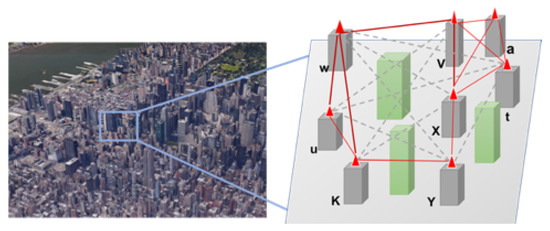
Figure 1.
Visibility graph simulation.
- Let be a visibility graph, which is an undirected graph. This graph is defined by the binary function on a terrain , where each vertex represents a building.
- Let be a red–blue visibility graph. In this graph, B is a set of terminal points and R is a set of intermediate points. The edges in this graph are defined as follows. For every , if and only if , where are the buildings represented by u and v, respectively.
- Let be a , where (all vertices are blue).
- Let be a connected subgraph of where and .
- Valid solution: A network that connects all the terminal points. In other words, a valid solution is a connected graph over the terminal points.
Next, we formally define the problems in focus and discuss their computational complexity (hardness state). We rely on the observation that every regular graph can represent a visibility graph on some terrain and deduce the problem complexities from the regular graph case. For visibility graph complexity analysis, see Section 2.6.
2.1. Network with Maximum Number of Terminal Points
The problem of finding a network with the maximum number of endpoints serves as the baseline problem in this paper. It is motivated by the property of endpoints being less expensive in “real-world” FSO scenarios. This problem is known in the literature as the max-leaf problem.
Definition 1.
For a graph , find a spanning tree with maximum leaves, where a leaf is a vertex with only one adjacent vertex. Figure 2 demonstrates the max-leaf problem on a small graph.
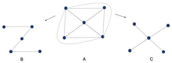
Figure 2.
An example of two different spanning trees of (full graph with 5 nodes). Graph A is , Graph B has only two leaves, and Graph C has the maximum leaf number (four leaves).
The max-leaf problem is known to be NP-hard [30]. There is a polynomial-time algorithm for a graph with maximum degree 3 [31]. In our case, the visibility graph is often dense, and the maximum degree is not bounded by 3. Furthermore, the general max-leaf problem has no polynomial-time approximation scheme, meaning no algorithm can give an infinitely close solution for this problem, assuming . However, there exists a 2-factor approximation in polynomial time for this problem. In this scenario, a solution that contains up to two times the amount of nodes than necessary is not reliable. There is also a solution with reasonable run time for this problem in small graphs of up to 50 nodes [32]. Moreover, such an assumption is inapplicable in many urban visibility graphs.
2.2. Connected Network with Minimum Number of Intermediate Points
This scenario includes some terminal points (blue vertices) in the city that need to be connected and some optional intermediate points (red vertices) that may be used as relays to enable connectivity. This problem is motivated by the need to place new infrastructure at the chosen intermediate points.
Definition 2.
Given a red–blue visibility graph , find a spanning tree that contains all vertices in B and a minimum number of vertices in R. The solution for this problem is a with minimum number of red vertices ( depicts the induced edges of graph ). Figure 3 provides an example of such a problem. Two possible solutions are depicted in Figure 4.
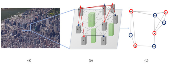
Figure 3.
A simple visibility graph that displays a terrain with a set of (green and gray) buildings: (a) an example of buildings in a “real” city map; (b) an enlarged part of the map, where the red lines represent FSO links between two buildings, and the gray dashed lines are non-FSO links; and (c) the red-–blue visibility graph of the terrain, where each point in the graph corresponds to a building.
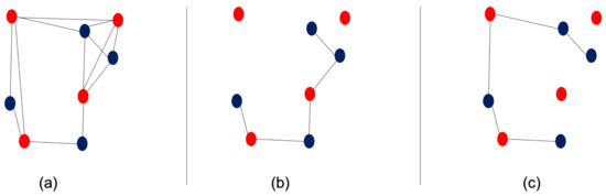
Figure 4.
The visibility and optimal graphs of the example in Figure 3: (a) the visibility graph, (b) an optimal solution, and (c) another optimal solution.
The complexity of this problem (on general graphs) is known to be NP-hard [14].
2.3. Network with Minimum Vertex Cost That Connects All Terminal Points
Here, the previous problem is extended by adding weights to the vertices in the graph. This problem is motivated by the fact that the cost of placing the infrastructure may vary among different intermediate points; for instance, the building owners may demand different payments for using their roofs.
Definition 3.
Given a red–blue visibility graph and a vertex cost function , find a set of vertices of minimal overall cost that connects all the vertices in B. The solution for this problem is a with .
The previous unweighted variant can be reduced to the weighted variant herein by setting all vertex costs to 1. Thus, following the hardness of the unweighted variant [14], the weighted variant is also NP-hard (on general graphs).
2.4. Network with Minimum Edge Cost That Connects All Terminal Points
We now consider a similar problem to the previous, with the difference that costs are applied on edges rather than on vertices. Applying costs on the edges is motivated by the need to place different FSO hardware for different scenarios (e.g., distance or density).
Definition 4.
Given a red–blue visibility graph and an edge cost function , find a set of edges of minimal overall cost that connects all the vertices in B, possibly using some red vertices . The solution for this problem is a with . This problem is also known as the Steiner tree problem for graphs. Note that the problem’s optimal solution is not necessarily a graph that connects all terminal points with the minimum possible number of edges. This is illustrated by the example in Figure 5.
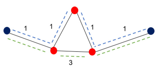
Figure 5.
An example of a red–blue edge-weighted graph. The optimal solution (top blue) uses four edges, which leads to an overall edge cost of 4; terminal connectivity is achievable with just three edges (bottom green), but with a higher edge cost of 5.
The Steiner tree problem for graphs is NP-hard (on general graphs), and its decision variant is known as one of Karp’s 21 NP-complete problems [33]. The problem has a polynomial-time approximation of factor ≈1.39 [34]. Several heuristic algorithms were proposed for this problem throughout the years [26].
2.5. Network with Minimum Combined Vertex and Edge Cost That Connects All Terminal Points
The most general problem we consider applies costs to both vertices and edges. The motivation for this problem is clear: Costs in real-life scenarios may be applied to both vertices (placing infrastructure) and edges (varying required FSO hardware).
Definition 5.
Given a red-blue visibility graph , a vertex cost function , and an edge cost function , find a set of vertices and a set of edges that connect all the vertices in B with minimal combined vertex and edge overall cost. The solution for this problem is a with .
The Steiner tree problem for graphs can be reduced to the general problem herein by settings all vertex costs to zero. Thus, following the hardness of the Steiner tree problem for graphs, the general problem is also NP-hard (on general graphs).
2.6. General Properties of the Visibility Graph
We present a lemma showing the visibility graph model to be as general as a regular undirected graph. As mentioned, the optimization problems of max-leaf and Steiner tree on graphs are NP-hard. In this subsection, we show that every graph can be represented as a visibility graph on some terrain. Moreover, such terrain and its corresponding visibility graphs can be computed efficiently.
Lemma 1.
For any graph , there exists a terrain τ (of size ) and a geometric embedding of V on τ. The visibility graph of over τ is the same graph as G.
Proof.
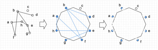
By construction: The visibility graph can be constructed by starting from a null graph, where all the vertices are located on the outer boundary of a thin n-edges polygon. For each two vertices () that are connected in the graph, a narrow “window” (white “segment”) is created between to allow visibility between them without changing the other visibility relations. Such construction has an size, as each additional edge adds two segments to the polygon. The construction is demonstrated in Figure 6. □
Figure 6.
Visibility graph representation on a simplified terrain. Left: a graph. Mid: the vertices are located on a polygon of n edges; the black polygon represents a “wall”. Each edge in the graph is marked as a (blue) segment in the polygon. Right: each visibility segment is marked in white to allow a “visibility window” related to each edge in the graph.
Corollary 1.
The visibility graph model is equivalent to the general undirected graph model.
3. A Genetic Algorithm for FSO Communication Networks
This section presents an algorithm for creating connected FSO networks. As discussed in the previous section, the FSO problems at the focus of this paper are NP-hard. Consequently, there is no known algorithm for computing the optimal network in a reasonable time (for large networks). However, possible solutions for hard problems on graphs can be produced with low run time by applying heuristic methods [24]. The fast computation issue becomes all the more important due to dynamic changes that commonly occur in FSO networks, which are inherently sensitive to changes in climate and demand. For example, an office building may have great demand in the daytime, but most of the demand moves to nearby residential buildings in the evening. Another example is when fog blocks the LOS.
Bio-inspired algorithms are a family of heuristic methods that simulate biological processes that exist in nature, such as the immune system, viral systems, and insect swarms. Evolution is the biological process that inspires GAs, which simulates DNA growth and mutation in cells. Next, we present a GA for solving the FSO problems at hand. The GA consists of a set of solutions, termed population, that iteratively changes for a given number of rounds (generations), after which the most fitting solution is obtained. The algorithm consists of five essential elements:
- Population initialization: This element, which constitutes the first stage of the algorithm, generates a set of possible valid solutions to the problem. This set of solutions is termed the initial population.
- Crossover (merging): This element is an operator that receives as input two possible solutions and creates a new solution that combines the two. The idea is to improve the two solutions by taking valuable features from each (similarly to DNA).
- Mutation: This element adds random changes to each solution. As in the biological process, the mutation operator creates arbitrary changes to a solution. These changes can create a high-grade solution that is unlikely to result from the crossover operator.
- Evaluating solution: This element, often termed the fitness function, grades each solution. The grade determines the solution’s quality, which affects the probability that the solution will survive to the next generation. For example, a fitness function on a weighted graph can be the sum of the edge/vertex weights.
- Selection: This element is in charge of selecting the next generation of solutions according to their fitness score. The new population obtained from the selection process is further evolved by repeating the crossover and mutation steps and so forth.
The basic GA structure is illustrated in Figure 7.
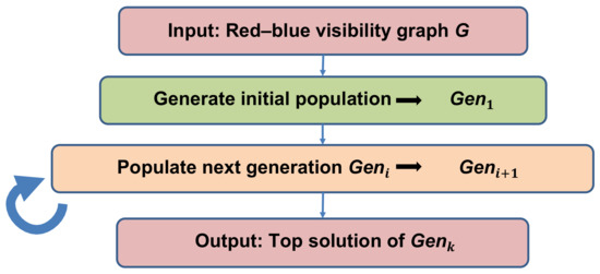
Figure 7.
Basic flow of the genetic algorithm (GA).
The following subsections present a GA that has been specifically designed to solve the described FSO problems.
Before proceeding to the details of the algorithm, we first present some notations:
- Let be the connected component in G that contains vertex v. This can be computed in time, where E is the number of edges in G, by applying the algorithm.
- Let be the shortest path between two vertices and . The shortest path is represented by an ordered set of vertices and edges in a graph. Accordingly, represents the shortest path between vertex and some vertex in the subgraph . In a slight abuse of notation, we denote by the length (number of edges) of the path .
3.1. Generate Initial Population
The first stage of the algorithm is to generate a set of solutions (namely, graphs) that constitutes the first generation (i.e., the initial population). This is an important step because generating high-quality solutions for the initial population can significantly affect the quality of subsequent generations.
The process, described in Algorithm 1, begins with an empty set of solutions (line 1) and an initial graph , which is the induced subgraph of a graph G for vertex subset B (line 2). constitutes the basic graph from which all the k initial solutions are generated.
| Algorithm 1: Pseudocode of , which creates the initial population that consists of k random solutions. |
 |
In most realistic settings , thus is most probably not connected. Therefore, to generate a population of valid solutions, the solutions must be such that all B vertices are connected. To that end, (see Algorithm 2) ensures that a solution is indeed “blue-connected” by invoking a stochastic process that commences from the sink s (Algorithm 1, line 4). Such a mode of operation enables adding k valid and possibly different solutions to the initial population (lines 3–6).
Figure 8 illustrates the creation of two valid initial solutions.
| Algorithm 2: Pseudocode of , which iteratively adds blue vertices and connects them to the graph until a valid solution is obtained. |
 |
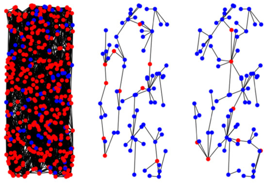
Figure 8.
Example of valid random solutions. The left side of the figure shows an example red–blue visibility graph, whereas two different valid solutions are depicted to its right.
The process, presented in Algorithm 2, is a core ingredient in the GA scheme proposed herein. It is invoked in the generation of not only the initial population, but also subsequent generations, so as to validate solutions after the and operations (explained in the next subsections). Thus, is designed to be robust and fast. It starts with , which is the connected component in that contains the sink vertex s (Algorithm 2, line 1). Next, the connected component is iteratively extended until it contains all the blue vertices (lines 2–6). Each such iteration consists of three steps: (1) choose a blue vertex v that is currently not in (line 3), (2) find a random path to this vertex from (line 4), and (3) update (line 5). The first two steps are random, which enables generating different solutions. A more elaborate discussion on these three steps is given after the following observation.
Observation 1.
The original graph G (including all red vertices) is connected, and stops only when contains all of the blue vertices. Each new vertex added to maintains the connectivity of . Therefore, each solution created by is valid.
Once a new blue vertex is selected, it needs to be connected to . Algorithm 3 describes the process of adding the path to that vertex. For the sake of randomness, a relay vertex is chosen, through which the path to v shall pass. However, this may lead to long and inefficient paths and eventually to poor solutions when a distant vertex (from the shortest path between v and the connected component ) is chosen instead of other more appropriate relay vertices. Thus, only vertices that lead to a path at most d hops long () are considered (Algorithm 3, lines 1 and 3). Ultimately, a relay vertex is randomly chosen from the set of valid options (line 6), and the resulting (shortest) path P that goes through is returned (lines 7–8). Finally, the path P is added to the graph (Algorithm 2, line 5).
| Algorithm 3: Pseudocode of , which finds a random path connecting a new vertex to a graph. |
 |
Figure 9 illustrates the randomness of by showing two possible ways to connect a new vertex v.
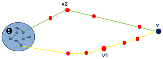
Figure 9.
Illustration of two possible paths for connecting the blue vertex v to the component of the sink vertex s, one through relay vertex , and another through relay vertex .
The above constitutes a constructive process of gradually adding vertices (and the paths that connect them) to the connected component of the sink vertex s until a valid solution is obtained. Another possible approach is to apply a destructive process, in which red vertices are gradually removed from the initial graph G, as long as the graph remains valid (i.e., “blue-connected”). In real-world FSO applications, there are commonly many more red vertices than blue ones; thus, the constructive approach has been chosen herein.
The process is used not only in , but also in the construction of subsequent generations to ensure the validity of obtained solutions.
3.2. Creating the Next Generation
Evolutionary algorithmic schemes such as GA simulate the change of population by creating generations of solutions. The formation of each new generation in the GA herein is performed by a process called nextGeneration. The goal of this process is to create increasingly stronger solutions in every round (generation) by attempting to produce strong new solutions that are based on solutions from the previous generation and on eliminating weak solutions. New solutions are obtained by invoking the and operators. Subsequently, the function evaluates the quality of these newly obtained solutions. Finally, the new generation’s population is selected according to the calculated fitness scores of the obtained solutions. The iterative flow of nextGeneration is depicted in Figure 10.
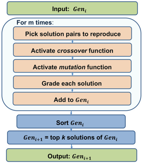
Figure 10.
The iterative flow of nextGeneration.
Denote by the popuation of solutions of the current generation i. The population of the next generation is a set of solutions with the following attributes; (1) ; (2) will contain solutions from with the addition of new solutions obtained by using the and operators; (3) to obtain “strong” genes, the resulting k most-fit solutions will be chosen for . Algorithm 4 presents the pseudocode of the nextGeneration process.
| Algorithm 4: Pseudocode of nextGeneration, which creates the population of the next generation by applying the and operators on solutions from the previous generation. The new population consists of the k “best” obtained solutions. |
 |
Observation 2.
The quality of solutions can only improve from generation to generation.
The above observation holds because all the m newly obtained solutions through and join the k original solutions of the current generation , before the next generation is formed from the top k solutions (of the possible solutions). Consequently, in the worst case, all newly obtained solutions are “worse” than the original k solutions of , leading to . Otherwise, the population is strictly better than . The observation makes the present GA an “anytime” algorithm [35], which is a key feature for heuristic algorithms.
The process is invoked for a given number of times, according to the predefined number of generations (see Figure 7). Nevertheless, the anytime feature enables deciding at any point whether to continue the process or settle for the current best solution without the risk of ending up with some temporary bad solution.
3.3. Crossover Operator
The crossover operator produces new solutions for the next generation. It takes two solutions (graphs) and produces a new solution that is a combination of them. The crossover operator receives two valid red–blue visibility graphs , and outputs a new graph that is also valid (i.e., “blue-connected”). The GA activates the crossover operator repeatedly; thus, it needs to be computed quickly. The crossover operator is formally described in Algorithm 5.
In line 1, the red vertices of the two input subgraphs are intersected to obtain the set of mutual red vertices . Such an operation of combining the two inputs is the essence of the crossover because it preserves the “genetic” attributes of the parents’ “genes”. Next, the blue vertices are added to obtain (line 2) before devising , which is the induced subgraph of G (For ease of presentation, the original graph G and the sink vertex s are omitted as inputs in Algorithms 5 and 6.) with the vertices (line 3).
| Algorithm 5: Pseudocode of the operator. |
 |
| Algorithm 6: Pseudocode of the operator. |
| Input: A connected red–blue visibility graph . |
| Result: A mutated connected red–blue visibility subgraph . |
| randomly choose |
| remove v from |
| return |
Note that most red vertices in and are essential for the respective connectivity of and . Therefore, the resulting graph after the crossover is most probably not “blue-connected”. Such a phenomenon is exemplified in Figure 11. If this is the case, then is applied to ensure that is a valid solution (line 5) before it is returned in line 7.
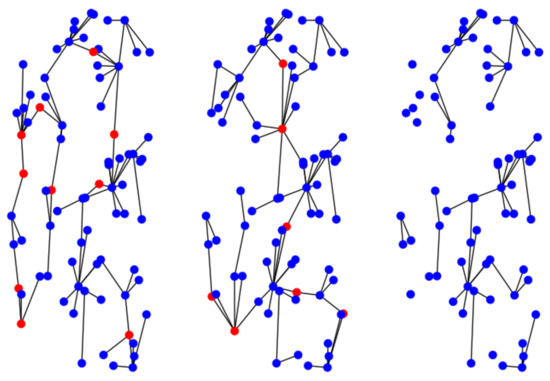
Figure 11.
Example of an invalid crossover. The right graph is the result of a crossover between the two left graphs without applying .
3.4. Mutation Operator
The operator adds variance to the solutions. It is activated on the solutions immediately after their creation (through ). The operator, presented in Algorithm 6, is motivated by the DNA genetic-mutation effect and is probabilistic in a similar manner.
The mutation is implemented by replacing a randomly selected vertex v (Algorithm 6, lines 1–2) with other randomly selected vertex(ices). This is achieved by invoking (line 3), which is both random and fast. Such a mode of operation ensures that the solution , returned in line 4, is valid.
3.5. Fitness (Grade) Function
After changes are applied to solution graphs (through and ), the GA needs to re-evaluate their grades to pass the “best” solutions to the next generation (see Algorithm 4, lines 5–9). The GA literature commonly terms this calculation as the function.
In this paper, the function corresponds to the cost of the graph according to the specific problem at hand (as defined in Section 2). This makes the presented GA rather general because it can be adapted to solve any problem in Section 2.2 through Section 2.5. For instance, in case the combined vertex and edge cost is of interest (see Section 2.5), the fitness (grade) of a graph would be
4. Results
This section presents the experiments conducted to evaluate the suggested GA optimization framework by modeling large-scale urban visibility graphs and solving the underlying FSO optimization problems using simulation. This section reviews the tools used to implement the visibility graph model presented in Section 2. The GA and implementation discussed in Section 3 are also presented here, followed by the algorithm results on randomly generated graphs and real-world-data graphs.
4.1. Simulation Framework
To simulate large-scale visibility graphs efficiently and realistically, the Networkx library tool was used in Python. This library contains a wide range of graph types, among them simple graphs, random graphs, geometric graphs, and weighted graphs. The Networkx package also includes common algorithmic implementations [27]. One example is the implementation of the 2-factor approximation method to the Steiner problem. This research deals with facility-location problems in urban regions. To test the heuristic methods presented in this study, we used the Open Street Map (OSM) platform, an open source geo-database that holds urban information [36]. From this database, we extracted information essential for building visibility graphs on a city terrain, such as building locations and heights.
Figure 12 presents a 3D representation of OSM, from which we were able to construct the visibility graph.
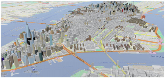
Figure 12.
A 3D map of Manhattan Island, as defined in Open Street Map (OSM). Each building is stored as a 3D shape, allowing us to compute the associated visibility graph.
The visibility graphs were constructed using two main methods: (1) generating random visibility graphs and (2) constructing visibility graphs based on urban data (e.g., open street maps).
All the experiments were run on an Apple MacBook Air with Intel Core i7 processor (quad-core).
4.1.1. Generating a Random Visibility Graph
The first part of the simulation implements a generator for random red–blue visibility graphs. This generator randomly creates graphs while controlling statistical attributes. The importance of such a graph generator is its ability to produce large numbers of graphs while controlling essential parameters, such as edge density and average graph sizes. These graphs were the basis for a variety of experiments.
The random graphs we generated vary in two primary parameters:
- Graph size (number of vertices).
- Graph density (derived from the maximal range capabilities of the FSO links).
The graph size is a key parameter for evaluating the scalability of the algorithm. The number of edges in a graph is also an important parameter to consider, as it significantly affects the algorithm’s performance; thus, we also consider the graph density, which is defined by the following formula,
where m is the number of edges and n is the number of vertices in graph G.
Figure 13 shows example random red–blue visibility graphs. Those examples represent a red–blue graph with different densities, sizes, and red–blue node ratios.
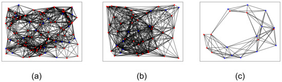
Figure 13.
Three examples of random red–blue visibility graphs. Graph (a) has 100 nodes and edge density. Graph (b) has 50 nodes and edge density. Graph (c) has only 20 nodes, which is useful for quickly testing the algorithms.
In addition to creating random red–blue visibility graphs, we modeled a city terrain in this simulator. The city model has objects representing buildings, building attributes (such as height, location, and shape), and city terrain. On top of this model, we implemented the LOS function (presented in Section 2) and created an LOS geometric-based visibility graph.
4.1.2. Constructing the Visibility Graph Based on Urban Data
The second part of the simulation tests the algorithm on real urban data. Using real urban information modeled as a graph assists in statistical analysis of the city graphs and improvement of the GA. Figure 14 presents an example of such a visibility graph based on urban data of Manhattan Island, from which we took approximately 2000 buildings and 2500 edges; this map is based on OSM.
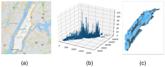
Figure 14.
Manhattan Island visibility graph: (a) a map of Manhattan Island in New York, (b) a chart of all the buildings in that map (using OSM); and (c) the building visibility graph.
4.2. Genetic Algorithm Experiments
This subsection discusses the run time for various graph sizes with different densities and the improvement over time of the algorithm compared to other known methods. The GA was implemented using several Networkx library methods, for example, Dijkstra’s shortest path algorithm.
The experiments for testing the GA is comprised of two parts: (1) comparing the GA to a competing method for solving the Steiner problem and (2) checking the algorithm’s run time and cost improvement over time. These experiments are described next.
4.2.1. Comparison with Other Heuristics
The performance of the GA on the Steiner problem was compared to a standard 2-factor approximation method. The Networkx library has an implementation of the 2-factor approximation method, and we used it in our experiments. Figure 15 demonstrates the solutions of the 2-factor method and the GA on an example graph with 10 vertices.
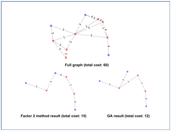
Figure 15.
Two methods comparison example. The full red–blue visibility graph (top) has a total cost of 60. The resulting graphs of the 2-factor (bottom left) method and the GA method (bottom right) have total costs of 15 and 12, respectively.
For the experiments herein, we generated random graphs with different densities and tested both the GA and the 2-factor approximation method on those graphs. The methods were tested for run-time performance and optimal cost. In the first set of experiments, we tested small graphs with 200 vertices and large graphs with 2000 vertices. For each graph size, we tested different densities. Figure 16 and Figure 17 show the run-time performances of the two methods. The larger setting is limited to graphs with only 2000 vertices due to the run-time restrictions of the 2-factor method. As shown in Figure 17, the GA method exhibits better run time on the graphs with 2000 vertices. This is because the 2-factor method builds and searches over a complete graph (with 2000 vertices), whereas the GA searches for the shortest path in the original graph only, when creating the initial population. Further, in the crossover function, the GA searches for the shortest path in much smaller graphs (the union between the trees). This may have low impact on the run time in small graphs (Figure 16) but is very significant as the graphs become larger (Figure 17).
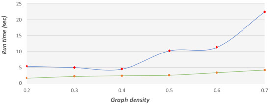
Figure 16.
Run time comparison on graphs with 200 vertices at different densities. This graph presents the run time of the 2-factor approximation method (green) and the GA (blue).
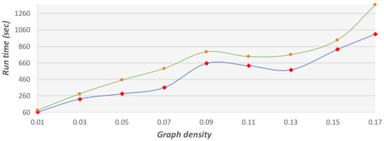
Figure 17.
Run time comparison on graphs with 2000 vertices at different densities. This graph presents the run time of the 2-factor approximation method (green) and the GA (blue).
Figure 18 and Figure 19 present the resulting average cost difference between the GA and the 2-factor approximation method. A negative cost difference means that the GA finds better (lower-cost) solutions than the 2-factor approximation method. Regions in which the 2-factor approximation method finds better solutions than the GA are colored in blue. Evidently, the GA method finds, on average, better solutions than the 2-factor approximation method on both sparse and dense problems, except for the intermediate blue regions. In urban cases, the graphs are expected to be dense (denser when the city is small, and sparser when the city is large). Therefore, the GA can be efficient for urban graphs. The fact that this algorithm is also faster makes it the preferable method for solving Steiner problems on urban graphs.
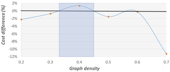
Figure 18.
Cost difference comparison on graphs with 200 vertices at different densities. This graph presents the average cost difference between the GA’s solutions and those of the 2-factor approximation method, which are marked by the fixed black line. The blue region represents graph densities in which the 2-factor approximation method finds better solutions.
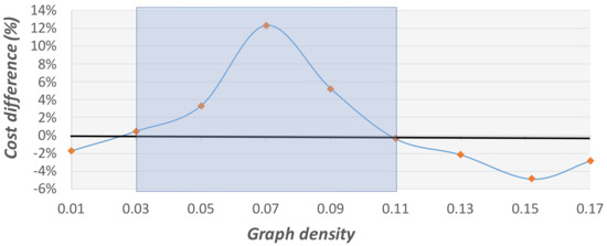
Figure 19.
Cost difference comparison on graphs with 2000 vertices at different densities. This graph presents the average cost difference between the solutions of the GA and those of the 2-factor approximation method, which are marked by the fixed black line. The blue region represents graph densities in which the 2-factor approximation method finds better solutions.
In an additional set of experiments we tested the performance of the two methods on different size graphs with fixed density (0.15). Figure 20 and Figure 21 show the run time comparison and the differences in solution cost, respectively.
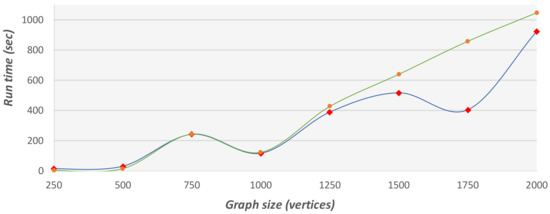
Figure 20.
Run time comparison on graphs with different sizes and 0.15 density. This graph presents the run time of the 2-factor approximation method (green) and the GA (blue).
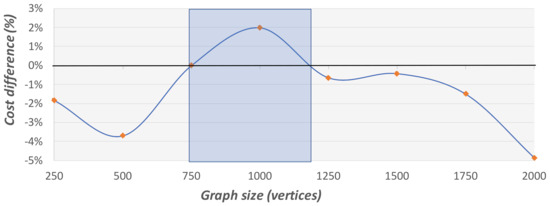
Figure 21.
Cost difference comparison on graphs with different sizes and 0.15 density. This graph presents the average cost difference between the solutions of the GA and those of the 2-factor approximation method, which are marked by the fixed black line. The blue region represents graph sizes in which the 2-factor approximation method finds better solutions.
As these experiments show, the GA is more efficient in terms of run time and solution cost on larger graphs. This confirms that the GA method is more suitable for urban visibility graphs, which are usually very large.
4.2.2. Run Time and Solution Quality
To evaluate the algorithm’s performance, we generated red–blue visibility graphs in several variations with different graph sizes and densities. Additionally, we conducted experiments to optimize the algorithm’s parameters:
- Number of generations.
- Number of crossovers in each generation.
- Mutation probability.
Our experiments show that the optimal formulas for deciding the initial GA parameters (number of crossovers) is
where n is the number of vertices and is computed according to Equation (2).
The mutation function is designed to avoid a local minimum state. Although the function can add variance to the solution pool, this function is not efficient in terms of run time because it searches for the shortest path in the full graph. In the following set of experiments, we activated the mutation function at a probability of 0.01. After fixing the parameters, we tested large graphs for run time and convergence. Figure 22, Figure 23 and Figure 24 show the expected run time of the GA method on graphs with 4000 to 16,000 vertices.
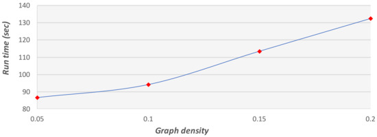
Figure 22.
Run time of the GA on graphs with 4000 vertices at different densities.
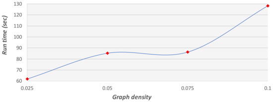
Figure 23.
Run time of the GA on graphs with 8000 vertices at different densities.
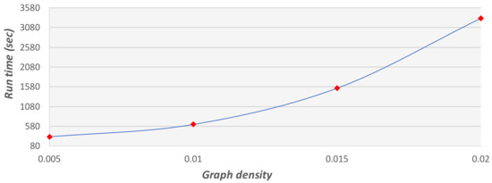
Figure 24.
Run time of the GA on graphs with 16,000 vertices at different densities.
The experiments show that the run time of the GA is strongly connected to the graph density. As the density grows, the run time increases. This is because the main method in our algorithm is the shortest path method. This method (using Dijkstra’s algorithm) searches over all the edges in the graph, and the number of times it is activated is proportional to the graph density.
Next, we tested the algorithm’s ability to improve over generations. Figure 25 demonstrates the algorithm’s cost reduction over 60 generations on an example graph with 2000 vertices. Figure 26 presents the case of another example graph, in which a significant cost reduction occurs after 580 generations, following a long period of stable generations. The latter example suggests that in some situations it is worthwhile to run the GA for many generations. However, we observed empirically that, in most cases, the GA converges in less than 100 generations.
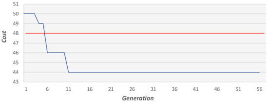
Figure 25.
The cost reduction of the GA over 60 generations on an example problem. The fixed red line represents the result of the 2-factor approximation method.
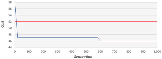
Figure 26.
The cost reduction of the GA over 1000 generations on an example problem. The fixed red line represents the result of the 2-factor approximation method.
Table 1 shows the cost reduction of the GA on large graphs with different densities. The cost reduction relates to the difference (in percents) between the GA’s final solution and the initial (random) solution.

Table 1.
Cost reduction on large graphs with different densities.
4.3. Results on Real-World Data
Now, we present experimental results of the GA on real-world data. Here, we used the OSM open project data to create visibility graphs based on real building coordinates and LOS computation. The framework built for these experiments comprises of three steps:
- Get urban data (location of high buildings in a city).
- Compute the city visibility graph (mainly the LOS between the buildings).
- Compute the Steiner graph with GA and the 2-factor approximation method.
In these experiments, we used the urban data of Manhattan Island in New York City. Figure 27 and Figure 28 show the results on real-world data in the form of histograms. The experiments were run on 100 urban graphs, each with 2000 vertices, of which 5 are blue (i.e., require communication).
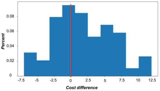
Figure 27.
Cost differences histogram. This histogram demonstrates the cost differences between the GA’s solutions and those of the 2-factor approximation method, which are denoted by the red line. Positive values represent a better (lower) solution cost of the GA.
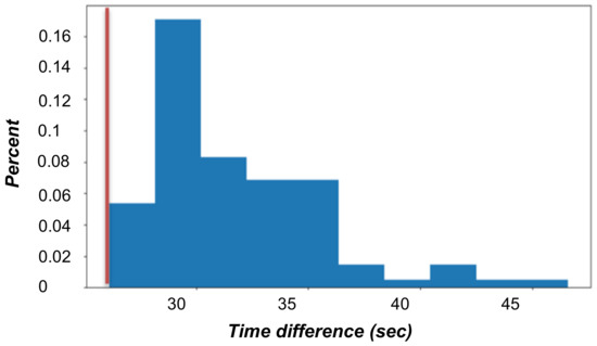
Figure 28.
Time differences histogram. This histogram demonstrates the differences in run time between the GA and the 2-factor approximation method, which are denoted by the red line. Positive values represent better (faster) run time of the GA.
The histogram in Figure 27 shows that the GA does not always return the best solution. However, in most cases, the GA returns better solutions than the 2-factor approximation method. Moreover, the cost differences in favor of the GA tend to be higher than those in favor of the 2-factor approximation method. The histogram in Figure 28 reveals the clear superiority of the GA in run time over the 2-factor approximation method.
We also report a series of experiments that we conducted on large-scale graphs (over 4000 vertices). The graphs were generated randomly, but the graph features (such as density and size) were fixed to simulate urban visibility graphs. From the results, we can conclude that for finding a solution to the Steiner problem on these graphs, the GA was efficient and within a reasonable run time. Because the Steiner problem is NP-hard, we could not test the GA method against the 2-factor approximation method (which demands run time). However, the experiments did show that the GA can reach solutions with up to cost reduction. This fact shows that the algorithm is more efficient than simply choosing a solution at random. Another feature of the GA method is the ability to produce “anytime” solutions, meaning we can decide when to stop the algorithm’s run and get a solution. Given that running the GA on large graphs can take up to 1500 s, this anytime feature becomes especially helpful in dynamic conditions when weather or demand changes affect the urban network.
5. Discussion and Conclusions
This paper presents a new method for the urban FSO network optimization problem. The method uses the Genetic Algorithm (GA) approach to find a connected graph among the network components (which represent buildings in the city). Until recently, FSO technology was not commonly used as a backbone urban network, mainly due to the vulnerability of the laser communication technology to extreme weather conditions. Yet, recent improvements in FSO technology has pushed the expected availability (“up-time”) of FSO networks from [99–99.9]% to [99.99–99.999]% (from 2–3, 9’s to 4–5, 9’s) [4,37] allowing the FSO technology to reach service standards required by the urban infrastructure. Thus, the use of FSO in cost-effective 5G networks is expected to increase [37]. The suggested algorithm can be used for both the initial optimal design of an FSO network and for upgrading (adapting) existing FSO network to changes in the network demands and weather conditions. The suggested GA method is designed to create a solution for a variety of problems regarding the minimization of the facilities and infrastructures in urban FSO networks. The algorithm’s advantage is considered in two main factors: run time and the “anytime” feature.
As our experiments show, the GA method has no run-time advantage on relatively small (200 vertices) graphs. However, as the graphs increase in size, our method gains a significant advantage over other methods for calculating the Steiner graph. In addition, after correctly setting the algorithm parameters, it appears that the GA can find high-quality solutions. This advantage can be seen in both the random graphs and the real-world graphs examined. The algorithm is shown to have improved performance on visibility graphs representing real cases of urban information (with relatively high density). Based on these results, and because the algorithm is generic for several problems other than the Steiner problem, we can determine that the algorithm proposed here is suitable for finding relatively low-cost networks on urban FSO graphs.
We also observed that the suggested algorithm for finding a connected graph could be generalized to the generic multi-source case. Consider the case of a large city with several internet gateways (a set S of sources). The multi-source problem is defined as follows. Given a graph and a set (representing the sources), find a subgraph , in which each vertex in is connected to one of the vertices in S.
Observation 3.
Let be the graph G with additional edges that connect all the sources. Applying the GA on will imply a valid (multi-source) solution over G. Figure 29 demonstrates a GA solution on a multi-source graph.
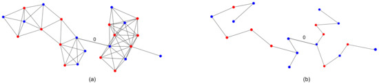
Figure 29.
Multi-source graph example. Graph (a) is a full red–blue visibility graph comprised of two subgraphs with a single connecting edge (with weight 0). Graph (b) is the GA result for graph (a). Note that because we artificially connected two subgraphs with a single edge of weight 0, we can run the algorithm on each subgraph separately and achieve the same result.
For future work, we plan to examine whether the suggested methods can be expanded to dynamic networks with adaptive weights (costs) on the edges. Another possible generalization of the model is to construct robust two-connectivity solution.
Author Contributions
This research was equally contributed by all three authors: R.M., B.B.-M., and T.G. Conceptualization, B.B.-M. and R.M.; methodology, T.G.; software, R.M.; validation, B.B.-M., T.G. and R.M.; formal analysis, T.G.; data curation, R.M.; writing—original draft preparation, B.B.-M., T.G., and R.M.; writing—review and editing, T.G.; visualization, R.M.; All authors have read and agreed to the published version of the manuscript.
Funding
This work was partially supported by the Ariel Cyber Innovation Center in conjunction with the Israel National Cyber Directorate in the Prime Minister’s Office.
Conflicts of Interest
The authors declare no conflict of interest.
References
- Killinger, D. Free space optics for laser communication through the air. Opt. Photonics News 2002, 13, 36–42. [Google Scholar] [CrossRef]
- Henniger, H.; Wilfert, O. An Introduction to Free-space Optical Communications. Radioengineering 2010, 19, 203–212. [Google Scholar]
- Nadeem, F.; Kvicera, V.; Awan, M.S.; Leitgeb, E.; Muhammad, S.S.; Kandus, G. Weather effects on hybrid FSO/RF communication link. IEEE J. Sel. Areas Commun. 2009, 27, 1687–1697. [Google Scholar] [CrossRef]
- Bloom, S.; Korevaar, E.; Schuster, J.; Willebrand, H. Understanding the performance of free-space optics. J. Opt. Netw. 2003, 2, 178–200. [Google Scholar] [CrossRef]
- Kim, I.I.; Korevaar, E.J. Availability of free-space optics (FSO) and hybrid FSO/RF systems. In Proceedings of the Optical Wireless Communications IV. International Society for Optics and Photonics, Denver, CO, USA, 14–16 December 2001; Volume 4530, pp. 84–95. [Google Scholar]
- Singh, H.; Chechi, D.P. Performance Evaluation of Free Space Optical (FSO) Communication Link: Effects of Rain, Snow and Fog. In Proceedings of the 2019 6th International Conference on Signal Processing and Integrated Networks (SPIN), Noida, India, 7–8 March 2019; pp. 387–390. [Google Scholar]
- Bary, E. Zoom, Microsoft Teams Usage Are Rocketing during Coronavirus Pandemic. 2020. Available online: https://www.marketwatch.com/story/zoom-microsoft-cloud-usage-are-rocketing-during-coronavirus-pandemic-new-data-show-2020-03-30 (accessed on 15 September 2020).
- News, B. Netflix Gets 16 Million New Sign-Ups Thanks to Lockdown. BBC, 22 April 2020. [Google Scholar]
- Shang, T.; Zhao, P.; Gao, Y.; Liu, Y. Research on topology control based on Voronoi diagram algorithm in FSO networks. Telecommun. Syst. 2019, 72, 81–93. [Google Scholar] [CrossRef]
- Gu, Z.; Zhang, J.; Ji, Y.; Bai, L.; Sun, X. Network topology reconfiguration for FSO-based fronthaul/backhaul in 5G+ wireless networks. IEEE Access 2018, 6, 69426–69437. [Google Scholar] [CrossRef]
- Drezner, Z.; Hamacher, H.W. Facility Location: Applications and Theory; Springer Science & Business Media: Berlin/Heidelberg, Germany, 2001. [Google Scholar]
- Farahani, R.Z.; SteadieSeifi, M.; Asgari, N. Multiple criteria facility location problems: A survey. Appl. Math. Model. 2010, 34, 1689–1709. [Google Scholar] [CrossRef]
- Ben-Moshe, B.; Elkin, M.; Gottlieb, L.A.; Omri, E. Optimizing budget allocation in graphs. arXiv 2014, arXiv:1406.2107. [Google Scholar]
- Ben-Shimol, Y.; Ben-Moshe, B.; Ben-Yehezkel, Y.; Dvir, A.; Segal, M. Automated antenna positioning algorithms for wireless fixed-access networks. J. Heuristics 2007, 13, 243–263. [Google Scholar] [CrossRef]
- Heinzelman, W.R.; Chandrakasan, A.; Balakrishnan, H. Energy-efficient communication protocol for wireless microsensor networks. In Proceedings of the 33rd Annual Hawaii International Conference on System Sciences, Maui, HI, USA, 7 January 2000; p. 10. [Google Scholar]
- Bhatia, T.; Kansal, S.; Goel, S.; Verma, A. A genetic algorithm based distance-aware routing protocol for wireless sensor networks. Comput. Electr. Eng. 2016, 56, 441–455. [Google Scholar] [CrossRef]
- Even, S.; Tarjan, R.E. Network flow and testing graph connectivity. SIAM J. Comput. 1975, 4, 507–518. [Google Scholar] [CrossRef]
- Schnorr, C.P. Bottlenecks and edge connectivity in unsymmetrical networks. SIAM J. Comput. 1979, 8, 265–274. [Google Scholar] [CrossRef]
- Galil, Z. Finding the vertex connectivity of graphs. SIAM J. Comput. 1980, 9, 197–199. [Google Scholar] [CrossRef]
- Galil, Z.; Italiano, G.F. Reducing edge connectivity to vertex connectivity. ACM Sigact News 1991, 22, 57–61. [Google Scholar] [CrossRef]
- Matula, D.W. Determining edge connectivity in 0 (nm). In Proceedings of the 28th Annual Symposium on Foundations of Computer Science, Los Angeles, CA, USA, 12–14 October 1987; pp. 249–251. [Google Scholar]
- Holland, J.H. Genetic algorithms and the optimal allocation of trials. SIAM J. Comput. 1973, 2, 88–105. [Google Scholar] [CrossRef]
- Gilbert, E.N.; Pollak, H.O. Steiner minimal trees. SIAM J. Appl. Math. 1968, 16, 1–29. [Google Scholar] [CrossRef]
- Kapsalis, A.; Raywad-Smith, V.; Smith, G.D. Solving the graphical Steiner tree problem using genetic algorithms. J. Oper. Res. Soc. 1993, 44, 397–406. [Google Scholar] [CrossRef]
- Hesser, J.; Männer, R.; Stucky, O. On Steiner trees and genetic algorithms. In Workshop on Parallel Processing: Logic, Organization, and Technology; Springer: Berlin/Heidelberg, Germany, 1989; pp. 509–525. [Google Scholar]
- Duin, C.; Voß, S. Steiner tree heuristics—A survey. In Operations Research Proceedings 1993; Springer: Berlin/Heidelberg, Germany, 1994; pp. 485–496. [Google Scholar]
- Hagberg, A.; Schult, D.; Swart, P. Networkx: Python software for the analysis of networks. In Mathematical Modeling and Analysis; Los Alamos National Laboratory: Los Alamos, NM, USA, 2005. [Google Scholar]
- Floriani, L.; Magillo, P. Algorithms for visibility computation on terrains: A survey. Environ. Plan. Plan. Des. 2003, 30, 709–728. [Google Scholar] [CrossRef]
- De Floriani, L.; Marzano, P.; Puppo, E. Line-of-sight communication on terrain models. Int. J. Geogr. Inf. Syst. 1994, 8, 329–342. [Google Scholar] [CrossRef]
- Garey, M.R.; Johnson, D.S. Computers and Intractability; Freeman: San Francisco, CA, USA, 1979; Volume 174. [Google Scholar]
- Ueno, S.; Kajitani, Y.; Gotoh, S. On the nonseparating independent set problem and feedback set problem for graphs with no vertex degree exceeding three. Discret. Math. 1988, 72, 355–360. [Google Scholar] [CrossRef]
- Michael, R.F.; McCartin, C.; Frances, A.R.; Stege, U. Coordinatized kernels and catalytic reductions: An improved FPT algorithm for max leaf spanning tree and other problems. In International Conference on Foundations of Software Technology and Theoretical Computer Science; Springer: Berlin/Heidelberg, Germany, 2000; pp. 240–251. [Google Scholar]
- Karp, R.M. Reducibility among combinatorial problems. In Complexity of Computer Computations; Springer: Berlin/Heidelberg, Germany, 1972; pp. 85–103. [Google Scholar]
- Byrka, J.; Grandoni, F.; Rothvoss, T.; Sanità, L. Steiner tree approximation via iterative randomized rounding. J. ACM 2013, 60, 1–33. [Google Scholar] [CrossRef]
- Zilberstein, S. Using anytime algorithms in intelligent systems. AI Mag. 1996, 17, 73. [Google Scholar]
- Haklay, M.; Weber, P. Openstreetmap: User-generated street maps. IEEE Pervasive Comput. 2008, 7, 12–18. [Google Scholar] [CrossRef]
- Alzenad, M.; Shakir, M.Z.; Yanikomeroglu, H.; Alouini, M.S. FSO-based vertical backhaul/fronthaul framework for 5G+ wireless networks. IEEE Commun. Mag. 2018, 56, 218–224. [Google Scholar] [CrossRef]
Publisher’s Note: MDPI stays neutral with regard to jurisdictional claims in published maps and institutional affiliations. |
© 2020 by the authors. Licensee MDPI, Basel, Switzerland. This article is an open access article distributed under the terms and conditions of the Creative Commons Attribution (CC BY) license (http://creativecommons.org/licenses/by/4.0/).