Visual Tracking Using Wang–Landau Reinforcement Sampler

Abstract

In this study, we present a novel tracking system, in which the tracking accuracy can be considerably enhanced by state prediction. Accordingly, we present a new Q-learning-based reinforcement method, augmented by Wang–Landau sampling. In the proposed method, reinforcement learning is used to predict a target configuration for the subsequent frame, while Wang–Landau sampler balances the exploitation and exploration degrees of the prediction. Our method can adapt to control the randomness of policy, using statistics on the number of visits in a particular state. Thus, our method considerably enhances conventional Q-learning algorithm performance, which also enhances visual tracking performance. Numerical results demonstrate that our method substantially outperforms other state-of-the-art visual trackers and runs in realtime because our method contains no complicated deep neural network architectures.

1. Introduction

Visual tracking is a fundamental computer vision algorithm [1,2,3,4,5,6] with several applications, including autonomous driving, surveillance systems, and robotic systems. Conventional visual tracking methods aim to accurately predict a target state using observations up to the current time. To predict the target state with greater accuracy, in this paper, we define multiple actions in a reinforcement learning framework and move the current state according to the selected action. Figure 1 illustrates how state prediction is related to the actions in reinforcement learning.

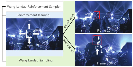
Figure 1. Basis of the proposed Wang–Landau reinforcement sampler. Reinforcement learning proposes one of the action choice (i.e., $a^{left},a^{right},a^{up}$, and $a^{down}$) to move the target state. For example, if $a^{right}$ is selected by our visual tracker, we move the target state to the right. The proposed visual tracker combines this reinforcement learning with Wang–Landau sampling to balance between the exploitation and exploration degrees of the prediction.

1.1. Basic Idea

We further enhance prediction accuracy by balancing the exploitation and exploration abilities of reinforcement learning. The exploitation procedure is used to further simulate the movements at the states around the current local optimum, which the tracker has extensively explored. For example, assume that our visual tracker observes that the target in Figure 1 usually moves to the right, up to the current frame. We likely need to further exploit possible states on the right side of the current state. Our visual tracker can accurately predict the target state using exploitation, especially when the target moves smoothly. In contrast, the exploration procedure is used to simulate the movements at states far from the current local optimum, which the tracker has only minimally explored. For example, the target in Figure 1 moves randomly and inconsistently in some cases; thus, we need to explore unvisited states, far from the current state. Our visual tracker can predict the target state using exploration, especially when the target is fast-moving. Traditional reinforcement learning methods experience difficulty in scheduling the exploitation and exploration procedures. In contrast, our visual tracker overcomes this problem by introducing Wang–Landau sampling [7], in which exploitation and exploration compete against each other in a sampling framework and attain the equivalence status.

1.2. Our Contributions

• We propose a new Q-learning algorithm, augmented by Wang–Landau sampling, in which the exploitation and exploration abilities of reinforcement learning are balanced in searching target states. Conventional Q-learning methods typically select an action that maximizes a current action-value for exploitation, whereas the methods choose an action at random with a probability $ϵ$ for exploration. However, it is nontrivial to determine the optimal $ϵ$, which can balance exploitation and exploration abilities. In contrast, the proposed method can balance between the exploitation and exploration processes based on the Wang–Landau algorithm. The method adapts to control the randomness of policy, using statistics on the number of visits in a particular state. Thus, our method considerably enhances conventional Q-learning algorithm performance, which also enhances visual tracking performance.
• We present a novel visual tracking system based on the Wang–Landau reinforcement sampler. We exhaustively evaluate the proposed visual tracker and numerically demonstrate the effectiveness of the Wang–Landau reinforcement sampler.
• Our visual tracker shows state-of-the-art performance in terms of frames per seconds (FPS) and runs in realtime because our method contains no complicated deep neural network architectures.

The remainder of this paper is organized as follows. In Section 2, we introduce relevant visual tracking algorithms. We explain reinforcement learning-based visual tracking in Section 3.2 and enhance the proposed visual tracking using Wang–Landau sampling in Section 3.3. In Section 4, we evaluate visual tracking algorithms quantitatively and qualitatively. In Section 5, we conclude the paper.

2. Related Work

In this section, we discuss the advantages and disadvantages of the relevant visual tracking methods, which can be categorized into four groups: tracking methods based on reinforcement learning, Wang–Landau sampling, and general visual tracking methods.

2.1. Tracking Methods Based on Reinforcement Learning

For visual tracking, Yun et al. [8] adopted a policy network and defined the actions to localize the target in a current frame. Supancic et al. [9] trained a Q function using the YouTube video dataset and defined the actions used to reinitialize a visual tracker and modify the appearance model of the tracker. However, these trackers could not run in realtime. Thus, Huang et al. [10] enhanced the speed of reinforcement-learning-based visual trackers and maintained their accuracy. They defined actions to determine whether the tracker easily tracks the target. If it is easy, the method tracks the target using inexpensive features; otherwise, the method tracks the target using expensive deep features. Choi et al. [11] ran their tracker at a real-time speed of 43 FPS. They presented lighter-weight deep neural networks and optimized deep neural architectures for matching and policy networks.

In contrast to these methods, our method aims to improve reinforcement learning accuracy by incorporating the Wang–Landau sampling. Please note that Choi et al. [11] did not improve conventional reinforcement learning algorithms but efficiently applied an existing REINFORCE [12] method to target the appearance-updating problem. In contrast, we improve conventional reinforcement learning algorithms (i.e., Q-learning) using Wang–Landau sampling. We enhance conventional Q-learning algorithms to balance the exploitation and exploration abilities of reinforcement learning. Moreover, we adaptively control the randomness of policy using statistics on the number of visits in a particular state.

2.2. Tracking Methods Based on Wang–Landau Sampling

For visual tracking, Kwon and Lee [13] adopted Wang–Landau Monte Carlo (WLMC) sampling to control significant changes in the target’s positions. Zhou et al. [14] enhanced the Wang–Landau samplers and presented a stochastic approximation Monte Carlo (SAMC) sampling-based visual tracker, in which the density of states (DOS) was more accurately estimated with low computational cost. Kwon and Lee [15] extended the WLMC sampling into N-fold Wang–Landau (NFWL) sampling, in which the N-fold algorithm was used to enable the accurate estimation of the DOS with a relatively small number of samples. The NFWL-based visual tracking method can handle significant changes in both the positions and scales of the target. However, these methods do not contain a feedback process and cannot reflect the current visual tracking environment and results. Liu et al. [16] combined WLMC sampling with a visual background extractor, considerably reducing the state space of the target. They independently dealt with scale changes in the target using a fast scale estimation algorithm.

In contrast to these methods, we applied WLMC sampling to reinforcement learning and balanced the exploitation and exploration degrees of the target prediction.

2.3. General Visual Tracking Methods

Because of the representation power of deep neural networks [17,18,19], recent visual trackers have extracted useful features and considerably increased their accuracy [20,21,22,23] referred to as deep learning-based visual tracking methods. Wang et al. [23] presented the first visual tracker that adopted deep features, in which a stacked denoising autoencoder was used to extract generic features, and a classification layer was utilized to determine whether a current image patch is the foreground. Nam et al. [21] considered visual tracking problems as binary classification problems and divided visual tracking videos into multiple domains to extract multidomain features. Ma et al. [20] improved visual tracking accuracy by training deep neural networks using object recognition datasets and extracting hierarchical features. Kwon et al. [24] extracted deep features using the VGG-m network [25] and combined variational autoencoders with the particle Markov chain Monte Carlo method for multiple variable inferences.

Siamese network-based visual trackers [26,27,28] transformed visual tracking problems into matching problems, in which exemplar patches were matched to search window patches through a cross-correlation operation. For this purpose, two deep neural networks were designed with similar architectures that share parameters. Because matching is typically faster than classification, Siamese network-based visual trackers have demonstrated superior speed. Bertinetto et al. [26] implemented a Siamese network using only convolutional layers for visual tracking. Held et al. [28] proposed a Siamese network-based visual tracker that can run at a real-time speed of 100 FPS. Tao et al. [29] introduced a novel approach for visual tracking, in which no model updating was required. They argue that visual tracking accuracy is derived from a powerful matching function, which can be learned using a sufficiently large amount of training data. However, Siamese network-based visual trackers easily miss the targets if there are severe occlusions and background clutter. They lack both an explicit process to obtain feedback from the environment to recover erroneous trajectories and an exploration mechanism to sufficiently search the state space.

To handle long-term video sequences, DASiam [30] considered larger search areas than conventional methods, if target objects have high confidence values. GlobalTrack [31] and SiamRPN [32] have explicit redetection processes, in which whole regions are searched to recover missed target trajectories. However, GlobalTrack and SiamRPN require high computational costs because these methods employ full-search strategies. In contrast, our proposed tracker presents an efficient exploration technique based on Wang–Landau sampling. Thus, our tracker is significantly faster than the aforementioned methods and runs in realtime.

In contrast to the aforementioned methods, we incorporated reinforcement learning into visual tracking problems formulated as action-decision frameworks, in which the proposed method can recover erroneous trajectories using feedback from the environment and sufficiently explore the state space to capture abrupt target motions.

3. Proposed Visual Tracking System

3.1. Bayesian Visual Tracking

The visual tracking system aims to accurately infer target configurations over frames. This inference problem can be formulated using the posterior probability $p\left({\mathbf{X}}_t\right|{\mathbf{Y}}_{1:t})$:

$${\widehat{\mathbf{X}}}_t=\underset{{\mathbf{X}}_t}{arg}maxp\left({\mathbf{X}}_t\right|{\mathbf{Y}}_{1:t}),$$

(1)

where ${\widehat{\mathbf{X}}}_t$ is the best state at time t. We can accurately estimate $p\left({\mathbf{X}}_t\right|{\mathbf{Y}}_{1:t})$ in (1) by adopting Bayesian filtering, which updates the posterior distribution $p\left({\mathbf{X}}_t\right|{\mathbf{Y}}_{1:t})$ using the following rule:

$$\begin{array}{cc}\hfill p\left({\mathbf{X}}_t\right|{\mathbf{Y}}_{1:t})& \propto p\left({\mathbf{Y}}_t\right|{\mathbf{X}}_t)\int p\left({\mathbf{X}}_t\right|{\mathbf{X}}_{t-1})p\left({\mathbf{X}}_{t-1}\right|{\mathbf{Y}}_{1:t-1})d{\mathbf{X}}_{t-1},\hfill \\ \hfill & \approx p\left({\mathbf{Y}}_t\right|{\mathbf{X}}_t)\sum p\left({\mathbf{X}}_t\right|{\mathbf{X}}_{t-1})p\left({\mathbf{X}}_{t-1}\right|{\mathbf{Y}}_{1:t-1}).\hfill \end{array}$$

(2)

where $p\left({\mathbf{Y}}_t\right|{\mathbf{X}}_t)$ denotes the likelihood, i.e., the probability of coincidence between the target object and observation at the proposed state, and $p\left({\mathbf{X}}_t\right|{\mathbf{X}}_{t-1})$ represents the transition kernel that proposes the next state ${\mathbf{X}}_t$ based on the previous state ${\mathbf{X}}_{t-1}$. In (2), $p\left({\mathbf{Y}}_t\right|{\mathbf{X}}_t)$ is defined as

$$p\left({\mathbf{Y}}_t\right|{\mathbf{X}}_t)=e^{-f\left({\mathbf{Y}}_{\mathbf{t}}\left(\mathbf{X}\right),{\mathbf{Y}}^{\mathbf{gt}}\right)},$$

(3)

where f measures the similarity between the observed features [33] of the image described by $\mathbf{X}$, ${\mathbf{Y}}_{\mathbf{t}}\left(\mathbf{X}\right)$ and the ground-truth ${\mathbf{Y}}^{gt}$. We design f, which is similar to the matching function used in [29]. However, it is intractable to integrate probabilities over all possible values of ${\mathbf{X}}_{t-1}$. Alternatively, we can sample a small number of values for ${\mathbf{X}}_{t-1}$ to approximate the integration. If we use an infinite number of samples, the approximation will produce zero errors. However, because it is impractical to use an infinite number of samples in real-world implementations, it is important to determine a limited number of good samples to produce accurate posterior probabilities.

Then, visual tracking aims to accurately approximate posterior probability using mathematical expectation with a limited number of samples [34].

$${\widehat{\mathbf{X}}}_t=\underset{{\mathbf{X}}_t}{arg}max{\mathbb{E}}_{q\left({\mathbf{X}}_t\right|{\mathbf{Y}}_{1:t})}\left[logp\left({\mathbf{X}}_t\right|{\mathbf{Y}}_{1:t})\right],$$

(4)

where $q\left({\mathbf{X}}_t\right|{\mathbf{Y}}_{1:t})$ is the function that outputs ${\mathbf{X}}_t$ given ${\mathbf{Y}}_{1:t}$. In (4), $q\left({\mathbf{X}}_t\right|{\mathbf{Y}}_{1:t})$ is designed by selecting the optimal transition kernel $p^{*}\left({\mathbf{X}}_t\right|{\mathbf{X}}_{t-1})$, as follows:

$$q\left({\mathbf{X}}_t\right|{\mathbf{Y}}_{1:t})=p\left({\mathbf{Y}}_t\right|{\mathbf{X}}_t)\sum p^{*}\left({\mathbf{X}}_t\right|{\mathbf{X}}_{t-1})p\left({\mathbf{X}}_{t-1}\right|{\mathbf{Y}}_{1:t-1}).$$

(5)

3.2. Reinforcement Learning for Visual Tracking

In this study, $p^{*}\left({\mathbf{X}}_t\right|{\mathbf{X}}_{t-1})$ in (5) is implemented by selecting the optimal action $a_t$ in a reinforcement learning framework, in which ${\mathbf{X}}_{t+1}\sim a_t(·|{\mathbf{X}}_t)$. We compute the reward $\mathcal{R}$ by measuring the improvement in the log-posterior probability in (2), as follows:

$$\mathcal{R}(s_t,a_t,s_{t+1})=logp\left({\mathbf{X}}_t\right|{\mathbf{Y}}_{1:t})-logp\left({\mathbf{X}}_{t+1}\right|{\mathbf{Y}}_{1:t+1}),$$

(6)

where $s_t=\left\{{\mathbf{X}}_{1:t}\right\}$. In (6), $s_t,s_{t+1}\in \mathcal{S}$ and $a_t\in \mathcal{A}$, where $\mathcal{S}$ and $\mathcal{A}$ denote the spaces of states and actions, respectively. $\mathcal{A}$ can have four possible actions, $\{a^{left},a^{right},a^{up},a^{down}\}$:

$$\mathcal{A}=\left\{\begin{array}{c}{a}^{left}:p_x\to p_x-1,p_y\to p_y,\hfill \\ a^{right}:p_x\to p_x+1,p_y\to p_y,\hfill \\ a^{up}:p_y\to p_y-1,p_x\to p_x,\hfill \\ a^{down}:p_y\to p_y+1,p_x\to p_x,\hfill \end{array}\right.$$

(7)

where $p_x$ and $p_y$ are the pixel indexes at the x and y axes, respectively.

Our visual tracker aims to find the optimal policy ${\pi }^{*}:\mathcal{S}\to \mathcal{A}$ that maximizes the expected future reward at time t:

$${\pi }^{*}=\underset{\pi }{arg}max{\mathbb{E}}_{\pi }\left[{\mathcal{R}}_{t+1}+\gamma {\mathcal{R}}_{t+2}+{\gamma }^2{\mathcal{R}}_{t+3}+\cdots +{\gamma }^{\tau -t-1}{\mathcal{R}}_{\tau }\right],$$

(8)

for a single episode of length $\tau$, where $\gamma <1$ is a discounting parameter that weights rewards that can be received immediately. The expected cumulative reward in (8) is efficiently implemented by Q-learning [35] with the following updating rule:

$$Q(s_t,a_t)\leftarrow Q(s_t,a_t)+\alpha \left[{\mathcal{R}}_{t+1}+\gamma \underset{a}{max}Q(s_{t+1},a)-Q(s_t,a_t)\right],$$

(9)

where $\gamma \underset{a}{max}Q(s_{t+1},a)-Q(s_t,a_t)$ indicates the maximum update of the action-value function $Q(s_t,a_t)$ at time t. This update is caused by a state change from $s_t$ to $s_{t+1}$ through action a. In (9), ${\mathcal{R}}_{t+1}$ is the reward at time $t+1$ and $\alpha$ is a weighting parameter.

The optimal policy in (8) can be determined toward maximizing the Q-values:

$${\pi }^{*}(·|s)=\underset{a}{arg}maxQ(s,a),$$

(10)

where the next action $a_{t+1}$ is sampled by ${\pi }^{*}\left(a_t\right|s_t)$ and the next state $s_{t+1}$ is determined by (7). However, when using (10), there is a risk of choosing suboptimal actions because we select an action that maximizes only a current action value. This problem causes our visual tracker to explore only already-visited states, which become trapped in the local optimum.

We overcome this problem by proposing the $ϵ$-$greedy$ algorithm, in which we usually select an action that maximizes a current action-value; with a probability $ϵ$, we choose an action at random. This $ϵ$-$greedy$ algorithm can be expressed as

$$a\sim \left\{\begin{array}{cc}\underset{a}{arg}maxQ(s,a),\hfill & \mathrm{with}\mathrm{probability}1-ϵ\hfill \\ random\left(\mathcal{A}\right)\hfill & \mathrm{with}\mathrm{probability}ϵ,\hfill \end{array}\right.$$

(11)

where $random\left(\mathcal{A}\right)$ returns an action randomly. However, one of the difficulties we may experience when using $ϵ$-$greedy$, as a result of randomness in (11), is the surplus of actions, which complicates optimal solution identification. Therefore, we propose a semirandom strategy based on the Wang–Landau algorithm [7], in which we control the randomness of policy using statistics on the number of visits in a particular state. This approach will be further explained in the following section.

3.3. Wang–Landau Reinforcement Sampler for Visual Tracking

The proposed Wang–Landau sampler can be used to encourage the exploration of reinforcement learning by estimating the DOS [15], in which the DOS value approximates the frequency of visits to each state using Monte Carlo simulations. Based on the DOS, we determine whether a particular state is sufficiently explored. If a state has a small DOS value, the Wang–Landau sampler guides the reinforcement learning to explore that state. Otherwise, the sampler refrains from exploring that state.

For Wang–Landau sampling, we define $\mathbf{D}={\left\{d_i\right\}}_{i=1}^{\left|\mathcal{S}\right|}$ and $\mathbf{V}={\left\{v_i\right\}}_{i=1}^{\left|\mathcal{S}\right|}$, in which $d_i$ and $v_i$ are the DOS score and the number of visits for the i-th state, respectively, and $\left|\mathcal{S}\right|$ is the total number of states. Then, we update $d_i$ if the visual tracker visits the i-th state:

$$d_i\leftarrow d_i\times w,\forall i,$$

(12)

where $w>1$ is a weighting parameter. $v_i$ is updated as follows:

$$v_i\leftarrow v_i+1,\forall i,$$

(13)

where $d_i$ and $v_i$ are initialized to 1 and 0, respectively. As the iteration proceeds, the Wang–Landau sampling adopts a coarse-to-fine strategy to attain more accurate DOS values. In the early iteration, we use a large value of w in (12), which increases the update speed. In the latter iteration, we use a smaller value of wm to fine-tune the updates. Accordingly, we decrease the value of w, $w\leftarrow \sqrt{w}$, if a current iteration satisfies the following condition, i.e., the semiflat status:

$$\forall i,v_i\ge 0.8\times \frac{1}{\left|\mathcal{S}\right|}\sum _{\forall i}{v}_i,$$

(14)

where we, at least partially, explore all states. After the modification of w, the value $v_i$ is reinitialized to 0.

Owing to the need to balance the exploration of reinforcement learning with its exploitation, we present a new scheduling approach for reinforcement learning, as follows:

$$a\sim \left\{\begin{array}{cc}\underset{a}{arg}maxQ(s,a),\hfill & \mathrm{with}\mathrm{probability}1-{ϵ}^{new}\hfill \\ random\left(\mathcal{A}\right)\hfill & \mathrm{with}\mathrm{probability}{ϵ}^{new},\hfill \end{array}\right.$$

(15)

with

$${ϵ}^{new}=max\left[1,\frac{d_i}{p_i\left({\mathbf{Y}}_t\right|{\mathbf{X}}_t)}\right],$$

(16)

where $p_i\left({\mathbf{Y}}_t\right|{\mathbf{X}}_t)$ is the likelihood at the i-th state, which is defined in (3). In (16), exploration $d_i$ and exploitation $p_i\left({\mathbf{Y}}_t\right|{\mathbf{X}}_t)$ compete with each other. For example, if $d_i$ increases with respect to $p_i\left({\mathbf{Y}}_t\right|{\mathbf{X}}_t)$, reinforcement learning would explore diverse states with a high probability. If not, it tends to exploit a current state with a high probability.

Algorithm 1 illustrates the complete process of the proposed method.

Algorithm 1 Wang–Landau reinforcement sampler

1: Input:${\widehat{\mathbf{X}}}_t$, $d_i=1$, $v_i=0$, $\forall i$, and $w>1$.    2: Output:${\widehat{\mathbf{X}}}_{t+1}$  3: for$j=1$ to N do  4:   • Reinforcement learning    5:   Propose an action a according to (15).    6:   Find the next state ${\mathbf{X}}_{t+1}$ using the proposed action in (7).  7:   Computer the posterior probability $p\left({\mathbf{X}}_{t+1}\right|{\mathbf{Y}}_{1:t})$ in (2).  8:   Estimate the reward ${\mathcal{R}}_{t+1}$ using $p\left({\mathbf{X}}_{t+1}\right|{\mathbf{Y}}_{1:t})$ in (6).  9:   Update the Q value using ${\mathcal{R}}_{t+1}$ in (9). 10:  Determine the optimal policy function $\pi$ using Q in (10). 11:  • Wang–Landau Monte Carlo sampling 12:  Find the index i of the state ${\mathbf{X}}_{t+1}$.   13:  Update the DOS score $d_i$ using (12).   14:  Update the number of visits $v_i$ using (13).   15:  if $v_i$ reaches the semiflat status in (14) then 16:   $w\leftarrow \sqrt{w}$.   17:   $v_i=0$.   18:  end if  19: end for  20: Find the best configuration ${\widehat{\mathbf{X}}}_{t+1}$ using (1).

4. Experiments

4.1. Experimental Settings

The proposed method was compared with 30 non-deep learning methods (e.g., SCM [36], STRUCK [37], ASLA [38], TLD [39], CXT [40], VTD [41], VTS [42], CSK [43], MEEM [44], Staple [45], and SRDCF [46]) on 50 test sequences in the OTB dataset [47]. Furthermore, our method was compared to state-of-the-art deep learning-based methods: C-COT [48], SINT [29], SINT-op [29], ECO [49], ECO-HC [49], SiamRPN++ [32], TADT [50], DAT [51], and SiamDW [52]. Moreover, the proposed visual tracker was compared based on the VOT2017 [53] dataset with 10 recent visual trackers, including CFWCR [54], CFCF [55], CSRDCF [56], MCCT [57], and LSART [58]. Our proposed visual tracker was also compared for the LaSOT [59] dataset with 8 state-of-the-art visual trackers, namely ECO [49], SiamRPN++ [32], GlobalTrack [31], ATOM [60], DASiam [30], CFNet [61], SPLT [62], and StructSiam [63]. Please note that we compared the proposed method with 30 non-deep learning visual trackers but reported only top 10 visual tracker in Figure 2 to visualize precision and success curves for each tracker more clearly.

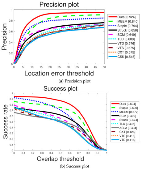
Figure 2. Quantitative comparison with non-deep learning based methods. We evaluate the methods using precision and success plots in (a,b), respectively.

We used the precision, success rate, and AUC as evaluation metrics for testing these methods [47]. For precision, we calculated the $l2$-norm distance between the estimated bounding box $E_t$ and the ground truth bounding box $G_t$. Then, we depicted the precision plot, which shows the percentage of frames such that the $l2$-norm distance is less than a specific threshold. For the success rate, we calculated the intersection of union $IoU=\frac{|E_t\cap G_t|}{|E_t\cup G_t|}$, where $|·|$ indicates the number of pixels. We considered visual tracking at each frame to be successful, if $IoU$ is greater than a specific threshold. Moreover, we calculated the success rate, which is the ratio of the number of successful frames to the number of total frames. We then illustrated the success plot, which presents the success rates with different thresholds, and we calculated the area under curve (AUC).

For fair comparison, we used the best visual tracking results reported by the authors in the original papers and followed their experimental settings. For example, SiamRPN++ [32] was pretrained on ImageNet [64] and used ResNet [33] as a backbone network. In addition, SiamRPN++ was trained using the training datasets of COCO [65], ImageNet DET [64], ImageNet VID, and the YouTube-Bounding Boxes dataset [66]. All experiments were conducted using a desktop with an Intel CPU i7 3.60 GHz and GeForce Titan XP graphics card for the proposed method. Throughout the experiments, hyperparameters were fixed as follows: $\gamma =0.9$ in (8), $N=2000$ in Algorithm 1 and $w=0.8$ in (12).

4.2. Ablation Study

We examined the effectiveness of the Wang–Landau sampling for reinforcement learning and sensitivity to hyperparameters of our method. Table 1 compares two variants of our method: reinforcement learning-based visual trackers with $ϵ$-greedy and Wang–Landau sampling. Table 1 demonstrates that the accuracy of reinforcement learning-based visual trackers can be considerably increased if the exploration and exploitation abilities are balanced by Wang–Landau sampling. Table 2 shows the visual tracking results of our method using different values of hyperparameters. If $\gamma$ in (8) increases, our method imposes more weights on rewards in the near future. If $N=2000$ in Algorithm 1 has a larger value, our method can more accurately estimate the DOS score and Q-values, sacrificing computational cost. If $w=0.8$ in (12) is larger, our method can estimate the DOS score with a smaller number of iterations but less accurately. As shown in Table 2, our method is insensitive to hyperparameters. Although the values of these hyperparameters severely change, our method consistently produces accurate visual tracking results, because our proposed Q-learning-based reinforcement method accurately predicts target states regardless of the hyperparameter values.

Table 1. Ablation study: Effectiveness of Wang–Landau sampling for reinforcement learning-based visual tracking.

	$\mathit{ϵ}$-Greedy	Wang–Landau Sampling
AUC	0.583	0.694

Table 2. Ablation study: Sensitivity to hyperparameters, $\gamma$ in (8), N in Algorithm 1, and w in (12).

$\mathit{\gamma }$	0.8	0.9	1.0
AUC	0.651	0.694	0.647
$\mathit{N}$	1000	2000	3000
AUC	0.642	0.694	0.649
$\mathit{w}$	0.7	0.8	0.9
AUC	0.650	0.694	0.637

4.3. Quantitative Comparison

Figure 2 shows the quantitative comparisons with non-deep learning-based visual trackers. Our method considerably outperformed the second-best trackers, MEEM and Staple, in terms of precision and success rate, respectively. Our method was able to accurately track the target despite the severe appearance of the target. In particular, the proposed Wang–Landau Monte Carlo sampling improves the exploration of unvisited states, enabling our tracker to cover abrupt motion changes of the target.

Figure 3 shows the quantitative comparisons with recent deep-learning-based visual trackers. SiamDW was the best in terms of the precision plot, and ECO was the best in terms of the success plot. As shown in Figure 3, our method was competitive with deep learning-based visual trackers. In particular, our method produced accurate tracking results in terms of the success plot but relatively inaccurate tracking results in terms of the precision plot, implying that our method can be improved by adopting multiscale approaches.

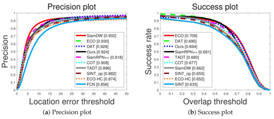
Figure 3. Quantitative comparison with deep learning based methods in terms of precision and success rate.

In Figure 4, we highlighted experiments on test sequences, which contain examples of interrupted and recovered tracking. For example, “Out of view” and “Occlusion” sequences contain interrupted and recovered tracking scenarios. In these sequences, target objects frequently disappear due to occlusion and out of view attributes, which causes conventional trackers to miss the target trajectories. After a long time, the targets reappear and the trackers need to recover the target trajectories. In this situation, the proposed tracker efficiently recovers missing trajectories using the proposed exploration mechanism. As shown in Figure 4, the propose visual tracker considerably outperforms other state-of-the-art deep-learning visual trackers, which demonstrates the effectiveness of the proposed exploration mechanism based on Wang–Landau sampling.

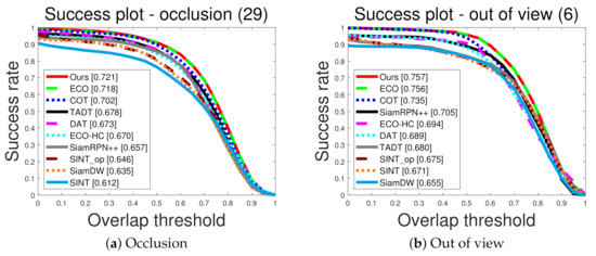
Figure 4. Quantitative comparison in term of the success plot for interrupted and recovered tracking scenarios.

Figure 5 quantitatively evaluates the proposed method (ours) and the recent state-of-the-art deep-learning-based visual trackers using the VOT2014 dataset. Our method considerably outperforms other methods in terms of accuracy. Staple shows the second-best accuracy. However, robustness is significantly worse than the proposed method, implying that our method rarely missed the targets, while preserving the accuracy over frames. Gnet is the best in terms of robustness, while its accuracy is lower than ours.

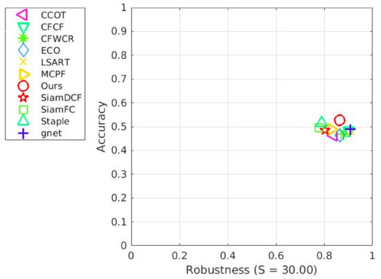
Figure 5. Quantitative comparison of our method with recent state-of-the-art deep-learning visual trackers using the VOT2017 dataset.

Table 3 quantitatively evaluates the proposed method and deep-learning-based visual tracking methods using the LaSOT dataset. Our method and GlobalTrack present state-of-the-art tracking performance. GlobalTrack has an explicit redetection, which requires accurate object detectors. In contrast, the efficient performance of the proposed method stems from reinforcement learning with Wang–Landau-based exploration. Our method implicitly searches for the targets without any object detector.

Table 3. Quantitative comparison of our method with recent deep-learning-based visual tracking methods using the LaSOT dataset.

	GlobalTrack	ATOM	SiamRPN++	DASiam	SPLT	StructSiam	CFNet	ECO	Ours
AUC	0.521	0.518	0.496	0.448	0.426	0.335	0.275	0.324	0.519
Precision	0.529	0.506	0.491	0.427	0.396	0.333	0.259	0.301	0.541
Normalized	0.599	0.576	0.569	-	0.494	0.418	0.312	0.338	0.605

Table 4 quantitatively evaluates the computational costs of recent visual trackers using the LaSOT dataset. Our visual tracker shows state-of-the-art performance in terms of FPS and can run in realtime because our method contains no complicated deep neural network architectures.

Table 4. Computational costs of visual trackers in terms of frames per seconds (FPS).

	GlobalTrack	ATOM	SiamRPN++	DASiam	SPLT	StructSiam	CFNet	ECO	Ours
FPS	6	30	35	110	26	45	15	5	115

Figure 6 measured the recovery rated for 8 state-of-the-art visual trackers, namely ECO, SiamRPN++, GlobalTrack, ATOM, DASiam, CFNet, SPLT, and StructSiam using the LaSOT dataset. We counted the average number of frames such that $IoU$ is zero (i.e., the average number of interruptions), which means that trackers missed the targets. After each frame such that $IoU=0$, we counted the average number of frames such that $IoU$ becomes nonzero again (i.e., the average number of recovered trajectories), which means that trackers recovered the targets. The recovery rate was calculated by dividing the average number of recovered trajectories with the average number of interruptions. As shown in Figure 6, our method considerably surpasses other methods in terms of the recovery rate, which demonstrate the effectiveness of the proposed Wang–Landau reinforcement sampler.

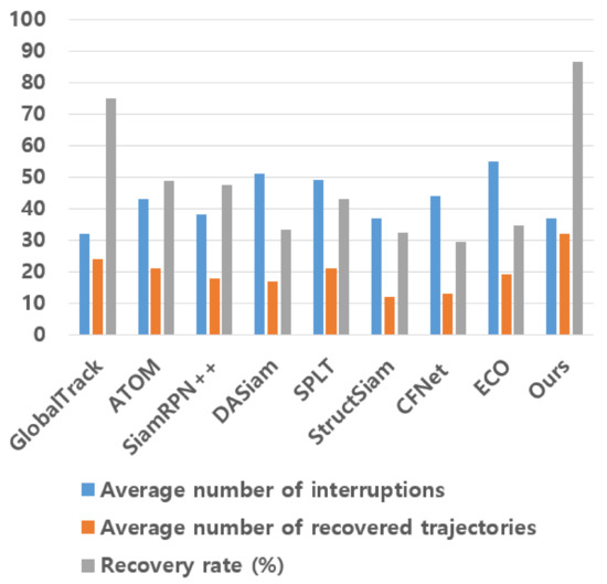
Figure 6. Comparison on the recovery rate. Blue, orange, and gray bars denote the average number of interruptions, the average number of recovered trajectories, and recovery rate (i.e., $\frac{\mathrm{average}\mathrm{number}\mathrm{of}\mathrm{recovered}\mathrm{trajectories}}{\mathrm{average}\mathrm{number}\mathrm{of}\mathrm{interruptions}}\times 100$), respectively.

4.4. Qualitative Comparison

Figure 7 qualitatively compares our method with the method based on conventional $ϵ$-$greedy$ reinforcement learning using the OTB dataset. Although the test sequences contained abrupt motions (e.g., Deer, Shaking, MotorRolling, and Biker sequences), severe deformation (e.g., Ironman, Diving, Jump, Skiing, and Surfer sequences), occlusion (Soccer sequence), and illumination changes (e.g., Matrix, Shaking, and Skating1 sequences), our method accurately tracked the targets. However, conventional reinforcement learning with $ϵ$-$greedy$ frequently failed to track the targets when there were abrupt motions occurred because it could not sufficiently explore unvisited states.

Figure 7. Qualitative comparisons. White boxes present the estimated bounding boxes of our method, while red boxes represent the results of our method without Wang–Landau sampling.

Figure 8 shows qualitative visual tracking results of the proposed method with and without the Wang–Landau algorithm using the LaSOT dataset. The video sequences include tiny objects (e.g., boat-12, crocodile-3, drone-13, elephant-18, fox-3, and flog-9 sequences), background clutter (e.g., chameleon-6, cram-18, and fox-3 sequences), nonrigid objects (e.g., bear-17, bird-17, cattle-7, crocodile-3, fox-3, frog-9, and giraffe-10 sequences), motion blur (e.g., bus-5 and crab-18 sequences), and rotation (e.g., bottle-1 sequence). Despite these challenging visual tracking environments, the proposed method accurately tracked the targets. These results indicate that the proposed Wang–Landau-based reinforcement learning is helpful for finding unexplored states and recovering missed trajectories. As shown in Figure 8, the proposed Wang–Landau algorithm helps our visual tracker to recover inaccurate bounding boxes.

Figure 8. Qualitative evaluation. White and green boxes present the predicted bounding boxes of the proposed method with and without the Wang–Landau algorithm.

In summary, the proposed method works better than other state-of-the-art methods, as follows. Our method can predict the target state with greater accuracy by defining multiple actions in a reinforcement learning framework and moving the current state according to the selected action. In addition, we further enhance prediction accuracy by improving reinforcement learning performance using Wang–Landau sampling, in which exploitation and exploration compete against each other in a sampling framework and attain the equivalence status.

5. Conclusions

In this study, we present a visual tracking system based on reinforcement learning, in which the accuracy of the tracking can be considerably enhanced by target configuration prediction for the subsequent frame. Our visual tracker is improved by Wang–Landau sampling, in which the exploration and exploitation of reinforcement learning are efficiently scheduled. The experimental results demonstrate that our method significantly outperforms non-deep learning-based visual tracking methods. Our method is competitive with deep learning-based visual trackers, whereas the proposed method is the fastest algorithm among the compared visual trackers. For future work, we adopt the deep Q learning method to improve the visual tracking accuracy, which is one of the well-known deep learning-based reinforcement learning approaches.

Our method can fail to track the targets, if the target motions are highly random. In this case, the proposed re-reinforcement learning method inaccurately predicts the target position and degrades visual tracking performance. For future research, we plan to integrate explicit object detector into the proposed framework to handle random motions.

References

- Sui, Y.; Zhang, L. Visual Tracking via Locally Structured Gaussian Process Regression. IEEE SPL 2015, 22, 1331–1335. [Google Scholar] [CrossRef]
- Wang, L.; Lu, H.; Wang, D. Visual Tracking via Structure Constrained Grouping. IEEE SPL 2014, 22, 794–798. [Google Scholar] [CrossRef]
- Xu, Y.; Ni, B.; Yang, X. When Correlation Filters Meet Convolutional Neural Networks for Visual Tracking. IEEE SPL 2016, 23, 1454–1458. [Google Scholar]
- Kwon, J.; Dragon, R.; Gool, L.V. Joint Tracking and Ground Plane Estimation. IEEE SPL 2016, 23, 1514–1517. [Google Scholar] [CrossRef]
- Kim, H.; Jeon, S.; Lee, S.; Paik, J. Robust Visual Tracking Using Structure-Preserving Sparse Learning. IEEE SPL 2017, 24, 707–711. [Google Scholar] [CrossRef]
- Xu, Y.; Wang, J.; Li, H.; Li, Y.; Miao, Z.; Zhang, Y. Patch-based Scale Calculation for Real-time Visual Tracking. IEEE SPL 2016, 23, 40–44. [Google Scholar]
- Wang, F.; Landau, D. Efficient, multiple-range random walk algorithm to calculate the density of states. Phys. Rev. Lett. 2001, 86, 2050–20531. [Google Scholar] [CrossRef]
- Yun, S.; Choi, J.; Yoo, Y.; Yun, K.; Choi, J.Y. Action-Decision Networks for Visual Tracking with Deep Reinforcement Learning. In Proceedings of the IEEE Conference on Computer Vision and Pattern Recognition, Honolulu, HI, USA, 21–26 July 2017. [Google Scholar]
- Supancic, J., III; Ramanan, D. Tracking as Online Decision-Making: Learning a Policy From Streaming Videos with Reinforcement Learning. In Proceedings of the IEEE International Conference on Computer Vision ICCV, Venice, Italy, 22–29 October 2017. [Google Scholar]
- Huang, C.; Lucey, S.; Ramanan, D. Learning Policies for Adaptive Tracking with Deep Feature Cascades. In Proceedings of the IEEE International Conference on Computer Vision ICCV, Venice, Italy, 22–29 October 2017. [Google Scholar]
- Choi, J.; Kwon, J.; Lee, K.M. Real-time Visual Tracking by Deep Reinforced Decision Making. Comput. Vis. Image Underst. 2018, 171, 10–19. [Google Scholar] [CrossRef]
- Williams, R.J. Simple statistical gradient-following algorithms for connectionist reinforcement learning. Mach. Learn. 1992, 8, 229–256. [Google Scholar] [CrossRef]
- Kwon, J.; Lee, K.M. Tracking of Abrupt Motion using Wang-Landau Monte Carlo Estimation. In Proceedings of the 10th European Conference on Computer Vision, Marseille, France, 12–18 October 2008. [Google Scholar]
- Zhou, X.; Lu, Y. Abrupt Motion Tracking via Adaptive Stochastic. Approximation Monte Carlo Sampling. In Proceedings of the 2010 IEEE Computer Society Conference on Computer Vision and Pattern Recognition, San Francisco, CA, USA, 13–18 June 2010. [Google Scholar]
- Kwon, J.; Lee, K.M. Wang-Landau Monte Carlo-based Tracking Methods for Abrupt Motions. IEEE Trans. Pattern Anal. Mach. Intell. 2013, 35, 1011–1024. [Google Scholar] [CrossRef]
- Liu, J.; Zhou, L.; Zhao, L. Advanced wang-landau monte carlo-based tracker for abrupt motions. IEEJ Trans. Electr. Electron. Eng. 2019, 14, 877–883. [Google Scholar] [CrossRef]
- LeCun, Y.; Bottou, L.; Bengio, Y.; Haffner, P. Gradient-based learning applied to document recognition. Proc. IEEE 1998, 86, 2278–2324. [Google Scholar] [CrossRef]
- Krizhevsky, A.; Sutskever, I.; Hinton, G.E. Imagenet classification with deep convolutional neural networks. Commun. ACM 2017, 60, 84–90. [Google Scholar] [CrossRef]
- Ren, S.; He, K.; Girshick, R.; Sun, J. Faster R-CNN: Towards real-time object detection with region proposal networks. IEEE Trans. Pattern Anal. Mach. Intell. 2016, 39, 1137–1149. [Google Scholar] [CrossRef] [PubMed]
- Ma, C.; Huang, J.B.; Yang, X.; Yang, M.H. Hierarchical Convolutional Features for Visual Tracking. In Proceedings of the IEEE International Conference on Computer Vision, Santiago, Chile, 7–13 December 2015. [Google Scholar]
- Nam, H.; Han, B. Learning Multi-Domain Convolutional Neural Networks for Visual Tracking. In Proceedings of the IEEE Conference on Computer Vision and Pattern Recognition, Las Vegas, NV, USA, 27–30 June 2016. [Google Scholar]
- Wang, L.; Ouyang, W.; Wang, X.; Lu, H. Stct: Sequentially training convolutional networks for visual tracking. In Proceedings of the IEEE Conference on Computer Vision and Pattern Recognition, Las Vegas, NV, USA, 27–30 June 2016. [Google Scholar]
- Wang, N.; Yeung, D.Y. Learning a deep compact image representation for visual tracking. In Advances in Neural Information Processing Systems; The MIT Press: Cambridge, MA, USA, 2013. [Google Scholar]
- Kwon, J. Robust Visual Tracking based on Variational Auto-encoding Markov Chain Monte Carlo. Inf. Sci. 2020, 512, 1308–1323. [Google Scholar] [CrossRef]
- Chatfield, K.; Simonyan, K.; Vedaldi, A.; Zisserman, A. Return of the devil in the details: Delving deep into convolutional nets. arXiv 2014, arXiv:1405.3531. [Google Scholar]
- Bertinetto, L.; Valmadre, J.; Henriques, J.F.; Vedaldi, A.; Torr, P.H. Fully-Convolutional Siamese Networks for Object Tracking. arXiv 2016, arXiv:1606.09549. [Google Scholar]
- Chen, K.; Tao, W. Once for All: A Two-flow Convolutional Neural Network for Visual Tracking. arXiv 2016, arXiv:1604.07507. [Google Scholar] [CrossRef]
- Held, D.; Thrun, S.; Savarese, S. Learning to Track at 100 FPS with Deep Regression Networks. In Proceedings of the European Conference on Computer Vision, Amsterdam, The Netherlands, 8–16 October 2016. [Google Scholar]
- Tao, R.; Gavves, E.; Smeulders, A.W. Siamese Instance Search for Tracking. In Proceedings of the IEEE Conference on Computer Vision and Pattern Recognition, Las Vegas, NV, USA, 27–30 June 2016. [Google Scholar]
- Zhu, Z.; Wang, Q.; Li, B.; Wu, W.; Yan, J.; Hu, W. Distractor-Aware Siamese Networks for Visual Object Tracking. In Proceedings of the European Conference on Computer Vision, Munich, Germany, 8–14 September 2018. [Google Scholar]
- Huang, L.; Zhao, X.; Huang, K. GlobalTrack: A Simple and Strong Baseline for Long-term Tracking. arXiv 2019, arXiv:1912.08531. [Google Scholar]
- Li, B.; Wu, W.; Wang, Q.; Zhang, F.; Xing, J.; Yan, J. SiamRPN++: Evolution of Siamese Visual Tracking with Very Deep Networks. In Proceedings of the IEEE Conference on Computer Vision and Pattern Recognition, Long Beach, CA, USA, 15–20 June 2019. [Google Scholar]
- He, K.; Zhang, X.; Ren, S.; Sun, J. Deep residual learning for image recognition. In Proceedings of the IEEE Conference on Computer Vision and Pattern Recognition, Las Vegas, NV, USA, 27–30 June 2016. [Google Scholar]
- Shi, T.; Steinhardt, J.; Liang, P. Learning Where to Sample in Structured Prediction. In Artificial Intelligence and Statistics; The MIT Press: Cambridge, MA, USA, 2015. [Google Scholar]
- Watkins, C.; Dayan, P. Q-learning, in Machine learning. Mach. Learn. 1992, 8, 279–292. [Google Scholar] [CrossRef]
- Zhong, W.; Lu, H.; Yang, M.H. Robust Object Tracking via Sparsity-based Collaborative Model. In Proceedings of the 2012 IEEE Conference on Computer Vision and Pattern Recognition, Providence, RI, USA, 16–21 June 2012. [Google Scholar]
- Hare, S.; Saffari, A.; Torr, P.H.S. Struck: Structured Output Tracking with Kernels. In Proceedings of the 2011 International Conference on Computer Vision, Barcelona, Spain, 6–13 November 2011. [Google Scholar]
- Jia, X.; Lu, H.; Yang, M.H. Visual Tracking via Adaptive Structural Local Sparse Appearance Model. In Proceedings of the 2012 IEEE Conference on Computer Vision and Pattern Recognition, Providence, RI, USA, 16–21 June 2012. [Google Scholar]
- Kalal, Z.; Mikolajczyk, K.; Matas, J. Tracking-Learning-Detection. IEEE Trans. Pattern Anal. Mach. Intell. 2012, 34, 1409–1422. [Google Scholar] [CrossRef]
- Dinh, T.B.; Vo, N.; Medioni, G. Context Tracker: Exploring Supporters and Distracters in Unconstrained Environments. In Proceedings of the IEEE Conference on Computer Vision and Pattern Recognition, Providence, RI, USA, 20–25 June 2011. [Google Scholar]
- Kwon, J.; Lee, K.M. Visual Tracking Decomposition. In Proceedings of the IEEE Conference on Computer Vision and Pattern Recognition, San Francisco, CA, USA, 13–18 June 2010. [Google Scholar]
- Kwon, J.; Lee, K.M. Tracking by Sampling Trackers. In Proceedings of the International Conference on Computer Vision, Barcelona, Spain, 6–13 November 2011. [Google Scholar]
- Henriques, J.; Caseiro, R.; Martins, P.; Batista, J. Exploiting the circulant structure of tracking-by-detection with kernels. In European Conference on Computer Vision; Springer: Berlin/Heidelberg, Germany, 2012. [Google Scholar]
- Zhang, J.; Ma, S.; Sclaroff, S. MEEM: Robust tracking via multiple experts using entropy minimization. In European Conference on Computer Vision; Springer: Cham, Switzerland, 2014. [Google Scholar]
- Bertinetto, L.; Valmadre, J.; Golodetz, S.; Miksik, O.; Torr, P. Staple: Complementary Learners for Real-Time Tracking. In Proceedings of the IEEE Conference on Computer Vision and Pattern Recognition, Las Vegas, NV, USA, 27–30 June 2016. [Google Scholar]
- Danelljan, M.; Häger, G.; Khan, F.; Felsberg, M. Learning Spatially Regularized Correlation Filters for Visual Tracking. In Proceedings of the IEEE International Conference on Computer Vision, Santiago, Chile, 7–13 December 2015. [Google Scholar]
- Wu, Y.; Lim, J.; Yang, M.H. Online object tracking: A benchmark. In Proceedings of the IEEE Conference on Computer Vision and Pattern Recognition, Portland, Oregon, 23–28 June 2013. [Google Scholar]
- Danelljan, M.; Robinson, A.; Khan, F.; Felsberg, M. Beyond Correlation Filters: Learning Continuous Convolution Operators for Visual Tracking. In European Conference on Computer Vision; Springer: Cham, Switzerland, 2016. [Google Scholar]
- Danelljan, M.; Bhat, G.; Shahbaz Khan, F.; Felsberg, M. ECO: Efficient Convolution Operators for Tracking. In Proceedings of the IEEE Conference on Computer Vision and Pattern Recognition, Honolulu, HI, USA, 21–26 July 2017. [Google Scholar]
- Li, X.; Ma, C.; Wu, B.; He, Z.; Yang, M.H. Target-Aware Deep Tracking. In Proceedings of the IEEE Conference on Computer Vision and Pattern Recognition, Long Beach, CA, USA, 15–20 June 2019. [Google Scholar]
- Pu, S.; Song, Y.; Ma, C.; Zhang, H.; Yang, M.H. Deep Attentive Tracking via Reciprocative Learning. In Advances in Neural Information Processing Systems; The MIT Press: Cambridge, MA, USA, 2018. [Google Scholar]
- Zhang, Z.; Peng, H. Deeper and Wider Siamese Networks for Real-Time Visual Tracking. In Proceedings of the IEEE Conference on Computer Vision and Pattern Recognition, Long Beach, CA, USA, 15–20 June 2019. [Google Scholar]
- Kristan, M.; Leonardis, A.; Matas, J.; Felsberg, M.; Pflugfelder, R.; Čehovin Zajc, L.; Vojir, T.; Häger, G.; Lukežič, A.; Eldesokey, A.; et al. The Visual Object Tracking VOT2017 Challenge Results. In Proceedings of the IEEE International Conference on Computer Vision Workshops, Venice, Italy, 22–29 October 2017. [Google Scholar]
- He, Z.; Fan, Y.; Zhuang, J.; Dong, Y.; Bai, H. Correlation Filters with Weighted Convolution Responses. In Proceedings of the IEEE International Conference on Computer Vision Workshops, Venice, Italy, 22–29 October 2017. [Google Scholar]
- Gundogdu, E.; Alatan, A.A. Good Features to Correlate for Visual Tracking. arXiv 2017, arXiv:1704.06326. [Google Scholar] [CrossRef]
- Lukezic, A.; Vojir, T.; Zajc, L.C.; Matas, J.; Kristan, M. Discriminative Correlation Filter with Channel and Spatial Reliability. In Proceedings of the IEEE Conference on Computer Vision and Pattern Recognition, Honolulu, HI, USA, 21–26 July 2017. [Google Scholar]
- Wang, N.; Zhou, W.; Tian, Q.; Hong, R.; Wang, M.; Li, H. Multi-Cue Correlation Filters for Robust Visual Tracking. In Proceedings of the IEEE Conference on Computer Vision and Pattern Recognition, Salt Lake City, UT, USA, 18–23 June 2018. [Google Scholar]
- Sun, C.; Wang, D.; Lu, H.; Yang, M.H. Learning Spatial-Aware Regressions for Visual Tracking. In Proceedings of the IEEE Conference on Computer Vision and Pattern Recognition, Salt Lake City, UT, USA, 18–23 June 2018. [Google Scholar]
- Fan, H.; Lin, L.; Yang, F.; Chu, P.; Deng, G.; Yu, S.; Bai, H.; Xu, Y.; Liao, C.; Ling, H. LaSOT: A High-quality Benchmark for Large-scale Single Object Tracking. arXiv 2018, arXiv:1809.07845. [Google Scholar]
- Danelljan, M.; Bhat, G.; Khan, F.S.; Felsberg, M. Atom: Accurate tracking by overlap maximization. In Proceedings of the IEEE Conference on Computer Vision and Pattern Recognition, Long Beach, CA, USA, 15–20 June 2019. [Google Scholar]
- Valmadre, J.; Bertinetto, L.; Henriques, J.; Vedaldi, A.; Torr, P.H.S. End-To-End Representation Learning for Correlation Filter Based Tracking. In Proceedings of the IEEE Conference on Computer Vision and Pattern Recognition, Honolulu, HI, USA, 21–26 July 2017. [Google Scholar]
- Yan, B.; Zhao, H.; Wang, D.; Lu, H.; Yang, X. ‘Skimming-Perusal’ Tracking: A Framework for Real-Time and Robust Long-term Tracking. In Proceedings of the IEEE International Conference on Computer Vision, Seoul, Korea, 27 October–2 November 2019. [Google Scholar]
- Zhang, Y.; Wang, L.; Qi, J.; Wang, D.; Feng, M.; Lu, H. Structured siamese network for real-time visual racking. In Proceedings of the European Conference on Computer Vision, Munich, Germany, 8–14 September 2018. [Google Scholar]
- Russakovsky, O.; Deng, J.; Su, H.; Krause, J.; Satheesh, S.; Ma, S.; Huang, Z.; Karpathy, A.; Khosla, A.; Bernstein, M.; et al. ImageNet Large Scale Visual Recognition Challenge. Int. J. Comput. Vis. 2015, 115, 211–252. [Google Scholar] [CrossRef]
- Lin, T.Y.; Maire, M.; Belongie, S.; Hays, J.; Perona, P.; Ramanan, D.; Dollar, P.; Zitnick, C.L. Microsoft coco: Common objects in context. In Proceedings of the European Conference on Computer Vision, Zurich, Switzerland, 6–12 September 2014. [Google Scholar]
- Real, E.; Shlens, J.; Mazzocchi, S.; Pan, X.; Vanhoucke, V. Youtube-boundingboxes: A large high-precision human-annotated data set for object detection in video. In Proceedings of the IEEE Conference on Computer Vision and Pattern Recognition, Honolulu, HI, USA, 21–26 July 2017. [Google Scholar]
Publisher’s Note: MDPI stays neutral with regard to jurisdictional claims in published maps and institutional affiliations. |
© 2020 by the authors. Licensee MDPI, Basel, Switzerland. This article is an open access article distributed under the terms and conditions of the Creative Commons Attribution (CC BY) license (http://creativecommons.org/licenses/by/4.0/).