Abstract
Recently, for public safety and traffic management, traffic flow prediction is a crucial task. The citywide traffic flow problem is still a big challenge in big cities because of many complex factors. However, to handle some complex factors, e.g., spatial-temporal and some external factors in the intelligent traffic flow forecasting problem, spatial-temporal data for urban applications (i.e., travel time estimation, trajectory planning, taxi demand, traffic congestion, and the regional rainfall) is inherently stochastic and unpredictable. In this paper, we proposed a deep learning-based novel model called “multi-branching spatial-temporal attention-based long-short term memory residual unit (MBSTALRU)” for the citywide traffic flow from lower-level layers to high-level layers, simultaneously. In our work, initially, we have modeled the traffic flow with spatial correlations multiple 3D volume layers and propose the novel multi-branching scheme to control the spatial-temporal features. Our approach is useful for exploring temporal dependencies through the 3D convolutional neural network (CNN) multiple branches, which aim to merge the spatial-temporal characteristics of historical data with three-time intervals, namely closeness, daily, and weekly, and we have embedded features by attention-based long-short term memory (LSTM). Then, we capture the correlation between traffic inflow and outflow with residual layers units. In the end, we merge the external factors dynamically to predict citywide traffic flow simultaneously. The simulation results have been performed on two real-world datasets, BJTaxi and NYCBike, which show better performance and effectiveness of the proposed method than previous state-of-the-art models.
1. Introduction
Traffic congestion is still a very challenging problem for large cities with the development of urbanization. Route-based decisions of drivers are mostly based on their narrowed visions without comprehensive real-time traffic information. These decisions on short-sighted and non-cooperative routes ultimately degrade the productivity of road network resource utilization. Recently, many countries are committed to vigorously developing the intelligent transportation system (ITS) [1] to achieve an efficient traffic management. Traffic forecasting is an indispensable part of ITS, especially on the highway with huge traffic flow and fast driving. Furthermore, global positioning system (GPS) devices are utilized to collect traffic data from vehicles [2], traditional road sensors [3], traffic cameras [4], and mobile devices [5], which are becoming more complex and capacious. To handle the complexity of massive traffic data, robust traffic prediction models are demanded considering traffic knowledge for spatial-temporal correlation in order to forecast the traffic situation in the near future.
The active population of the people living in large cities was more than 55% according to the United Nation (UN) report published in 2017 [5]. Thus, this population will be rapidly increased to 68% until 2050 and meanwhile urban population has increased gradually [5]. Big cities like Beijing and New York have faced traffic congestion daily in terms of time waste, fuel consumption, low traffic speed, and even a traffic jam. To address these challenges and hurdles, the researchers and engineers work on machine learning methods [6]. In this method, the total area of the city is divided into numerous small regions. Then, total traffic flow that has entered and left the region is inflow and outflow of the region, respectively. Noteworthy, the prediction of each region for future time is totally based on the previous data of traffic flow on the specific region.
The data of traffic flow are based on spatial-temporal feature. The traffic flow data are changed according to time and space frequently. By those changes, the data have dynamic and complex spatial-temporal dependencies, which make it a problem and a challenge in the traffic forecast. The challenges are:
- Spatial dependencies. The city would be affected by the inflow of one region, i.e., by the outflows of the nearby region as well as that of a distant region. Nearby regions are neighbors that are either adjacent to or close to the , otherwise distant regions. In the same way, the other regions in a city would be affected by the outflow of and inflow of would affect its own outflow as well.
- Dynamic temporal dependencies. Dynamic temporal time intervals (i.e., short, middle, and long-term) would be affected by the inflow and outflow of . For example, traffic congestion of occurring at 5 p.m. will affect the same region traffic condition at the following time, i.e., 6 p.m. During working days from Monday to Friday, rush hours are usually 7 a.m. to 9 a.m. in cities. On working days, rush-hour patterns are repeated and easily observed.
- External factors. The external factors also influence the traffic spatial-temporal data, for example, weather, road attributes, or events.
The machine learning method significantly enhanced the research on traffic prediction problems, i.e., support vector regression (SVR) [7], k-nearest neighbor (K-NN) [8], random forest (RF) [9], and artificial neural network (ANN) models [10,11]. Now, these methods are practiced to predict the traffic speed volumes and traffic flow. For massive traffic flow data, all the existing machine learning methods can not capture the spatial-temporal features of the traffic network. In recent years, deep learning has been widely used for traffic prediction due to great success in computer vision (CV) [12,13] and natural language processing (NLP) [14,15,16]. Many researchers applied deep learning techniques due to their powerful feature learning capabilities to use historical traffic conditions to predict the future traffic conditions. Some of the researchers combine CNN of two-dimensions (2D) with LSTM to capture the spatial-temporal features for traffic prediction [17,18]. The limitation of these methods is it only captures the temporal features with spatial features in the high-level layers. The temporal features do not combine with spatial features in the lower-level layers. Simply, the lower-level layer does not fully explore the spatial-temporal features.
To address the above challenges, we propose the novel 3DCNN(MBSTALRU) model, to predict the city-wide traffic flow accurately. Our model, from low-level to high-level across the hierarchy of the whole 3D CNN stack, that captured all three categories of factors, are discussed above. The new things involved in our model are (1) we have introduced the novel multi-branching mechanism for spatial-temporal features into the framework of the citywide traffic inflow and outflow prediction. (2) Without separating the interaction between spatial and temporal correlation, we introduced a novel spatial-temporal-based 3D CNN convolutional block. From the historical data, to merge the extracted features, we embed these features to represent a tensor by the attention-based LSTM. (3) Moreover, to capture the complex and spatial-temporal correlation between traffic inflow and outflow, we utilized residual layer units. (4) Finally, to predict the citywide traffic inflow and outflow simultaneously, we combined external factors like categorical data and numeric data. In our approach, we used fewer parameters and required less training time and testing as compared to the previous models. Our contributions can be summarized as follows:
- In order to learn spatial-temporal features simultaneously from low-level to high-level layers for city-wide traffic flow, we presented a novel spatial-temporal correlation based on 3D CNNs.
- The multi-branching mechanism is utilized in attention-based LSTM and combines with the units of residual layers. In the multi-branching scheme, the hierarchy of 3D CNN spatial-temporal-based layers allows the network to control what spatial-temporal features should be propagated.
- We designed a novel framework, termed as MBSTALRU, based on multi-branching spatial-temporal 3D CNNs for city-wide traffic flow prediction. Our framework considers multiple spatial-temporal dependencies and external influences. The MBSTALRU can combine the output characteristics of the spatial-temporal 3D CNN branches, and allocate weights to different branches dynamically.
- We perform comprehensive theoretical analysis and experiments on two real-world datasets: BJTaxi and NYCBike. The results of our proposed model are more accurate, and time complexity is less as compared to the previous baseline method.
We organize our work as follows. In the next section, a literature review is conducted on the previous study of the citywide traffic flow problem. In Section 3, the preliminaries and problem statement are discussed. In Section 4, materials and methods are explained for the working of our model 3DCNN(MBSTALRU), emphasizing spatial and temporal features simultaneously. In Section 5, the results are presented and show the simulation configurations, hyperparameter setting, and simulation-based results. In Section 6, we present the discussion and conclusion with future work.
2. Literature Review
Machine learning has now been widely used in several fields throughout this era. The best examples of machine learning usage are recommendation systems [19,20], prediction problem [21,22], service computing [23,24,25,26,27,28,29,30,31], edge computing [32], and so on. Machine learning are also extensively used in NLP [14,15,16] and CV [12,13]. The speech recognition is a field, taking as an example [33], that has been applied in Hidden Markov model (HMM) by founder Andrey Andreyevich Markov, artificial neural network (ANN) by Frank Rosenblatt, Gaussian mixture model (GMM) by Duda and Hart, and support vector machine (SVM) by Vladimir N. Vapnik and Alexey Ya with and achieved limited performance. In contrast, deep learning approaches broadly used in the field of speech recognition allow end-to-to learning and accomplished improved performance [33].
In addition, many areas improve the performance of the applications by using multi-tasking learning (MTL). Reference [34] proposed to classify two categories of multi-task supervised learning. The first one is the feature-based and the second one is parameter-based technique. The former is being used in the deep learning approach with feature selection MTL, which is further categorized with feature transformation technique. The traffic prediction problem, which is comprised of travel time, traffic speed, traffic volume, and citywide traffic flow (related to our problem), becomes the current focus of many researchers. We classify these approaches into two groups: traditional approaches and deep learning approaches.
2.1. Traditional-Based Approaches
ARIMA-like model is used to predict traffic data which was firstly introduced in a time series algorithm for the urban arterials to predict the traffic flow. Reference [35] developed an ARIMA model. For improvement of the traffic flow prediction problem, many researchers proposed many variants of the ARIMA model [35,36]. For travel time prediction, Reference [37,38] applied SVR; for short-term traffic flow prediction, Reference [39] used a Bayesian model combined with neural networks. To predict the duration of the accident, Reference [40] proposed the two-level cost-sensitive Bayesian network applied with the weight of K-NN. K-NN models are simple in nature, that is why this model is widely utilized to predict the traffic speed and traffic flow problem [41,42]. On the limitations side of these models, they were neglecting their spatial correlations, while focusing on temporal correlation. In the current region, however, traffic conditions are influenced not only by the neighboring region, but also by regions further away. For example, traffic volume may dramatically increase at the remote transportation hub due to the intersection rendering a road impassable.
2.2. Deep Learning-Based Approach
Recently, in predicting traffic data, many researchers widely used deep learning-based methods. In this field, to extract the features from images, CNN has proved more effective. Thus, to consider the whole city as citywide traffic flow, treating the traffic situation as an image, CNN automatically detects the important features, which is helpful for many researchers to employ the traffic data prediction. Using CNN for predicting the traffic speed, Reference [43] divided the entire city into the small grids, the city traffic speed is converted into the image and merged with CNN. To predict citywide crowd flow, rent-share, bike, and traffic flow, Reference [44] employed CNN modeling with spatial features and temporal dependent features like period, trend, and seasonal. To improve crowd flow prediction, later [45] used the residual layers with CNN and parametric-matrix-based fusion. The limitation of this study is that they only focus on the spatial correlation, to focus on modeling temporal correlation, fusion extracted features by CNN through neural networks. This approach is not sufficient to capture the temporal correlation.
On the other hand, traffic data based on sequential learning tasks [46], the variants of recurrent neural networks (RNNs) achieved great success. These variants are LSTM and gated recurrent unit (GRU) and open new ways for researchers towards further improvement. To capture the spatial-temporal correlation to predicting the traffic flow, Reference [47] proposed the cascade LSTM. The vertical dimension indicates the observation of different point index, the lateral dimension indicates the changes in the time domain. Their observation was combined with the origin-destination correlation matrix. To capture the problem of taxi demand prediction in New York City, Reference [48] proposed the LSTM with mixture density. To predict the taxi demand with a probability distribution, they have marked each region of the city based on the probability distribution. Their study cannot focus on capturing the temporal correlation and also spatial correlation sufficiently.
The prior work predicts traffic data; many researchers combined the CNN with RNN. The purpose of this combination was to make full use of spatial-temporal correlation. To capture the spatial correlation of traffic data, road network [49] is treated as a vector and then fed into the CNN. In the next stage, it is utilized two LSTMs to mine the traffic flow short-term variability. To predict the large-scale traffic flow, Reference [50] extracted the spatial features and applied deep CNN stacked with LSTM. Reference [51] believed that the entire city image hurt the prediction accuracy when applying the CNN. To solve this problem and to capture the spatial correlation, he utilized local CNN to introduce the semantic view and then combined this with LSTM to increase the prediction accuracy. Although the study captures the spatial and temporal correlation in both instances, they interacted between spatial and temporal correlation, separately.
To overcome the above limitations, we have addressed these aspects and propose the novel multi-branching spatial-temporal 3DCNN(MBSTALRU) for the citywide traffic flow forecasting problem. The previous study interacts with spatial and temporal data separately. Our approach captures the spatial and temporal correlation simultaneously for traffic inflow and outflow. We have also taken external factors into account to improve the accuracy of our models.
3. Preliminaries
In the Section 3, we briefly explain the definitions and problem statement of our problem related to city-wide traffic flow.
Problem Formulation
Definition 1
(City as Grid Zones). From the previous study, we divided the whole city into where the grid represents the region of the city. We can define the regions of the city as pairs , where denotes the rows for the region in the city and the columns of the whole grid map.
Definition 2
(Historical Traffic, Trajectories). The historical traffic zones in the entire period t, we split the traffic zones into N grid-based regions .
Definition 3
(Inflow and Outflow Citywide Traffic). According to the previous study of research, we can determine the inflow and outflow of a region of the city, the total traffic of crowds that have entered the region of the city, and the total traffic of the crowd that left the region of the city. Let Φ be the collection of the given crowd flow trajectories formally defined in the Equations (1) and (2) as:
In the above equations, is the set of trajectories in , the geospatial coordinates are , means the location is occupied within the region and vice versa . According to the previous study, the inflow in the region of the cell and the outflow of the region of the cell in the time interval t of the traffic flow is .
Problem 1.
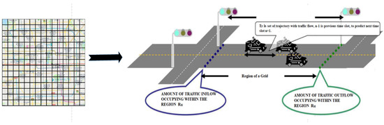
The traffic flow is dynamic; traffic flow always considers the time-dependent data. The higher accuracy is achieved when we consider spatio-temporal data. The traffic flow tensors are { in the grid region R and the previous time slot . The main objective in our problem statement is to predict the citywide traffic flow tensor , where is the next time slot. In Figure 1, we illustrate the problem statement.
Figure 1.
In the left part, we divide the region into the tiny grids, and the right side represents the set of trajectories with inflow and outflow of a region.
4. Materials and Methods
In our approach, Figure 2 illustrates the framework of our proposed model 3DCNN(MBSTALRU). We first initialize the historical data with three different time axes as shown in Figure 3, which are related to the future prediction situation. In the second stage, the spatial and temporal dependency learn 3D CNN stack simultaneously. 3D CNN extracted the common spatial-temporal features related to two tasks: citywide traffic inflow and outflow prediction. In the third stage, we embed spatial-temporal features through attention-based LSTM into a tensor. The spatial-temporal based information tensor fed into the residual layers. Then this information transforms into a vector. Meanwhile, the external information occupies the external branch. For instance, meteorological features are also encoded into the vector [22]. Finally, the two vectors described above are concatenated at the same time to estimate the city-wide traffic flow at the next interval.
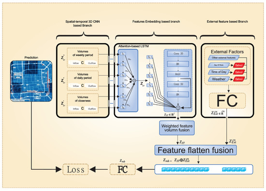
Figure 2.
The Proposed architecture 3DCNN(MBSTALRU).
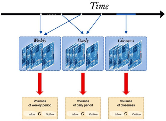
Figure 3.
Modeling of multiple spatial-temporal 3D volumes with multiple spatial-temporal dependencies.
There are 6 components of our multi-branching model 3DCNN(MBSTALRU), where each component is working as follows.
- 3D CNN modeling extracts the information from spatial-temporal data; we present 3D data into the multiple spatial-temporal correlation factors.
- We influence the 3D convolutional block with multiple temporal dependencies. Periodic temporal dependencies have an important role and also affect the future states.
- Spatial-temporal feature extraction with 3D CNN branch, related to two tasks, inflow and outflow of the traffic.
- Extraction of feature embedding branch, the spatial-temporal 3D data are fused into a tensor, and the tensor is represented as .
- External feature-based branch, the external factor data, such as weather conditions, holidays, etc. We encode into the vector .
- We used 3D volumes to train our model 3DCNN(MBSTALRU).
4.1. 3D CNN Modeling with 3-Dimensional Data
In this section, we present our model associated with 3D data. In our model, we present the citywide traffic flow with multiple spatial-temporal dependencies. We present 3D data into the multiple spatial-temporal correlation factors. A tensor that denotes the traffic flow situation of a city in time interval t is . The whole city is separated into an grid map, and k is the number of variables. As shown in Figure 4a, the number of variables k can be considered an image of k channels. The illustration of the kth channel has h pixels height and w pixels width. As the citywide traffic flow point of view states, the multi-channel image preserves the spatial dependencies. We take the traffic situation inflow and outflow in our modeling by setting the channel . In this way, inflow and outflow values are filling by these two channels. These two channels capture the spatial correlations as a citywide traffic flow. The traffic flow values in the given time interval d can be denoted as tensor . As shown in Figure 4b, the constructed tensor represents the 3D data. In this way, a tensor can be considered 3D volume data with a size of , where d is the number of images [21]. The spatial-temporal information of the citywide traffic flow situation can present by the reconstructed 3D data.
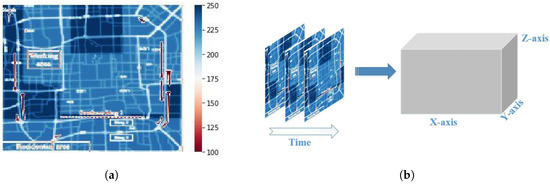
Figure 4.
(a) Traffic inflow/outflow present in a multi-channel image. (b) Slice of the multi-channel image denotes multi-channel 3D volume along with time dimension.
4.2. Multiple Temporal Dependencies
In the recent time, the future states are affected by the historical traffic states. The periodic temporal dependencies have an important role, also affected the future states. For the inflow value of both datasets TaxiBJ and BikeNYC, there are 7 days at each time interval. These figures help find the repeatability pattern in traffic flow data; moreover, they showed the weekly periodicity of traffic flow with repeatability pattern. Illustrated from above, the traffic states have a significant impact based on daily periodicity and weekly periodicity. However, the degree of influence is entirely dissimilar. The traffic states in the recent time have a great impact on the traffic states in the following time. Inspired by the observations, for the multiple temporal properties, we can construct the 3D volume data separately—this separates image-based data of spatial information. For the closeness periodicity 3D volume data, we used a few 2 channel images to model the temporal closeness dependency [22]. Let the traffic flow states be . We have used these fragments in our model with 3D volume data, . According to the same fashion, we can reconstruct the period’s volumes. As an example, we consider the daily period. Suppose the time interval , where d is the period span [25]. The dependent sequence of the daily period is . Per the criteria mentioned above, we can reconstruct the 3D volume . In our implementation, we only used the daily and weekly periods. In the same way, we can construct the other periods, for instance, monthly and seasonal.
4.3. 3D CNN Branch-Based Spatial-Temporal Features Extraction
In this section, the citywide traffic is related to two tasks, inflow and outflow of the traffic. To predict the traffic flow, we trained our model together and inflow and outflow separately. As compared to the previous study, we extract data from the taxi pick-up and drop-off data in time interval t. We scale the data between 0 and 1. We set 0 for inflow and 1 for outflow. In this way, the feature extraction in this stage got the shared information to forecast citywide traffic flow simultaneously. The 3D volume data are expressed as for inflow and for outflow.
Moreover, the adjacent area of a city is affected by each other during the traffic mobility. Thus, the prediction for the potential flow of traffic is based on the historical flow of traffic. This problem has some common ground with video generation, with some pixels and each frame impacting each other. In the field of human action recognition [52] and the video analysis [53], the success of 3D CNN is motivated by the research to utilize the 3D CNN. In our approach, 3D CNN is the primary branch of the multi-branch model. In the structure of CNN, the hidden layer of CNN typically consists of sequences of pooling layers and convolutional layers. The CNN has different levels to extract the features. The CNN has a higher and lower-level of layer interactions. In this way, the higher-level features of the higher layers are reached by integrating the lower-level extracts of the lower layers. Reference [21] visualized CNN with eight layers and this experiment showed the results utilize lower layers that could detect the corner, edges, etc. The visualization results of the higher layer may be used to detect handles, faces, bottles, etc. The pooling layers are concerned, the key objective of these layers is to decrease the number of parameters and computation, to reduce the spatial volume of the function map, and finally to control overfitting [22].
In our study, to obtain the complex spatial-temporal features, we constructed K- 3D convolutional. In convolution operation, we used the zero-padding of input tensor in the first K-. On the other hand, this ensures that the convolutional process covered the edges of the tensor many times. In addition, it entirely captures the interaction between each region of the city as a whole, with the size of the feature map unchanged during the convolutionary operation. In addition, there are few places far away from each other, maybe linked by the metro. Thus, the flow pattern makes these locations appropriate. In our analysis, not only did we reduce the size of the function map and also capture remote dependencies, but we also implement dilated convolution. To manage the high quality of the feature map and remote dependencies, we increased the stride size of the last layer [11].
From a global perspective, to extract the citywide traffic flow, we constructed a three K- 3D CNN. These K- extract the features from the periodicity closeness daily and weekly. We illustrated, to capture the historical data, periodicity closeness as an example. As input tensor and , K- successively followed the convolution as:
is the batch normalization operation, * is the convolutional operation followed by an activation function that is . In the above equation, and are learnable parameters in , and is or .
4.4. Features Embedding Branch Extraction
Based on the 3D CNN, the tensioner has six features that can be interpreted as time series. We suggested an attention-based mechanism for LSTM. The purpose of the attention-based LSTM is to encode the feature tensors into another tensor. The LSTM architecture is a type of RNN [11]. For the processing of time series problems, LSTM is a good option. It was proposed to explore the classic RNN problems or address the gradient vanishing problem.
As shown in the proposed architecture Figure 3, the output of 3D CNN in each time interval t was taken as the input of LSTM after flattening. The peculiar thing about LSTM is it has three gates and memory cells [54]. The names of the three gates are: input gate, forget gate, and output gate [54]. Inside the LSTM structure, information is stored in the memory cell. The purpose of the forget gate is to decide which information passes through the memory cell. The goal of the input gate is to determine what kind of information is added to the cell. The task of the output gate in the next time interval controls the information, and manages what information is referred to next. The input vector is and the output vector is in the time interval t [21]. The input and output vectors are the previous intervals. These intervals were first sent into the forget gate. The forget gate attains the forget gate activation vector . In the following phase, the input gate merges the input and output . The combined values calculate the activation vector . Through activation vectors, we can update the memory cell into . At the previous time interval, the memory cell state vector is . Afterward, the output gates are utilized to find the activation vector with the help of and . Finally, through and at time interval t, we can get the output vector . Formally, the LSTM equations are defined as:
In the above equations, is the hyperbolic tangent function, is the sigmoid function [55], and ∘ is the Hadamard product. The parameters W and bias b are to be learned with different kernel matrices. When LSTM receives the input , from the generated states , we capture the different time intervals to capture the interaction between traffic inflow and outflow. The hidden states of the LSTM are based on the attention mechanism. We have decoded these hidden states to generate the six new vectors. The hidden states are illustrated in the features embedding branch of the main-frame architecture Figure 3, in each timestamp t. We need first to calculate the importance of the extent . We calculate the extent between the hidden states and the previous output of the decoder LSTM. In the next stage, was normalized it into . Finally, can calculate the weighted sum of the hidden state and . The weighted sum gives the context value to be sent to the next timestamp. The hidden state decoding formula is as follows:
In the above equations, is the one-dimensional convolutional network. The other component of the proposed system is trained with this network. We aimed to capture the correlation between traffic inflow and outflow. The deeper network is complicated to train, and we follow the [20] strategy, where authors proposed the residual learning framework. In this way, the residual layers are captured by the correlation mentioned above. Initially, we reshape the six vectors. These vectors come from the attention-based LSTM, and are in the form of matrices. We stacked the vectors into a tensor . In the second stage, we took the tensor as input L. The input L is stacked with residual layers, and can be defined as:
In the above equation, F is the residual units, and the learnable parameter is . Finally, the output of residual layers flattened into a final representation vector .
4.5. External Feature-Based Branch
In this section, external factors can affect the citywide traffic flow states significantly. The example of external factors are holidays, special events, and weather conditions. For instance, during the holidays, such as Christmas and Chinese New Year, some of the regions have more massive traffic flow compared to the non-holidays, while traffic flow situations are opposite in some of the areas. The rainy day is another example of an external factor. Due to slippery roads, the cause can slow down the traffic speed. In the external features-based branch, we mainly consider the holiday events, weather conditions, and other metadata, such as workday and weekend as the example of the day of the week. The multiple temporal dependencies influence the region of the whole city. The different temporal dependencies may be a different degree of influence. We propose a novel method of the multi-branching tensor-based parametric fusion. In our External factor branch, we utilize that the external data have two types: categorical data, such as day of the week, holiday, or weather; numerical data, such as temperature, humidity, or wind speed. In our approach, we conduct one-hot coding for categorical data and stacked them into a vector , while numerical data directly are normalized and stacked into a vector . Finally, concatenate through a fully connected layer . We extracted the spatial-temporal features by the 3D CNN branch, and the feature embedding branch with attention-based LSTM and residual layer unit, stacked them into a vector . Finally, concatenate with the external branch factor . We flattened it into a vector term multi-branch . More specifically, we define:
In the above equations, ∈, , , and are the spatial-temporal features and external features volume extracted by the periodic layers closeness, daily, and weekly. is the two fully connected neural networks, ⨁ indicates the concatenation operator, and ∘ is the Hadamard product. The learnable parameters are , , and ; these parameters adjust the weight of the branches. is the volume of the fusion-based feature. After that, the fully connected layers output towards the prediction component. The prediction component is defined as:
In the above equation, is the ReLU function, and W and b are the learnable parameters [39,56].
4.6. Training Process of the Model
Algorithm 1 illustrates the training of 3DCNN(MBSTALRU). In our training process, the inflow and outflow values in time interval t with images, are regarded as the ground-truth. From the historical traffic states, we constructed a 3D volume of data to utilize as the input of 3DCNN(MBSTALRU). In our implementation, we adopt the closeness branch, daily, and weekly, as periods. The additional periods are considered in the same fashion. We initialized all the trainable parameters proposed in the 3DCNN(MBSTALRU). We randomly use these parameters and then optimize them by backpropagation. To reduce the function of cross-entropy of 3DCNN(MBSTALRU), we adopt the Stochastic Gradient Descent (SGD) [54].
| Algorithm 1 3DCNN(MBSTALRU) Training algorithm |
|
5. Results
In the Section 5, we briefly explain the simulation-based settings and compare them with previous approaches.
5.1. Datasets
We have used two different real-world datasets: BJTaxi and NYCBike. Both datasets have sub-datasets about trajectories and weather details as explained in following subsections. We have implemented our method on Keras (2.1.6) and TensorFlow (1.2.1), with a Nvidia 2060 graphic card. The dataset description is also given below in Table 1.

Table 1.
Statistics of BJTaxi and NYCBike datasets.
5.1.1. BJTaxi
Taxicabs in Beijing have GPS, and we have used the taxicab GPS data in parallel with the meteorology data. The data from Beijing taxicab have four-time intervals. The first interval is 1st July 2013 to 30th October 2013, the 2nd interval is from 1st March 2014 to 30th June 2014, the 3rd interval is from 1st March 2015 to 30th June 2015, and the last interval is 1st November to 2015 to 10th April 2016. We have chosen the last four-weeks data as test data, and all reaming data are taken as training data. We have a 30 min time span in BJTaxi datasets, and we use a grid size [57].
5.1.2. NYCBike
The dataset NYCBike has the data about the trajectory from 1st April to 30th September in 2014. The NYCBike dataset has the following attributes: trip duration, starting and ending stations ID, and start and end times. In all the intervals of the NYCBike dataset, we have chosen the last ten days from the intervals as test data, all the remaining data were selected as training data. For this dataset, we take the timespan as 60 min. We take the grid size of . The dataset is available on the Kaggle dataset website [58].
5.2. Model Implementation Details
In this section, we briefly explain the model implementation details.
5.2.1. Data Preprocessing
In the preprocessing part, we break up the entire city into a grid map for the BjTaxi dataset. We fragmented the city as the whole into an grid map for the NYCBike dataset. We set the period for BJTaxi to 30 min, and NYCBike to 1 h. Using Definition 2 and both datasets BJTaxi and NYCBike, we can get two types of traffic flows. The features such as weekday or weekend, day of the week, holidays, weather conditions, and other metadata, are transformed into the binary vectors. Then binary vectors are fed into the framework of the external factors. The original value of the traffic is scaling between (0,1) with minimum and maximum normalization. For the evaluations, prediction values are denormalized. In this way, before comparing our proposed method with the existing method to make a fair comparison, we also apply the minimum and maximum normalization to the baseline method [57,58].
5.2.2. Parameter Tuning
On the dataset NYCBike, the number of time intervals of closeness, daily, weekly are 4, 4, and 4, respectively. On the dataset BJTaxi, the number of time intervals of closeness, daily, and weekly, are 6, 4, and 4, respectively. The timestamp of NYCBike is 1 h, and BJTaxi is a half-hour. We put the learning rate for all models to . We optimize the model to apply the Adam optimizer. We trained the proposed models with a maximum training iteration of 200 epochs and used an early stopping strategy. The purpose of early stopping is to stop training if the loss of validation for 15 consecutive epochs does not decrease [46]. In addition, we used ReLu for all layers as an activation function. During the experiment, we set a batch size 64 for batch normalization.
Two important factors we need to follow when designing the structure of neural networks are: (1) depth of the network, and (2) convolutional layer hyperparameters and pooling layer. In the second factor, be careful about the filter size of the convolutional layer and pooling size. The NYCBike dataset, owing to the size we set our generated 3 dimension, is small, i.e., . In all branches for NYCBike, we selected only two 3D CNN layers. The kernel size is set (2,2,3) in all branches. The expression 2 in kernel size denotes the temporal kernel size, and the reaming term (2,3) denotes the spatial kernel size. The first layer consists of 32 3D convolutional filters, and the second layer is 64. The gate of LSTM set spatial-temporal kernel size (2,2,3) is applied. The spatial-temporal kernel’s goal is to control the spatial-temporal features. The size of the pooling layer is charged with the size (1,2,2) is followed. The additional dropout layer is set to solve the problem of over-fitting. The size of the additional dropout layer is 0.25.
In the second real-world dataset BJTaxi, we partition the grid map into . The grid map of the BJTaxi is larger than the dataset NYCBike. In all multiple branches, we apply three 3D CNN layers. We describe the parameters of our model (MBSTRU) and (MBSTAL) as follows. The kernel size is set to (2,2,3) for the closeness branch for these three layers. The other two branches, like daily and weekly, set the kernel size (2,2,3) for the first layer, while we set (1,2,3) kernel size for the other two layers. The purpose of the above settings is to align the output size of the branches’ closeness, daily, and weekly. We set the number of 3D convolutional filters to 32, 64, and 64 for three 3D CNN layers, respectively. The LSTM gates have spatial-temporal feature information and also follows these three layers. The gate controls the flow of spatial-temporal features with the kernel (2,2,3). The max-pooling layer and dropout layer parameters are like those for the NYCBike dataset. In the spatial-temporal CNN block, we adopt the residual fusion mechanism.
Evaluation metrics: We use root mean square error (RMSE) in the evaluation. Formally, the RMSE is defined as follows:
N is the number of all samples in time interval t, denotes the real value, and the predicted value.
5.3. Baseline Models
Our 3DCNN(MBSTALRU) is compared with nine baselines as follows.
Prediction Approaches concerning Classical Time-series Models:
- HA: Historical average, we predict the average from historical values in the simulation process. This is a very basic model in the baseline steps [20].
- ARIMA: In the time series forecasting problem, the ARIMA model is a well-known model to predict about the future vales of time series [19].
Prediction Approaches concerning Classical Statistical Models:
- XGBoost [10]: XGBoost is a famous tree method, boosts the performance.
- LinUOTD [59]: This method is based on the linear regression method. This linear regression method works with spatial-temporal regularization.
Prediction Approaches concerning Deep Learning Models:
- Multilayer Perception (MLP): MLP is a neural network; the implementation of this method uses four fully connected layers [15,16].
- ConvLSTM: In this method, add convolutional layers with LSTM [14].
- ST-ResNet: This method uses 2D images to models the citywide traffic flow at a different time interval. The ST-ResNet extracts the spatial features to utilize 2D CNN. The ResNet model utilizes the closeness, period, and trend information to predict the traffic flow [6]. In the ResNet model, aggregate the relevant features together to utilize the function tanh. The length trend we set for period and closeness as 4, 4, and 4, respectively.
- STDN: In this method, to predict traffic flow, combine attention mechanism, LSTM, and local 2D CNN. This method we utilize to make the model novel. This method gives us basics knowledge of the implementation of our strategy [51]. We modify the implementation source code of STDN to predict the traffic flow while maintaining the network structure of STDN.
- MGSTC: The framework multi-gated spatial-temporal convolutional. In this work, we adopt the spatial-temporal gated mechanism with the spatial-temporal CNN blocks [21].
We propose our method 3DCNN(MBSTALRU) with three variants. The variants are listed as follows. Our proposed method consists of convolutional, feature embedding, and external branches.
- 3DCNN(MBSTRU): In this variant, we removed the attention-based LSTM, we used the three layers of 3D convolutional with 4 to 8 layers of residual units. We stacked the feature embedding branch into the tensor. The tensor was taken as the input of the residual layers unit.
- 3DCNN(MBSTAL): In our proposed work, we utilize the 3D convolutional branches with the attention-based LSTM layers. The result of the 3D CNN is stacked and fed into the feature embedding branch to extract the features with attention-based LSTM to predict the citywide traffic flow.
- 3DCNN(MBSTALRU): In this variant is the proposed spatial-temporal CNN block to utilize with feature embedding and the external branch to predicting the citywide traffic flow simultaneously.
5.4. Performance Evaluation as Compared to Baseline Methods
In this section, we compared our results with prior baseline approaches. In Table 2, we use valuation RMSE as evaluation matrices; we present our results for traffic inflow and outflow together. In Figure 5, we compare the RMSE results of our model with previous baseline methods. We evaluate our results on two real-world datasets: BJTaxi and NYCBike. Further, we run our proposed model separately for inflow and outflow to get detailed results. We also compared our results with previous baseline methods concerning inflow and outflow traffic flow. We present a detailed comparison of traffic inflow and outflow in Table 3 and Table 4. On the dataset BJTaxi, our proposed variant 3DCNN(MBSTRU) inflow RMSE is 11.49, and outflow is 11.61. The average RMSE is 11.55. On the dataset, NYCBike, inflow RMSE is 4.01 and outflow is 4.26. The average RMSE is 4.13. In our second variant, 3DCNN(MBSTAL), we add attention-based LSTM, the RMSE is further decreased. On the dataset BJTaxi, our proposed variant 3DCNN(MBSTAL), inflow RMSE is 11.20 and outflow is 11.42. The average RMSE is 11.31. On the dataset, NYCBike, inflow RMSE is 3.85 and outflow is 4.16. The average RMSE is 4.00. In Table 3 and Table 4, we present more details of the inflow and outflow of traffic flow. Our variant 3DCNN(MBSTRU) is outperforming as compared to the previous baseline methods. We combine all 3D CNN branches with the residual layer units results that are more effective. We extract the spatial-temporal features, merge the feature embedding branch with the external feature branch, and compare it with the previous model. We also note that our attention-based LSTM variants outperform residual unit variants.
Table 2.
Baseline comparison on BJTaxi and NYCBike datasets.
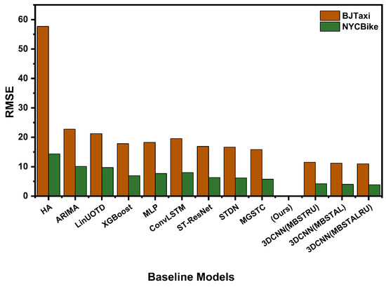
Figure 5.
RMSE comparison on BJTaxi and NYCBike datasets.
Table 3.
Dataset BJTaxi inflow/outflow comparison.
Table 4.
Dataset NCYBike inflow/outflow comparison.
Furthermore, our variant in which we combine attention-based LSTM and the residual unit, outperforms our two variants. The variant 3DCNN(MBSTALRU) is outperforming RMSE compared to the previous baseline methods. The performance of our variants indicates we effectively extract the spatial-temporal characteristics for traffic mobility data. If we examine Table 2, Table 3 and Table 4, we can conclude that the 3DCNN(MBSTALRU) outperforms 3DCNN(MBSTRU) and 3DCNN(MBSTAL). We effectively adapt the multi-branching mechanism to increase the accuracy of the model.
In contrast, from the details we represented in Table 2, Table 3 and Table 4, the traditional time series model does not achieve excellent performance. In Figure 6 and Figure 7, we visualize the RMSE of inflow and outflow comparison with previous baseline methods on BJTaxi and NYCBike datasets. The traditional models, such as ARIMA and HA, only explore the traffic prediction based on historical values. These models do not utilize the spatial-temporal features and external factors. The regression method performs very well if we compare the results with traditional methods. The regression method explores the spatial correlations. The drawback of the regression method is it also fails to capture spatial and temporal dependence completely.
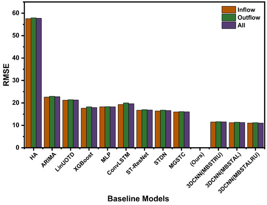
Figure 6.
RMSE of inflow and outflow comparison with baseline methods on BJTaxi dataset.
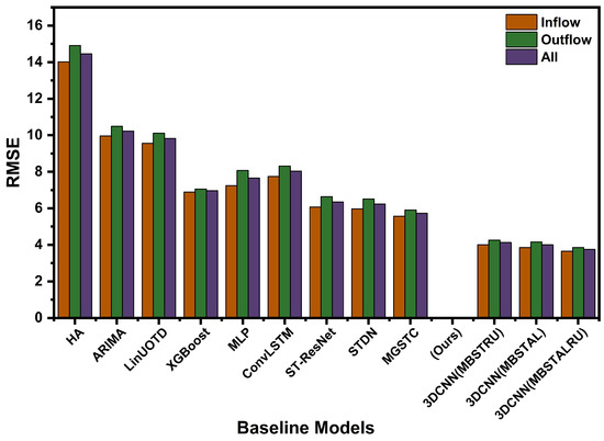
Figure 7.
RMSE of inflow and outflow comparison with baseline methods on the NYCBike dataset.
Our proposed method outperforms MLP, ST-ResNet, and MGSTC. The possible reason may be MLP does not explicitly capture the spatial-temporal dependencies. The limitation of ResNet is this method only uses the 2D CNN to learn the low-level spatial features. For the temporal dependencies, take advantage of the tanh function. The MGSTC uses the multi-gated method to capture the spatial and temporal dependencies, but one of the potential reasons that the outcome is lower than our method is the time delay between input and output. Our variants perform state-of-the-art results as compared to the ConvLSTM and STDN. In this method, we adopt 2D CNN combined with LSTM together, to capture the spatial and temporal dependencies from low-level spatial feature learning.
5.5. Impact of Residual Fusion
To make the final output simultaneously and make the output of spatial and temporal convolutional influence, we have adopted the residual connection. We utilize the residual connection between the outcome of the spatial-temporal convolutional block, and the output of spatial convolutional. For the output of the spatial and temporal convolutional, we evaluate the residual fusion in this section. The adoption of residual connection can be observed in Table 5. When increase the depth of the residual layers we get variations in the results. Increase the number of residual layers decreases RMSE, but we train until results increase. In our approach, we used 4 to 8 residual layers.
Table 5.
Impact of residual fusion and attention-based LSTM.
5.6. Impact of Attention-Based LSTM
The attention-based LSTM variant 3DCNN(MBSTAL) has more impact as compared to the MBSTRU variant. In Table 5, we consider the BJTaxi and NYCBike datasets with variations due to attention-based LSTM. The RMSE is 11.13 and 3.88. Technically, LSTM is an excellent neural network for processing the time series problem. The way to tackle critical information is attention mechanism mimics the way. We fuse the spatial-temporal features from the historical traffic flow. We combine attention mechanisms with LSTM. In Table 3 and Table 4 we present the detailed inflow and outflow of traffic flow, the RMSE of inflow and outflow on BJTaxi and NYCBike datasets. LSTM considers the spatial and temporal correlation. The attention mechanism is to assign the weights—setting the weights to represent the new representation of historical data.
5.7. Effects of Multi-Branches Features
In this section, we evaluate the effect of adopting multi-branching 3D CNN. We also evaluate the effectiveness of external factors. In our variants, we apply the different branches as follows:
3DCNN(MBSALRU)-CB: In this variant, on spatial-temporal convolutional blocks with attention-based LSTM and residual function, only utilize the closeness branch (CB).
3DCNN(MBSALRU)-CDB: In this variant, on spatial-temporal convolutional blocks with attention-based LSTM and residual function, only utilize the closeness and daily branches (CDB).
3DCNN(MBSALRU)-CDWB: In this variant, on spatial-temporal convolutional blocks with attention-based LSTM and residual function, only utilize the closeness, daily, and weekly branches (CDWB).
Our proposed model, 3DCNN(MBSTALRU), shows the results with its variants. We observe that our variant 3DCNN(MBSTALRU)-CB uses only the closeness branch to outperform compared to other baseline methods. It validates the benefit of utilizing the 3D CNN branch to learn the spatial-temporal features. We used two real-world datasets to predict citywide traffic flow with different branches. We can observe in daily and weekly branches, RMSE further decreases. In this way, we conclude that the prediction performance increases if we increase the periodic dependencies. In the BJTaxi dataset, we can examine the RMSE of closeness, and the daily branch is bigger than the RMSE of the daily branch. For the BJTaxi dataset, the daily branch has little effect. We can increase the performance by adding the external feature branch. At the final stage, we can observe the RMSE result is lowest when we combine all branches with the external feature branch.
5.8. Time Complexity Analysis with Different Approaches
In this section, we compare the time complexity of our proposed variants 3DCNN(MBSTRU), 3DCNN(MBSTAL), and 3DCNN(MBSTALRU) with previous baseline methods. In Table 6, we present the training and testing times. We utilized the Nvidia 2080 12 GB to process all the approaches. Our proposed method, 3DCNN(MBSTALRU), achieved good results. We only compared the method with ResNet, STDN, and MGSTC. We noticed that the STDN and ResNet training and testing times are the longest. The reason for the longest training time is that STDN utilizes the local CNN and local CNN only predicts the center of the values. The second reason is STDN uses the sliding window across the whole city. In the sliding window train, the entire city then predicts every region of the city. For example, in the NYCBike dataset, it needs to repeat 8 × 16 times traffic values to predict the entire city for the NYCBike dataset. If we consider the BJTaxi dataset, our proposed method, 3DCNN(MBSTALRU), performs very well compared to ResNet. The main reason is that ResNet uses only two convolutional layers and 12 residual units. In our approach, we use two 3D CNN layers and 8 residual units. The approach MGSTC uses the multiple gated mechanisms, time delay occupied between input and output. Our proposed variant training and testing times are less, and we adopt 3D CNN with spatial-temporal convolutional branches, feature embedding, and external branches. Our proposed method achieves the best results and less training and testing time.
Table 6.
Time complexity comparison of different methods.
6. Discussion and Conclusions
We proposed a citywide traffic flow prediction method to predict simultaneously, and the impact of studies forecasting, traffic flow on the accuracy of inflow and outflow of traffic on two real-world datasets. Then, we obtained the findings below:
- Traffic congestion is one of the serious problems among many cities, such as Beijing and New York. These cities face many different pressures and challenges, like waiting time, low car speed, long traveling, etc. To forecast traffic flows in cities, many researchers attempt to influence deep learning-based methods.
- Based on the 3DCNN(MBSTALRU) methods, including spatial-temporal information, the RMSE of traffic flow together is 10.99. We train our model to simulate the inflow and outflow results separately. The average RMSE of inflow and outflow on BJTaxi is 11.1. The RMSE increases 0.11 when we simulate the inflow and outflow separately. On NYCBike dataset, we simulate the traffic flow together and RMSE is 3.85. The average result of RMSE as inflow and outflow is 3.75. The RMSE is decreased by 0.10, as shown in Figure 6. In the previous study, MGSTC outperforms as compared to previous baseline methods. Our model 3DCNN(MBSTALRU) outperforms by 55% as compared to MGSTC and by 60% as compared to the STDN.
- For our proposed variants 3DCNN(MBSTRU), 3DCNN(MBSTAL), and 3DCNN(MBSTALRU), the RMSE of 3DCNN(MBSTAL) decreases 0.29 as compared to 3DCNN(MBSTRU) on the BJTaxi dataset. The RMSE of 3DCNN(MBSTALRU) decreases by 0.21 as compared to 3DCNN(MBSTAL) variants. Similarly, for the NYCDataset, the RMSE of 3DCNN(MBSTAL) decreases by 0.23 as compared to 3DCNN(MbSTRU). The RMSE of 3DCNN(MBSTRUAL) improves by 0.13 as compared to 3DCNN(MBSTAL).
- Multi-branch features also create variations on the simulation results. We utilize the closeness branch (CB). We merge closeness with the daily branch (CDB), and finally, we merge them with the weekly branch (CDWB). The prediction accuracy improved. The 3DCNN(MBSTRU) RMSE is increased by 0.24 and 0.06 on BJTaxi and NYCBike datasets. Similarly, variant 3DCNN(MBStAL) is increased by 0.07 and 0.10. Finally, on the variant 3DCNN(MBSTALRU), RMSE increased by 0.08 and 0.05. Our main variant 3DCNN(MBSTALRU) outperforms all previous methods defined in the baseline methods.
- We also explore the impact of attention-based LSTM, residual layers unit with 3D CNN convolutional block. We combine 3D CNN with residual layers unit, the average RMSE 11.60; later, we combine 3D CNN with attention-based LSTM, RMSE improves 0.31,. In this way, we combine attention-based LSTM and residual layers with 3D CNN, accuracy improves 0.31 to 0.60 as shown in Figure 7 and Figure 8.
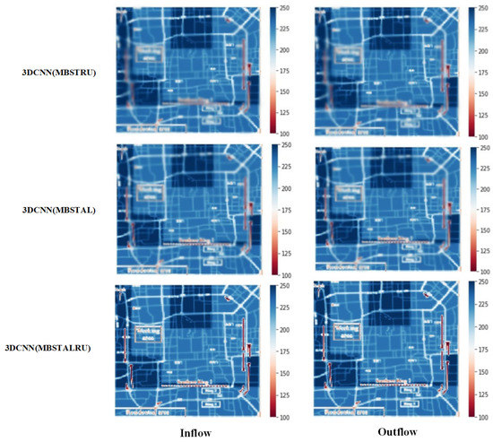 Figure 8. For the dataset BjTaxi, visual comparison of different variants. The left column is the inflow, and the right column is the outflow.
 - Traffic congestion is occupied mostly morning, noon, and evening time. Let us examine some at 8:30 a.m, some at 8:50. a.m, some at 9:00 a.m and some at 9:30 a.m. Most of them spent significant time on roads in the traffic jam. In modern cities, facing the most critical problem is traffic congestion. The economist estimates the cost related to traffic congestion in 2017 in the UK, US, and Germany was 461$. We can use artificial intelligence technologies to reduce the traffic congestion and reduce the cost related to traffic congestion. For example, we can use a machine-learning algorithm to design a real-time traffic signal control system, utilizing cameras placed at the road intersections. Intelligent traffic signals optimize the road traffic such as less waiting time, shorter trips, reduced traffic congestion, less pollution, and happier drivers.
Limitation of the Study. The research still has some limitations. In the future, these limitations should be studied. For example, we will use real-time location-based social network website data such as FourSquare to make prediction accuracy more real-time. Additionally, we should propose a method covering traffic flow prediction with travel time estimation, origin-destination with graph data, or traffic flow prediction with the mobility on demand (MOD). Moreover, we should increase the evaluation matrices to validate the results from different angles. In this research article, our finding are to predict traffic flow, to reduce traffic congestion. Our model predicts accurately compared to previous methods, but in real-life practice, we still have some gaps. For example, traffic congestion creates a deadlock in traffic flow, traveling waiting time increases, the health of the public is psychologically affected by the waiting on the road, environmental pollution increases, and transportation fails to deliver goods on time. We can use artificial intelligence technologies to reduce the traffic congestion and reduce the cost of traffic congestion.
Major Concern of Traffic based on Artificial intelligence and Deep Learning Methodology. Our proposed methodology is based on traffic AD terminology and refers to artificial intelligence (AI) and deep learning (DL) applications. We can apply traffic infrastructure traffic AD due to its capabilities to collect traffic data, analyze it, and create solutions. The traffic optimization problem is solved with government bodies, universities, and different organizations. Traffic AD is still experimental. Traffic AD systems currently offer cities the authority to enhance traffic management and monitoring of traffic volume. A secure, stable traffic AD can be able to monitor traffic flow in the future autonomously. Traffic AD operates by collecting information from related traffic flow systems that deliver input on live traffic or historical traffic behavior. It uses deep learning approaches to process, understand, and learn about traffic infrastructure to comprehend this unstructured traffic volume. To solve traffic congestion, the AD then uses these observations.
Traffic AD systems, including photographs and videos, are proficient in processing and analyzing various data kinds. Traffic AD systems, aided by computer vision techniques, can identify objects from traffic cameras in images and videos by breaking them down into characteristics and matching them to modules like “car,” “bike,” or “pedestrian.”
Objects classifications and detection can differentiate between cars and pedestrians, between unlike vehicle kinds, and between buildings and living beings. Traffic AD can count vehicles, assess and re-route traffic accordingly if a road is congested.
At a certain point, traffic AD will begin detecting trends to well understand the traffic environment after accumulating enough data. It can learn to distinguish between incidents, such as a rush-hour or car accident, that may cause congestion. It may conduct the predictive investigation and use the knowledge to enhance traffic movement as traffic AD discovers at which times rush hour occurs.
Use Cases of Traffic AD. We can practice traffic AD to enhance the traffic flow and benefits for drivers as follows.
Traffic Patterns. Traffic AD systems can detect traffic trends using predictive analytics and avoid or mitigate road congestion before it occurs. Through their ITS, smart cities may incorporate a traffic AD system, or construct the AD into their advanced traffic management system (ATMS).
Traffic Lights. Traffic AD systems can optimize traffic lights and reduce intersection waiting times. In images from traffic cameras, the AD detects cars. The traffic data are sent to a control center, where algorithms analyze traffic compactness. It can go through traffic lights to re-route traffic flow, based on real-time information, if the system detects congestion.
Improved Safety. Emergency services and public transport can be made safer and more efficient by traffic AD systems. Traffic AD differentiates between road user types and can accordingly prioritize the flow of traffic. When the commercial identifies an emergency vehicle to reach their destination more quickly, it can re-route traffic to help emergency responders. The AD will enable it to make a stop on time if a bus is stuck in traffic.
Traffic AD with Superhuman Traffic Controller. We could have every road and intersection watched by a city transportation official or police officer, and make real-time decisions to improve traffic flow situations. This would be difficult to do with individuals, but with AD traffic today, it is a reality. The capability to track enormous data capacities in real-time and make smart decisions will have a massive effect on congested cities, above and beyond what conventional analytics have previously achieved. According to data-driven insights, the greater the traffic efficiency effect, the further AD is permitted to function openly, re-routing traffic. AD can, however, create errors that have unintentional significance. Transportation policymakers would need to follow a sensible approach to implementing AD that permits the traffic flow system to learn on a magnitude while keeping human interference controls in place.
Conclusions
The traffic forecast problem is very challenging. This problem consists of many complex factors. The complex factors included multiple spatial-based dependencies and the temporal-based dependencies. To make the prediction accurate, with spatial-temporal correlations, also external factors influence it. Across the whole neural network stack, to extract the spatial-temporal features, we proposed the spatial-temporal-based convolutional block. In the first level, we proposed a novel multi-branch-based model, and the model utilized 3D CNN with different periodicity branches to extract the spatial-temporal features. In the second level, our feature embedding branch consists of the attention-based LSTM to embed the features and combine with the units of the residual layer. The feature embedding branch captures the inflow and outflow of the citywide traffic flow. The external factor branch contains some external factors to make an influence on the traffic flow. In this way, to make predictions more accurate than the previous baseline method, fused with external factors. Our task is to predict simultaneously, our spatial-temporal convolutional branch capture the multiple spatial and temporal dependency together with external factors. Our prediction accuracy is improved 55% to 60% as compared to previous baseline methods. However, our study is still not perfect and has some limitations. From the following aspects, as a future study point of view, we will consider improving our accuracy more. We will explore more graphical knowledge of road networks, calculate travel time estimation, and route recovery with citywide traffic flow. We will divide the city-states according to semantic states. We will include the impact of COVID-19 in the traffic flow.
Author Contributions
Conceptualization, Z.U.A., H.S., and Z.Y.; funding acquisition, H.S.; methodology, Z.U.A., H.S., and Z.Y.; project administration, Z.U.A.; resources, H.S.; software, Z.Y. and A.A.; supervision, H.S. and Z.Y.; validation, Z.U.A., H.S., and Z.Y.; visualization, Z.U.A.; writing—original draft, Z.U.A. and A.A.; writing—review and editing, Z.U.A., H.S., Z.Y., and A.A. All authors have read and agreed to the published version of the manuscript.
Funding
The work sported by the National Science Foundation of China grants 61672417 and 61876138, and Shaanxi key research and development program 2020KW-002. Any opinions, findings, and conclusions expressed here are those of the authors and do not necessarily reflect the views of the funding agencies..
Acknowledgments
Data retrieved from Kaggle and T-drive-trajectory.
Conflicts of Interest
The authors declare no conflict of interest.
Abbreviations
The following abbreviations are used in this manuscript:
| MBSTALRU | Multi-Branching Spatial-Temporal Attention-based Long-Short term Memory |
| LSTM | Long-Short term Memory |
| CNN | Convolutional Neural Networks |
| ITS | Intelligent Transportation System |
| GPS | Global Positioning System |
| UN | United Nation |
| SVR | Support Vector Regression |
| KF | Kalman Filters |
| ARIMA | Auto-Regressive Integrated Moving Average |
| K-NN | K-Nearest Neighbors |
| RF | Random Forest |
| ANN | Artificial Neural Network |
| NLP | Nature Language Processing |
| CV | Computer Vision |
| RNNs | Recurrent Neural Networks |
| MLT | Multi-Tasking Learning |
| ST-ResNet | Spatial-Temporal Residual Network |
| GRU | Gated Recurrent Unit |
| ConLSTM | Convolutional Long-term Short-term Memory |
| HMM | Hidden Markov Model |
| GMM | Gaussian Mixture Model |
| FC | Fully Connected |
| GRU | Gated Recurrent Unit |
| HA | Historical Average |
| STDN | SPATIAL TEMPORAL DEEP NETWORK |
| MGSTC | MULTI-GATED SPATIAL TEMPORAL CONVOLUTION |
| CB | Closeness Branch |
| CDB | Closeness Daily Branch |
| CDWB | Closeness Daily Weekly Branch |
| AD | Artificial Intelligence and Deep learning |
| ATMS | Advanced Traffic Management System |
References
- Zhang, J.; Wang, F.-Y.; Wang, K.; Lin, W.-H.; Xu, X.; Chen, C. Data-Driven Intelligent Transportation Systems: A Survey. IEEE Trans. Intell. Transp. Syst. 2011, 12, 1624–1639. [Google Scholar] [CrossRef]
- Wang, Y.; Zheng, Y.; Xue, Y. Travel time estimation of a path using sparse trajectories. In Proceedings of the 20th ACM SIGKDD International Conference on Knowledge Discovery and Data Mining, New York, NY, USA, 24–27 August 2014. [Google Scholar]
- Ma, X.; Dai, Z.; He, Z.; Ma, J.; Wang, Y.; Wang, Y. Learning Traffic as Images: A Deep Convolutional Neural Network for Large-Scale Transportation Network Speed Prediction. Sensors 2017, 17, 818. [Google Scholar] [CrossRef] [PubMed]
- Wiseman, Y. Real-Time Monitoring of Traffic Congestions. In Proceedings of the IEEE International Conference on Electro Information Technology (EIT 2017), Lincoln, NE, USA, 14–17 May 2017; pp. 501–505. [Google Scholar]
- United Nations Department of Economics and Social Affairs. World Urbanization Prospects: The 2017 Revision; United Nations Department of Economics and Social Affairs, Population Division: New York, NY, USA, 2018. [Google Scholar]
- Zhang, J.; Zheng, Y.; Qi, D. Deep spatio-temporal residual networks for citywide crowd flows prediction. In Proceedings of the Thirty-First AAAI Conference on Artificial Intelligence, San Francisco, CA, USA, 4–9 February 2017. [Google Scholar]
- Drucker, H.; Burges, C.J.; Kaufman, L.; Smola, A.J.; Vapnik, V. Support vector regression machines. In Advances in Neural Information Processing Systems; MIT Press: Cambridge, MA, USA, 1997; pp. 155–161. [Google Scholar]
- Zhang, L.; Liu, Q.; Yang, W.; Wei, N.; Dong, D. An Improved K-nearest Neighbor Model for Short-term Traffic Flow Prediction. Procedia Soc. Behav. Sci. 2013, 96, 653–662. [Google Scholar] [CrossRef]
- Sun, Y.; Wang, H.; Xue, B.; Jin, Y.; Yen, G.G.; Zhang, M. Surrogate-Assisted Evolutionary Deep Learning Using an End-to-End Random Forest-Based Performance Predictor. IEEE Trans. Evol. Comput. 2019, 24, 350–364. [Google Scholar] [CrossRef]
- Kuchipudi, C.M.; Chien, S.I.J. Development of a Hybrid Model for Dynamic Travel-Time Prediction. Transp. Res. Rec. J. Transp. Res. Board 2003, 1855, 22–31. [Google Scholar] [CrossRef]
- Ma, X.; Tao, Z.; Wang, Y.; Yu, H.; Wang, Y. Long short-term memory neural network for traffic speed prediction using remote microwave sensor data. Transp. Res. Part C Emerg. Technol. 2015, 54, 187–197. [Google Scholar] [CrossRef]
- He, K.; Zhang, X.; Ren, S.; Sun, J. Deep Residual Learning for Image Recognition. In Proceedings of the 2016 IEEE Conference on Computer Vision and Pattern Recognition (CVPR), Las Vegas, NV, USA, 26 June–1 July 2016; pp. 770–778. [Google Scholar]
- Ioannidou, A.; Chatzilari, E.; Nikolopoulos, S.; Kompatsiaris, I. Deep Learning Advances in Computer Vision with 3D Data. ACM Comput. Surv. 2017, 50, 1–38. [Google Scholar] [CrossRef]
- Ghosh, S.; Vinyals, O.; Strope, B.; Roy, S.; Dean, T.; Heck, L. Contextual lstm (clstm) models for large scale nlp tasks. arXiv 2016, arXiv:1602.06291. [Google Scholar]
- Khan, W.; Daud, A.; Nasir, J.A.; Amjad, T. A survey on the state-of-the-art machine learning models in the context of NLP. Kuwait J. Sci. 2016, 43, 95–113. [Google Scholar]
- Aone, C.; Okurowski, M.E.; Gorlinsky, J. Trainable, scalable summarization using robust NLP and machine learning. In Proceedings of the (17th,36th) Annual Meeting of the Association for Computational Linguistics and Computational Linguistics, Montréal, QC, Canada, 10–14 August 1998; Volume 1, pp. 62–66. [Google Scholar]
- Jin, W.; Lin, Y.; Wu, Z.-H.; Wan, H. Spatio-Temporal Recurrent Convolutional Networks for Citywide Short-term Crowd Flows Prediction. In Proceedings of the 2nd International Conference on Computing and Wireless Communication Systems—ICCWCS’17, New York, NY, USA, 14–16 November 2018; pp. 28–35. [Google Scholar]
- Li, Y.; Zheng, Y.; Zhang, H.; Chen, L. Traffic prediction in a bike-sharing system. In Proceedings of the 23rd SIGSPATIAL International Conference on Advances in Geographic Information Systems—GIS ’15, Washington, DC, USA, 3–6 November 2015; p. 33. [Google Scholar]
- Yin, Y.; Chen, L.; Xu, Y.; Wan, J. Location-Aware Service Recommendation with Enhanced Probabilistic Matrix Factorization. IEEE Access 2018, 6, 62815–62825. [Google Scholar] [CrossRef]
- Yin, Y.; Aihua, S.; Min, G.; Xu, Y.S.; Wang, S.P. QoS Prediction for Web Service Recommendation with Network Location-Aware Neighbor Selection. Int. J. Softw. Eng. Knowl. Eng. 2016, 26, 611–632. [Google Scholar] [CrossRef]
- Chen, C.; Li, K.; Teo, S.G.; Zou, X.; Li, K.; Zeng, Z. Citywide Traffic Flow Prediction Based on Multiple Gated Spatio-temporal Convolutional Neural Networks. ACM Trans. Knowl. Discov. Data 2020, 14, 1–23. [Google Scholar] [CrossRef]
- Kuang, L.; Yan, X.; Tan, X.; Li, S.; Yang, X. Predicting Taxi Demand Based on 3D Convolutional Neural Network and Multi-task Learning. Remote Sens. 2019, 11, 1265. [Google Scholar] [CrossRef]
- Abdelaziz, A.; Elhoseny, M.; Salama, A.S.; Riad, A. A machine learning model for improving healthcare services on cloud computing environment. Measurement 2018, 119, 117–128. [Google Scholar] [CrossRef]
- Yin, Y.; Xu, W.; Xu, Y.; Li, H.; Yu, L. Collaborative QoS Prediction for Mobile Service with Data Filtering and SlopeOne Model. Mob. Inf. Syst. 2017, 2017, 7356213. [Google Scholar] [CrossRef]
- Yin, Y.; Xu, Y.; Xu, W.; Gao, M.; Yu, L.; Pei, Y. Collaborative Service Selection via Ensemble Learning in Mixed Mobile Network Environments. Entropy 2017, 19, 358. [Google Scholar] [CrossRef]
- Gao, H.; Miao, H.; Liu, L.; Kai, J.; Zhao, K. Automated Quantitative Verification for Service-Based System Design: A Visualization Transform Tool Perspective. Int. J. Softw. Eng. Knowl. Eng. 2018, 28, 1369–1397. [Google Scholar] [CrossRef]
- Zhao, J.L.; Tanniru, M.R.; Zhang, L.-J. Services computing as the foundation of enterprise agility: Overview of recent advances and introduction to the special issue. Inf. Syst. Front. 2007, 9, 1–8. [Google Scholar] [CrossRef]
- Gao, H.; Chu, D.; Duan, Y.; Yin, Y. Probabilistic Model Checking-Based Service Selection Method for Business Process Modeling. Int. J. Softw. Eng. Knowl. Eng. 2017, 27, 897–923. [Google Scholar] [CrossRef]
- Gao, H.; Huang, W.; Yang, X.; Duan, Y.; Yin, Y. Toward service selection for workflow reconfiguration: An interface-based computing solution. Future Gener. Comput. Syst. 2018, 87, 298–311. [Google Scholar] [CrossRef]
- Abdelaziz, A.; Ahmed, S.; Salama, M. A machine learning model for predicting of chronic kidney disease based internet of things and cloud computing in smart cities. Measurement 2019, 119, 93–114. [Google Scholar]
- Chen, Y.; Deng, S.; Ma, H.; Yin, J. Deploying Data-intensive Applications with Multiple Services Components on Edge. Mob. Netw. Appl. 2019, 25, 426–441. [Google Scholar] [CrossRef]
- Sangaiah, A.K.; Medhane, D.V.; Han, T.; Hossain, M.S.; Amin, S.U. Enforcing Position-Based Confidentiality With Machine Learning Paradigm Through Mobile Edge Computing in Real-Time Industrial Informatics. IEEE Trans. Ind. Inform. 2019, 15, 4189–4196. [Google Scholar] [CrossRef]
- Amodei, D.; Ananthanarayanan, S.; Anubhai, R.; Bai, J.; Battenberg, E.; Case, C.; Casper, J.; Catanzaro, B.; Cheng, Q.; Chen, G.; et al. Deep speech 2: End-to-end speech recognition in english and mandarin. In Proceedings of the International Conference on Machine Learning, New York, NY, USA, 20–22 June 2016; pp. 173–182. [Google Scholar]
- Zhang, Y.; Yang, Q. An overview of multi-task learning. Natl. Sci. Rev. 2017, 5, 30–43. [Google Scholar] [CrossRef]
- Van Der Voort, M.C.; Dougherty, M.; Watson, S. Combining kohonen maps with arima time series models to forecast traffic flow. Transp. Res. Part C Emerg. Technol. 1996, 4, 307–318. [Google Scholar] [CrossRef]
- Williams, B.M. Multivariate Vehicular Traffic Flow Prediction: Evaluation of ARIMAX Modeling. Transp. Res. Rec. J. Transp. Res. Board 2001, 1776, 194–200. [Google Scholar] [CrossRef]
- Hamed, M.M.; Al-Masaeid, H.R.; Said, Z.M.B. Short-Term Prediction of Traffic Volume in Urban Arterials. J. Transp. Eng. 1995, 121, 249–254. [Google Scholar] [CrossRef]
- Wu, C.-H.; Ho, J.-M.; Lee, D. Travel-Time Prediction With Support Vector Regression. IEEE Trans. Intell. Transp. Syst. 2004, 5, 276–281. [Google Scholar] [CrossRef]
- Zheng, W.; Lee, D.-H.; Shi, Q. Short-Term Freeway Traffic Flow Prediction: Bayesian Combined Neural Network Approach. J. Transp. Eng. 2006, 132, 114–121. [Google Scholar] [CrossRef]
- Kuang, L.; Yan, H.; Zhu, Y.; Tu, S.; Fan, X. Predicting duration of traffic accidents based on cost-sensitive Bayesian network and weighted K-nearest neighbor. J. Intell. Transp. Syst. 2019, 23, 161–174. [Google Scholar] [CrossRef]
- Xia, D.; Wang, B.; Li, H.; Li, Y.; Zhang, Z. A distributed spatial–temporal weighted model on MapReduce for short-term traffic flow forecasting. Neurocomputing 2016, 179, 246–263. [Google Scholar] [CrossRef]
- Ma, X.; Yu, H.; Wang, Y.; Wang, Y. Large-Scale Transportation Network Congestion Evolution Prediction Using Deep Learning Theory. PLoS ONE 2015, 10, e0119044. [Google Scholar] [CrossRef]
- Liu, Q.; Wang, B.; Zhu, Y. Short-Term Traffic Speed Forecasting Based on Attention Convolutional Neural Network for Arterials. Comput. Civ. Infrastruct. Eng. 2018, 33, 999–1016. [Google Scholar] [CrossRef]
- Sun, J.; Zhang, J.; Li, Q.; Yi, X.; Liang, Y.; Zheng, Y. Predicting Citywide Crowd Flows in Irregular Regions Using Multi-View Graph Convolutional Networks. IEEE Trans. Knowl. Data Eng. 2020, 1, 1. [Google Scholar] [CrossRef]
- Zhang, J.; Zheng, Y.; Qi, D.; Li, R.; Yi, X.; Li, T. Predicting citywide crowd flows using deep spatio-temporal residual networks. Artif. Intell. 2018, 259, 147–166. [Google Scholar] [CrossRef]
- Sutskever, I.; Vinyals, O.; Le, Q.V. Sequence to sequence learning with neural networks. In Proceedings of the Advances in Neural Information Processing Systems, Palais des Congrès de Montréal, Montréal, QC, Canada, 8–13 December 2014; pp. 3104–3112. [Google Scholar]
- Basak, S.; Dubey, A.; Bruno, L. Analyzing the Cascading Effect of Traffic Congestion Using LSTM Networks. In Proceedings of the 2019 IEEE International Conference on Big Data (Big Data), Los Angeles, CA, USA, USA, 9–12 December 2019; pp. 2144–2153. [Google Scholar]
- Xu, J.; Rahmatizadeh, R.; Boloni, L.; Turgut, D. Real-Time Prediction of Taxi Demand Using Recurrent Neural Networks. IEEE Trans. Intell. Transp. Syst. 2017, 19, 2572–2581. [Google Scholar] [CrossRef]
- Zhao, Z.; Chen, W.; Wu, X.; Chen, P.C.Y.; Liu, J. LSTM network: A deep learning approach for short-term traffic forecast. IET Intell. Transp. Syst. 2017, 11, 68–75. [Google Scholar] [CrossRef]
- Essien, A.; Giannetti, C. A Deep Learning Framework for Univariate Time Series Prediction Using Convolutional LSTM Stacked Autoencoders. In Proceedings of the 2019 IEEE International Symposium on INnovations in Intelligent SysTems and Applications (INISTA), Sofia, Bulgaria, 3–5 July 2019; pp. 1–6. [Google Scholar] [CrossRef]
- Yao, H.; Tang, X.; Wei, H.; Zheng, G.; Li, Z. Revisiting Spatial-Temporal Similarity: A Deep Learning Framework for Traffic Prediction. In Proceedings of the AAAI Conference on Artificial Intelligence, Honolulu, HI, USA, 27 January–1 February 2019; Volume 33, pp. 5668–5675. [Google Scholar]
- Ji, S.; Xu, W.; Yang, M.; Yu, K. 3D Convolutional Neural Networks for Human Action Recognition. IEEE Trans. Pattern Anal. Mach. Intell. 2012, 35, 221–231. [Google Scholar] [CrossRef]
- Takahashi, N.; Gygli, M.; Van Gool, L. AENet: Learning Deep Audio Features for Video Analysis. IEEE Trans. Multimedia 2017, 20, 513–524. [Google Scholar] [CrossRef]
- Yu, H.; Wu, Z.; Wang, S.; Wang, Y.; Ma, X. Spatiotemporal Recurrent Convolutional Networks for Traffic Prediction in Transportation Networks. Sensors 2017, 17, 1501. [Google Scholar] [CrossRef]
- Fu, R.; Zhang, Z.; Li, L. Using LSTM and GRU neural network methods for traffic flow prediction. In Proceedings of the 2016 31st Youth Academic Annual Conference of Chinese Association of Automation (YAC), Wuhan, China, 11–13 November 2016; pp. 324–328. [Google Scholar]
- Siniscalchi, S.M.; Salerno, V.M. Adaptation to New Microphones Using Artificial Neural Networks with Trainable Activation Functions. IEEE Trans. Neural Netw. Learn. Syst. 2016, 28, 1959–1965. [Google Scholar] [CrossRef]
- BJTaxi DATAset. Available online: https://www.microsoft.com/en-us/research/publication/t-drive-trajectory-data-sample/ (accessed on 29 October 2020).
- NYCBike Dataset. Available online: https://www.kaggle.com/akkithetechie/new-york-city-bike-share-dataset (accessed on 29 October 2020).
- Tong, Y.; Chen, Y.; Zhou, Z.; Chen, L.; Wang, J.; Yang, Q.; Ye, J.; Lv, W. The Simpler the Better. In Proceedings of the 23rd ACM SIGKDD International Conference on Knowledge Discovery and Data Mining, Halifax, NS, Canada, 13–17 August 2017; pp. 1653–1662. [Google Scholar]
Publisher’s Note: MDPI stays neutral with regard to jurisdictional claims in published maps and institutional affiliations. |
© 2020 by the authors. Licensee MDPI, Basel, Switzerland. This article is an open access article distributed under the terms and conditions of the Creative Commons Attribution (CC BY) license (http://creativecommons.org/licenses/by/4.0/).