An Eco-Driving Algorithm for Interoperable Automatic Train Operation

Abstract

The new Automatic Train Operation (ATO) system over the standard European Rail Traffic Management System (ERTMS) will specify the requirements that an automatic train driving system must fulfil in order to be interoperable. The driving is defined by target times located along the journey that are received from the trackside system. Then, the on-board equipment drives the train with the objective of meeting all of the target times. The use of eco-driving methods to calculate the train driving is necessary, as one of the main goals of modern train driving systems is to increase the energy efficiency. This paper presents a simulation-based optimisation algorithm to solve the eco-driving problem constrained by multiple target times. This problem aims to minimize the energy consumption subject to a commercial running time, as the classical eco-driving problem, and also to meet intermediate target times during the journey between stations to enable automatic traffic regulation, especially at junctions. The algorithm proposed combines a Differential Evolution procedure to generate possible solutions with a detailed train simulation model to evaluate them. The use of this algorithm makes possible to find accurate speed profiles that meet the requirements of multiple time objectives. The proposed Differential Evolution algorithm is capable of finding the feasible speed profile with the minimum energy consumption, obtaining a 7.7% of energy variation in the case of a journey with one intermediate target time and 3.1% in the case of two intermediate targets.

1. Introduction

There are many years of experience in the development and application of Automatic Train Operation (ATO) systems in urban railways. During these years, ATO has been expanding in many mass transit systems because of the benefits that it provides. The use of ATO provides more regular and predictable travel times compared with the manual operation. This leads to an increase of the transport capacity as well as an increase of punctuality. Moreover, the energy consumption is reduced using ATO systems because efficient driving, also known as eco-driving, can be executed more easily [1]. The passenger comfort is also improved using automatic operation given that the speed profiles performed are smoother.

Benefits provided by ATO are also common objectives in mainline operation. However, the application of ATO is more complex in a mainline railway system. There are several differences between a mainline and a mass transit line that affect the implementation of automatic operation. Urban railways are usually operated by a single administration, while multiple operators could participate in a long distance train service. Besides, the number of different types of trains in urban lines are very limited compared with mainline operation. Another important issue is that, typically, there is a single vendor that provides the signalling system and the automatic control in an urban line. On the other hand, mainlines are characterised by having multiple companies providing signalling equipment in different track sections.

These differences are some of the reasons why the ATO implementation in mainline systems is still under development. In view of these difficulties, interoperability arises as the keystone in the development of ATO for long distance travels.

In terms of interoperability, there is much work done thanks to the European Railway Traffic Management System (ERTMS). ERTMS was born as part of a project undertaken by the European Commission to develop the specification of a standardised signalling system [2]. The aim of this system is to ensure interoperability of European trains and to improve safety, capacity and economic effectiveness. The ERTMS is composed of two main subsystems: European Train Control System (ETCS) and the Global System for Mobile Communications-Railways (GSM-R). ETCS is in charge of the control and safety of the traffic while GSM-R is in charge of communications. ERTMS is a successful system, which is implemented in many European railway lines and continues its expansion reaching countries from other continents.

The following levels can be found in ETCS specifications:

• Level 0: this level is used when an ETCS equipped train runs on non-ETCS route. The on-board equipment monitors the maximum train speed and the driver has to observe the lineside signals.
• Level National Train Control (NTC): this level is meant for trains equipped with ETCS running on lines equipped with national Automatic Train Protection (ATP) systems instead of ERTMS. At this level, the train needs Specific Transmission Modules (STM) to interact with the national system and the ETCS system is used as an interface of the national ATP with the driver.
• Level 1: this level makes use of Eurobalises or Euroloops to perform a spot transmission of data from the track to the train. Eurobalises send the lineside signals aspect and the movement authority to the on-board train equipment. Using this information, the on-board computer calculates and monitors continuously the maximum speed and braking curves that the train must observe. Euroloops play the same role than Eurobalises but they can transmit the data continuously over a particular section of the track. At this level, lineside signals are needed.
• Level 2: this level makes uses of GSM-R to perform a continuous communication between both the train and trackside equipment. The lineside signal aspects and movement authority are displayed to the driver in the train cab. Out of the scope of ERTMS, other systems perform the train location using track circuits, axle counters, etc. At this level, lineside signals are optional.
• Level 3: as level 2, level 3 uses GSM-R to perform continuous communication between both the train and the track. The main difference with level 2 is that the train integrity supervision and train location functionalities are performed by the ERTMS system. Thus, the train positioning is transmitted continuously allowing a continuous determination of the position of the train route that has been cleared. Thus, the route clearance is not performed at fixed track sections, as it happens in level 2, reducing the minimum headway between trains and increasing the transport capacity.

ERTMS level 1 and level 2 have been implemented in many railway lines, not only in Europe, but also outside of European borders. On the other hand, real applications of ERTMS level 3 are still under test and development. While ERTMS level 3 becomes a reality, researchers are devoting efforts to develop the so called high density (HD) ERTMS to improve the transport capacity that level 2 provides using Eurobalises to divide track circuits [3].

Linking ATO to ERTMS is a good opportunity to solve the interoperability problems for ATO systems. With this aim, a TEN-T project [4] has been developed to include ATO in the ERTMS specification and the group of signalling companies, UNISIG, is working on it. The new ATO over ERTMS standard will specify the requirements that this system must comply to drive the train automatically and to be interoperable. Moreover, energy efficient operation is highlighted as one of the main goals of the ATO over ERTMS.

Several projects develop complementary research activities to TEN-T project related to ATO in ERTMS context. Focused on freight transport, in the ARCC project [5] and in the FR8RAIL III project [6], the train operation automation and smart data applications have been studied to increase quality levels, as well as energy and cost efficiency. On the other hand, methods to improve track capacity usage, energy efficiency, and punctuality by means of ATO systems are studied in X2RAIL projects [7,8,9,10].

It is expected that with ATO over ERTMS many real applications will be in service in the coming years. The Thameslink project in London developed by Siemens [11] announced the first commercial use of ATO over ETCS in March 2018. On the other hand, Rio Tinto announced in July 2018 the first fully autonomous heavy freight rail operation journey in Australia using the ATO over ERTMS system developed by Ansaldo STS [12]. Moreover, the ATO over ERTMS is being implemented in Mexico–Toluca line as part of a project that is under development by CAF Signalling [13].

The requirements of the ATO over ERTMS establish new functions that are usually assigned to human drivers. For example, speed control, accurate stopping, and door opening and closing. Different systems are needed to perform these tasks. Thus, it is necessary to differentiate between the trackside equipment and the on-board equipment.

The trackside equipment is in charge of suppling the information of the track profile on the route, the operational restrictions and the timetable assigned to the train using specific ATO balises in ERTMS level 1 or via GSM-R in level 2 and 3 [14].

On the other hand, the on-board equipment is in charge of collecting all this information, generating the speed profile to fulfil the timetable, driving the train and informing about the train status. The on-board equipment will need algorithms to calculate the train speed profile and, as energy efficiency is one of the main goals of ATO over ERTMS, these algorithms have to be designed using eco-driving principles.

The eco-driving design algorithms have to find the speed profiles that minimise the energy consumption fulfilling a target running time given by the timetable. Typically, the commercial timetables are not those associated with the minimum running time (flat-out driving), but they include time margins to be able to recover delays when necessary and thus can be fulfilled running at a lower speed. This is also important in high speed lines, where both the speed and the punctuality define the quality of the train service. If the train is delayed the driving is fast enough to recover the delay but, when the train is not delayed, the time margin can be used to save energy (instead of arriving at the station in advance).

ATO over ERTMS requirements establish that the way in which the speed profile must be calculated will depend on the timetable information. The time information that is sent to the on-board equipment could be the nominal timetable, or a timetable generated by complex algorithms for traffic regulation purposes. Timetable information is provided by means of timing points. A timing point includes the following information:

• Type of point: departure, passing, or arrival.
• Position of the point.
• Time assigned.

The departure timing point is the departure time from the station associated to the commercial timetable. The arrival timing point is the arrival time at the next station according to the commercial timetable. These two points are the classical requirements in timetabling problems. The ATO over ERTMS system includes a new type of time reference at intermediate points between stops at the stations. At the intermediate timing points, a passing time is imposed that is not published to passengers in the commercial timetable. The purpose of these passing times is operative for the railway administrator, for example, to guarantee a specific passing order of two consecutive trains when they converge at a point in the line (imposing first the high-speed service and second the long distance service).

When the train receives the information, the on-board ATO equipment generates the speed profile that the train must follow to comply with the timing points. By this way, the interoperability of train is ensured. Each train is responsible of generating its own speed profile following its own driving commands to meet the target times. The method to obtain the speed profile could vary depending on the exploitation and the manufacturer of the ATO equipment. For instance, a set of speed profiles can be offline calculated and stored in the ATO on board memory when a set of possible timetables that never change are defined in a railway line. Other possibility is to generate online the speed profile if the target times could change freely depending on traffic conditions. In any case, the use of eco-driving methods is the key stone to maximise the energy efficiency of the train operation while fulfilling the time objectives. Other measures can be applied to improve the energy efficiency of the train such as the increase of traction chain yield [15], the reduction of aerodynamic running resistance [16], or the improvement of energy usage of auxiliary systems [17]. However, compared with eco-driving, these measures require high investments during the train design while eco-driving is a short-term action that can be applied in existing trains.

This paper presents the ATO over ERTMS eco-driving optimisation problem as well as a Nature Inspired algorithm proposed to solve it. The algorithm proposed in this paper is based on Differential Evolution (DE) framework, and it is combined with a detailed simulation model to guarantee the accuracy of the solutions obtained. DE algorithms are simple, can be implemented straightforward, flexible to combine with any simulation model, and the parameters to be tuned are very few. Furthermore, DE has provided excellent results solving not only non-constrained optimisation problems [18] but also constrained optimisation problems [19]. Results of DE algorithm and the well-known Genetic Algorithm (GA) are compared to test their performance solving the eco-driving problem defined by the ATO over ERTMS requirements.

The main contribution of the present paper is an optimization model based on a Nature Inspired algorithm with constraint handling processes that makes use of a detailed simulator, in order to obtain the train driving that minimizes the energy consumption in a journey, fulfilling intermediate time targets.

The paper is organised as follows. In Section 2, the literature review in eco-driving and in constraint handling mechanism in Nature Inspired algorithms is presented. The eco-driving problem to be solved in this paper is described in Section 3. Then, Section 4 introduces the proposed algorithm to solve the optimisation problem and the constraint handling technique. Section 5 details the case study and analyses the performance of the algorithm and the effect of the targets imposed by the timing points. Finally, Section 6 presents the main conclusions obtained in this piece of research.

2. Literature Review

2.1. Eco-Driving Approaches

Numerous methods have been proposed in the eco-driving literature to obtain efficient speed profiles. The eco-driving problem is usually stated as the search of the speed profile with the minimum energy consumption for a target running time between stations. Target running times are obtained after solving the capacity allocation problem [20] and the design of the timetable that distributes the time margins among stations [21] and coordinates train starts and stops [22]. The techniques applied to solve the problem can be classified as analytical methods and numerical methods [23].

Optimal control theory is typically applied on the analytical methods. They apply the Pontryagin’s Maximum Principle to obtain the energy efficient regimes and different algorithms to calculate their optimal switching points. The first study on eco-driving was performed by Ichikawa in 1968 [24] where the Maximum Principle was applied to a very simplified train model. In 1988, Howlett [25] demonstrated that the solution of the eco-driving optimization problem exists and is unique and, later, the author used the Maximum Principle to obtain the optimal solution and the optimal train driving regimes [26]. The train model has been refined over the years including regenerated energy [27], variable grades, and speed limits [28], and steep grades [29]. Furthermore, using this technique, a driver advisory system called Energimiser was developed to guide train drivers to operate train with the minimum energy consumption [30]. In [31], the optimal driving regimes are derived to calculate jointly the timetable and train driving at each station to minimize the energy consumption of a metro line operation.

Dynamic Programming is applied and compared with Sequential Quadratic Programming to minimize the energy consumption of a train driving between stations taking into account on-board energy storage system in [32,33]. In [34], Dynamic Programming is applied to optimize the train speed profile combined with a Simulated Annealing algorithm to optimize a metro line operation taking into account the train energy consumption, the exchange of regenerative energy among the trains on the line and the passenger demand. Other analytical methods, such as Lagrange multiplier over the discretized problem [35], and transforming the optimal control problem into a non-linear problem [36,37], can be found among these eco-driving algorithms.

Analytical methods can calculate the optimal solution frequently using low computational times. However, they require sometimes including simplifications in the line and the train models that produce inaccurate solutions. This could lead to several recalculations of the train eco-driving when applying it in a real railway line [38]. Furthermore, accuracy in the train model is especially important when solutions must be applied by ATO systems. These systems implement complex procedures that determine the way in which the train is driven. For instance, complex algorithms are used to determine the starting point of braking phases or the approximation to speed targets to ensure safe and comfortable driving [39].

Numerical methods are more flexible: any constraint related to the driving system or passengers’ comfort can be easily included, and the train model can be as detailed as necessary. This is crucial when implementing eco-driving because there are other performance indicators to be fulfilled apart from energy consumption, such as comfort, punctuality, safety, workload for drivers, etc. [40]. Therefore, railway operators can obtain solutions using their own tailored simulation models, and fulfilling the operational restrictions required for the line [41]. These methods have also been applied for the design of eco-driving and, frequently, they are applied in combination with detailed simulation models [42]. Examples of classical numerical methods are Direct Search algorithms [43], Brute Force [44], and Monte Carlo Simulation [45]. Furthermore, artificial intelligence techniques such as Artificial Neural Networks (ANN) or Nature Inspired algorithms are also usual techniques in the train eco-driving field. The use of ANN is illustrated in [46] where the ANN model is trained using detailed simulation and, in combination with a Genetic Algorithm (GA), the most energy efficient train travel between stations for a running time is obtained for a mass transit system. ANN was also applied in [47] using data of real mass transit operation to the training. The model obtained is used to analyse and design efficient train control algorithms. The capabilities of GA solving the eco-driving problem was demonstrated in [48] where this algorithm was used to optimize the train speed profile between stations using an appropriate coast control that can be implemented in ATO. In [49], GA was applied to find the coast control that minimizes the energy consumption between stations for a given running time. In this work, GA was demonstrated as a robust technique compared with classical search methods. A single train trajectory optimization model was presented in [50] to minimize the train energy consumption and maximize the regenerative energy usage. The optimization is performed by means of a GA that makes use of a multi train simulation model to obtain the energy consumption of a single-train journey and the regenerative energy exchange among trains. GA is the core algorithm of Optidrive, the tool presented in [51], which is capable of finding a table that shows where a train has to accelerate, coast, and decelerate to minimize the energy consumption in a travel between two stations. The tool is proposed to compute ATO speed profiles and to assess the impact of driving style in the energy consumption. A jointly optimization process for timetable and speed profile generation by means of GA is presented in [52] and applied to a metro line. The method provides results to demonstrate that the joint optimization process obtains solutions with lower energy consumption compared with the two-step optimization of speed profile and timetables. GA has been used in combination with fuzzy logic with different purposes. In [53], a GA is applied to study the trade-offs between energy consumption and running time in a single-train journey modifying using a fitness function with variable weights for energy and time. In this case, fuzzy logic is included in the optimisation process to enable a more intelligent search and to allow the representation of specific punctuality requirements. A combination of GA and fuzzy logic can be found in [54,55] to reduce the energy consumption of a high-speed train operation taking into account the uncertainty associated to manual driving. The research presented in [55] is focused on the development of a method that can be online applied to recover delays during the journey in an energy efficient manner, while [54] is focused on obtaining the optimal timetable using eco-driving. Ant Colony Optimisation (ACO), GA, and Dynamic Programming algorithms are applied to a distance-based train trajectory model to search for the optimum train speed trajectory in [56]. An application of Differential Evolution (DE) is applied in [57] to study the energy result variation when the running time between successive stations of a train journey is modified. The research presented in [58] makes use of a combinational MAX–MIN ACO algorithm to achieve an energy optimal train driving between two successive stations constrained by the mean speed value of the journey. The authors analyse the calculation time of the proposed method and conclude that it can be used online in a mass transit system. Simulated Annealing (SA) is applied in [59] to search for the coasting position that minimizes the train energy consumption for a target running time between stations.

The eco-driving problem has been studied from a multi-objective perspective where the objective is not to find a single optimal speed profile for a journey but a Pareto front of non-dominated solutions

Multi-Objective Particle Swarm Optimisation (MOPSO) algorithm and Non-dominated Sorting Genetic Algorithm II (NSGA-II) have been applied and compared obtaining the Pareto front of speed profiles from which driving commands can be extracted to be programmed in sub-urban railway ATO [60]. Similarly, in [61] MOPSO is also applied to obtain efficient speed profiles for urban railways but including robustness criteria to the operation uncertainty such as mass variations and delays. In [62] the Pareto front of speed profiles is obtained using NSGA-II but taking into account train mass variations by means of fuzzy numbers. Non-dominated Sorting Genetic Algorithm III (NSGA-III) is used in combination with detailed simulation in [63] to obtain efficient speed profiles balancing not only the running time and the energy consumption but also the risk of suffering delays at the arrival.

Compared with the studies mentioned above, the algorithms needed by the on-board ATO over ERTMS system must be capable of generating speed profiles that not only meet a target running time in the journey minimising energy consumption as usual, but also meet intermediate passing timing points. This introduces new constraints to the speed profile optimisation problem that can be defined in the form of target times with a tolerance.

In the literature, similar problems have been studied where the train control is restricted by intermediate time targets. In [64], a method is proposed to modify optimal speed profiles in order to meet intermediate timing points. This method starts with an optimal speed profile obtained in the basis of Pontryagin’s Maximum Principle that meets the arrival time to the next station. Then, a constructive algorithm modifies the initial speed profile adding new holding speed phases to meet the intermediate timing points. Although the method founds feasible speed profiles, the energy efficiency is not guaranteed.

In [65], the problem of speed profile optimisation subject to intermediate time windows or target points is discussed. Time restrictions are usually located in junctions, passing stations, or positions where a faster train overtakes a slower one. Thus, intermediate target times are needed to meet the timetable. The train path envelope is proposed in this paper to define the train driving. Train path envelope defines a set of bounds to the feasible train driving that can be formed by intermediate target times and/or target speed ranges. These bounds can be obtained as a result of the planned timetable or provided by a traffic control and conflict resolution system as proposed in the ON-TIME project [66], where train path envelope is applied. The application of Pontryagin’s Maximum Principle and dynamic programming are proposed in [65] to solve the eco-driving problem subject to a train path envelope. Although the optimal solution is obtained, the speed restrictions imposed in the intermediate target time position fix the speed of the train in that positions. By this way, the problem can be solved optimising independently each section between two target time positions.

The problem of obtaining the optimal speed profile of two trains traveling in the same direction in a flat track was studied in [67]. The safe separation of the two trains is ensured not allowing them to occupy the same track section at the same time. With this objective, the track is divided into sections defined by signal positions, and section clearance times are specified. The clearance time of a section can be based on a timetable and defined as the latest allowed exit time for the leading train and the earliest possible entry time for the following train. As a result of this definition, clearance times establish target times in the middle of the journey for both trains. The problem is solved applying Pontryagin’s Maximum Principle to derive the optimal train control regimes and obtained the switching points between them. This work was extended to non-level tracks in [68].

In [69,70,71], the optimal train control is studied given a train path envelope for the case of single and multiple trains [69,70,71]. The characteristics of the signalling system are taken into account and the so-called green wave policy is applied to avoid interferences between trains. In these cases, the pseudo-spectral method is used to transform the problem into a mixed-integer linear programming problem, which is solved using commercial solvers. However, intermediate target time points between two stations are not considered.

As shown, all these works make use of analytical procedures to obtain optimal speed profiles that meet intermediate time constraints. As said before, it will lead to limitations in the use of detailed simulation to obtain solutions. Numerical methods described before fail trying to solve this complex problem given that they are designed to minimize the energy consumption meeting only the arrival time and do not consider any intermediate time constraint. Therefore, no method in the literature was found to be suitable to solve the problem in combination with detailed simulation models.

2.2. Constraint Handling Mechanisms in Nature Inspired Algorithms

As said before, Nature Inspired Techniques have been applied frequently in literature to obtain eco-driving from detailed simulation models. However, the methods applied are unconstrained optimization procedures so that they do not fit in the eco-driving problem subject to intermediate time restrictions.

A solution can be found in the developments of the research field that investigates ways to incorporate the constraint-handling mechanisms into these algorithms [72]. These techniques are meant to solve the Constrained Numerical Optimisation Problem (CNOP) [73].

Several constraint-handling techniques have been proposed in the literature to be incorporated in Nature Inspired algorithms.

One of the most common techniques are the penalty functions. Penalty functions consist in including in the fitness function the non-compliance with the constraints multiplied by a penalty factor [74]. By this way, solutions with better fitness are solutions closer to be feasible. This is a straightforward way to incorporate constraints. However, penalty factors require a careful tuning that increases the number of control parameters of the algorithms.

Another technique is the separation of objective function and constraints. Thus, if the solution is feasible, its fitness value is equal to the objective function value. Otherwise, its fitness function is calculated based on the constrain violation [75]. The idea is that feasible solutions always present better fitness values and move the population to the feasible space.

Another popular approach is the feasibility rules. In [76], the application of the binary tournament selection combined with three feasibility criteria in genetic algorithms was proposed. These feasibility rules are:

• The individual with the best value in the objective function is selected when two feasible solutions are compared.
• The feasible individual is selected when a feasible solution is compared with an infeasible solution.
• The solution with the lowest constraint violation is selected when two infeasible solutions are compared.

In [77,78,79], the feasibility rules are adapted for their application to other algorithms.

The use of decoders to solve CNOPs was proposed in [80,81]. Decoders map the feasible region of the search space in an easier-to-sample space were the algorithm can perform better. Decoders are one of the most competitive techniques to handle constraints. However, their implementation is complex and requires a high computational cost to transform the search space.

3. Problem Description

ATO over ERTMS can be applied in either mainline or urban railways. However, its main purpose is the application in the complex operation of mainline networks. ERTMS is the mandatory signalling system for European high-speed trains although it has been applied in a variety of systems. For this reason, this study will focus on high-speed railways.

ATO over ERTMS specification establishes that the on-board equipment must calculate the set of driving commands to be followed in order to meet the timing points. Thus, the eco-driving defined is a mono-objective optimisation problem with the aim of minimising the energy consumption. The optimisation problem is subject to time constraints. Time constraints are derived from the timing points and impose several objective times in the middle and the end of the journey. According to the ATO over ERTMS specification, the objective times imposed by the timing points must be met within a certain time window or tolerance. Therefore, there is some flexibility in the timetable meeting.

Thus, the eco-driving problem defined above can be formulated as:

Find $X$ which minimises

$$EC\left(X\right)$$

(1)

subject to

$$\left|O{T}_l-t_l\left(X\right)\right|<{\epsilon }_l, l=1,\dots ,L$$

(2)

where $EC\left(X\right)$ is the energy consumption of solution $X$, $t_l\left(X\right)$ is the resulting passing time of solution $X$ in the timing point $l$ located at position $s_l$, $O{T}_l$ is the objective time for the point $l$, ${\epsilon }_l$ is the tolerance allowed to the passing point $l$ and $L$ is the number of timing points including the arrival point at the station.

Each possible solution $X$ is the set of holding speed without braking commands and a final coasting command, collected in a command matrix $C_m$ as was proposed in [82].

A $C_m$ is composed by $n_s$ sections where the ATO applies certain driving command. The first $n_s-1$ sections are holding speed without braking commands. Although holding speed without driving command was initially proposed to be manually applied, it also can be applied by an ATO. It is a more energy efficient way to negotiate steep downhills compared with the common holding speed commands. Furthermore, it ensures the comfortability of the speed profile limiting the sudden changes in train acceleration. The use of several holding speed commands is needed to meet the intermediate timing points because it is difficult to meet several intermediate time goals using only one holding speed command. Furthermore, depending on the profile of the line and the speed limitations, the minimum energy consumption solution could need a more complex solution instead of a single speed command [28]. The final driving command defines a coasting period before the final braking.

The commands contained in $C_m$ are subject to a minimum speed restriction for the holding speed without braking commands ($v{c}_{min}$) and a minimum position from which the train can start the final coasting command ($s{c}_{min}$). Thus, it is ensured that the train does not run at too low speed, which could be perceived as unpleasant by passengers.

The problem defined can be classified as a CNOP. As was pointed out in the introduction, this paper proposes the application of Nature Inspired Techniques to the ATO over ERTMS eco-driving problem.

Several algorithms have been applied in the literature to solve CNOPs such as Genetic Algorithm (GA), Particle Swarm Optimisation (PSO), Evolutionary Strategies (ES), or Differential Evolution (DE); but there is a preference for the application of Differential Evolution algorithm to solve CNOPs compared with other algorithms [73]. Therefore, DE has been selected to solve the ATO over ERTMS eco-driving problem. Section 4 explains in detail the characteristics of the DE algorithm proposed.

4. Differential Evolution Algorithm for the ATO over ERTMS Eco-Driving Problem

Storn and Price proposed the DE algorithm for solving non-linear, non-convex, multi-modal, and non-differentiable functions defined in the continuous space [83]. DE and its variants are considered one of the most competitive and versatile techniques among evolutionary algorithms. Moreover, it has been applied to a variety of engineering and real-life problems [84].

The procedure of DE algorithm is similar to other evolutionary algorithms. It starts from a population of solutions that are randomly created. This population evolves through iterations creating new solutions from previous individuals and selecting the best ones. The main difference of DE is that the new solutions are generated using a mutation operator based on scaled differences of distinct members of the population. Thus, the search moves of the algorithm tend to be self-adapted to the difference between surviving solutions.

4.1. Differential Evolution Algorithm

The DE procedure starts with the initialisation process. The initial population is created producing random individuals defined by a $C_m$ that fulfils the minimum speed and minimum position of the final coast command. This population is evaluated using the detailed train simulator described in Section 4.3 to obtain the energy consumption, passing times at the timing points and the fitness of each individual. Then, the population is sorted in rising fitness value.

After that, the algorithm creates for each individual a donor/mutant vector. The donor vector is created perturbing the best solution of the population with the difference between two randomly selected individuals [85]. It can be obtained using the following expression:

$$D{V}_j=X_{best}+F\left(X_{R_1}-X_{R_2}\right)$$

(3)

where $D{V}_j$ is the donor vector of the individual $j$, $X_{best}$ is the best individual of the population, $F$ is a parameter called scaling factor, $R_1$ and $R_2$ are two different randomly generated integer numbers, $X_{R_1}$ is the individual in the position $R_1$in the population and $X_{R_2}$ is the individual in the position $R_2$ in the population.

$D{V}_j$ is built by means of the differences between each component of the command matrixes (speed commands and changing command positions) of two members of the population that are added to the best individual found. Thus, the differences between two members of the population are, in most cases, bigger at the beginning of the optimisation. It allows the exploration of the solution space in early iterations. However, as the iterations goes, the differences are minor, promoting the exploitation of the near-optimal space.

Crossover operator is applied after obtaining the donor vectors for all the individuals in the population. Crossover consists in mixing the components of the donor vector with the components of the individual associated, also called target vector. Thus, the trial or offspring vector is generated. The crossover mechanism is performed on each of the components of the solutions. At each component, a randomly generated number between 0 and 1 is compared with a parameter $C_r$, called crossover rate. If the random number is less or equal to the crossover rate, the trial vector will inherit the corresponding component of the donor vector. Otherwise, it inherits the component of the trial vector. The scheme can be formulated as follows:

$$T{V}_j{}^h=\{\begin{array}{c}D{V}_j{ }^h if h=K or rand\left[0,1\right]\le C_r \\ X_j{ }^h otherwise \end{array}$$

(4)

where $T{V}_j{}^h$ is the component $h$ of the trial vector associated with the individual $j$, $D{V}_j{}^h$ is the component $h$ of the donor vector associated with the individual $j$, $X_j{}^h$ is the component $h$ of the individual $j$ and $K$ is a randomly generated number between 1 and the number of components. The equality $h=K$ ensures that, at least, one component of the donor vector will be present in the trial vector.

Once all the trial vectors are generated, they are simulated to obtain the results on energy consumption, passing times at the timing points and the fitness of each of them. The simulation is carried out using the simulation model described in Section 4.3. After that, the selection process is performed. Selection consists in comparing the fitness of each individual with the fitness of its associated trial vector. If the fitness of the trial vector is less or equal to the fitness of the individual, the trial vector replaces the individual in the population. Otherwise, the individual is retained and the trial vector is erased.

4.2. Constraint-Handling Process

The approach presented in this paper is a combination of feasibility rules with the separation of objectives and constraints. The fitness function is calculated differently for feasible and infeasible solutions. Thus, a feasible solution presents a fitness equal to its energy consumption. On the other hand, the fitness of infeasible solutions is calculated as sum of constraint violation, weighted by a coefficient $\alpha$, plus the energy consumption of the flat-out driving ($E{C}_{flat}$), i.e., the most energy consuming speed profile. By this way, an infeasible solution will always present a higher fitness value than a feasible individual. The fitness calculation is expressed using Equation (5).

$$fitness \left(X\right)=\{\begin{array}{c}EC \left(X\right) if feasible\\ E{C}_{flat}+\alpha ·{\displaystyle \sum }_{l=1}^L\max \left(\left|O{T}_l-t_l\left(X\right)\right|-{\epsilon }_l, 0\right) otherwise \end{array}$$

(5)

The use of this fitness expression in the selection procedure will always present a similar result than feasibility rules. This way, a feasible solution will be selected over an infeasible one when the fitness of trial and target vectors are compared. Furthermore, the most energy efficient vector will be chosen between two feasible solutions while the closer to feasibility will be chosen between two infeasible solutions.

When ordering the population to find the best solution, the fitness value will split the population into two groups. The feasible solutions will appear in the first group and the infeasible ones will appear thereafter in the second group. Inside these groups, the feasible solutions will be ordered in rising energy consumption order while the infeasible ones will be ordered in rising distance to feasibility. Thus, the best solution will appear always in the first place.

4.3. Simulation Model

For a given a command matrix $C_m$, the simulation model calculates the resulting speed profile. In this section the model is briefly explained, details can be found in [82,86].

The simulation model considers the specific characteristics of the train: the mass, length, running resistance, and rotary inertia, the efficiency ratio of the motors, and the maximum traction and braking effort curves.

In addition, the simulation model takes into account the characteristics of the line grades and their transition curves, track bends (as well as their transition curves), tunnels, and speed limits of the line. The position of electrical substations and neutral sections in the line are included to estimate the energy transmission losses.

The driving control is calculated in the simulation model depending on the driving command contained in $C_m$. The effort ($F_m$) that is demanded to the motors depends also on the speed limits and the stopping points. Positive values of Fm indicate traction effort, negative values indicate braking effort and zero value indicated coasting.

The control loop is a proportional-integral regulator. The traction command demanded $U_{reg}\left(t\right)$ is calculated by the Equations (6)–(9) at each simulation time-step $ts$:

$$e\left(t\right)=v_{obj}\left(t\right)-v\left(t\right)$$

(6)

$$U_{prop}\left(t\right)=K_p·e\left(t\right)$$

(7)

$$U_{int}\left(t\right)=\frac{K_p}{K_I}·\frac{\left(e\left(t\right)+e\left(t-ts\right)\right)}{2}+U_{int}\left(t-ts\right)$$

(8)

$$\begin{gathered} U_{reg}\left(t\right)=U_{prop}\left(t\right)+U_{int}\left(t\right) ifv\left(t\right)\ge v_{max}\left(t\right) or U_{prop}\left(t\right)+U_{int}\left(t\right)\ge 0 \\ U_{reg}\left(t\right)=0 ifv\left(t\right)<v_{max}\left(t\right)and{U}_{prop}\left(t\right)+U_{int}\left(t\right)<0 \end{gathered}$$

(9)

where $U_{prop}\left(t\right)$ is the proportional contribution to $U_{reg}\left(t\right)$ and $U_{int}\left(t\right)$ is the integral contribution to $U_{reg}\left(t\right)$. $K_p$ is the proportional constant. and $K_I$ is the integral constants. $v_{obj}\left(t\right)$ is the objective speed $v_{obj}\left(t\right)$ and $v\left(t\right)$ is the current speed of the train.

The command $U_{reg}\left(t\right)$ is constrained by a minimum value to 0 for the execution of the holding speed without braking, when $v\left(t\right)$ is below $v_{max}\left(t\right)$ (see Equation (9)).

The value of the output of the regulator $U_{reg}\left(t\right)$ is limited to take into account the train motors characteristics, that is, the maximum traction and braking effort curves The variation of $U_{reg}\left(t\right)$ is limited by a jerk limit constraint.

The maximum speed of the train $v_{max}\left(t\right)$ is calculated considering that the train (from the head to the tail) must observe the speed limitations of the line and must stop at the station.

With the output of the regulator and using the train and line information, the train acceleration is calculated at each simulation step (see Equation (10))

$$M_{eq}·a\left(t\right)=F_m-\left(F_r\left(v\right)+F_g\left(s\right)\right)$$

(10)

where $M_{eq}$ is the train mass including the effect of rotary intertia, $s$ the position of the train, $a\left(t\right)$ is the acceleration, $F_m$ is the motors traction effort.

The running resistance $F_r\left(v\right)$ is calculated by means of the Davis’ formula as a function of the train speed ($v$) at each simulation step as:

$$F_r\left(v\right)=A+B·v+C·v^2$$

(11)

$F_g\left(s\right)$ models the force associated with the track grades and the track bends, which are modelled as equivalent grades. The value of $F_g\left(s\right)$ is calculated as:

$$F_g\left(s\right)=g·m·p\left(s\right)$$

(12)

where $m$ is the mass of train and $p\left(s\right)$ is the average equivalent track grade affecting the complete length of the train at each simulation step.

Once acceleration has been calculated, the train speed and position at the next simulation step are calculated from the uniformly accelerated motion Equations (13) and (14).

$$\frac{ds}{dt}=v\left(t\right)$$

(13)

$$\frac{dv}{dt}=a\left(t\right)$$

(14)

After that, the simulation model calculates the energy consumption. With this purpose, the first step is to obtain the electrical power at pantograph using the following expressions:

$$P_{mec}=F_m·v$$

(15)

$$\begin{gathered} P_p=\frac{P_{mec}}{\eta }+P_{aux} If{P}_{mec}\ge 0 \\ {P}_p=P_{mec}·\eta +P_{aux} If{P}_{mec}<0 \end{gathered}$$

(16)

where $P_{mec}$ is the mechanical power provided by the motors (positive values mean traction while negative values mean braking), $P_p$ is the electrical power at pantograph, $P_{aux}$ is the power consumed by auxiliary systems and $\eta$ is the efficiency ratio of the motors. The efficiency is modelled as dependant on the train speed and the percentage of the applied traction effort.

The energy consumed measured at pantograph is calculated the integral of $P_p$. To estimate the effect of this energy at substation, the line power losses are added to $P_p$.

The simulator software was coded in C++/CLI using Visual Studio and was validated with measures obtained from a real high speed line, the Madrid–Barcelona line. Average errors of 1.2% in running time and 0.4% in energy consumption were obtained from the comparison. This simulator was applied for the eco-driving design, and tested in this high speed line in collaboration with Renfe and Adif, providing important energy savings [82].

4.4. Optimization Method Flowchart

The optimization method proposed follows the steps described below and is represented in a flowchart in Figure 1.

• The process starts generating a number of random individuals equals to the population size. Each individual is defined by a $C_m$ containing random values.
• These individuals are evaluated using the simulation model. The model receives the driving commands contained in the $C_m$ of the individual to evaluate and returns the energy consumption of the journey, the passing times at the intermediate target points, and the stopping time at the arrival. Using these results, the fitness of each individual is calculated.
• The population is sorted in increasing value of fitness to find the best individual in the population.
• The mutation process is applied to all the individuals in the population creating a donor vector for each individual in the population.
• Crossover is applied to the donor vectors to create a trial vector for each individual in the population.
• Donor vectors are evaluated using the simulation model, and the fitness value of each donor vector is calculated.
• The population is subjected to the selection process to create the population result of the iteration. Each individual is compared with its corresponding trial vector. If the individual presents lower fitness value, the individual survives in the new population and the trial vector is suppressed. Otherwise, the trial vector substitutes the individual in the new population.
• The new population is sorted in increasing value of fitness to find the best individual.
• If the iteration number is equal to the maximum number of iterations of the algorithm, the process finishes providing the best solution found. Otherwise, the number of iterations increases by one, and the process is repeated from step 4.

5. Case Study

This section analyses the performance of the DE algorithm solving the problem proposed. The case study uses real data from the high-speed line from Calatayud to Zaragoza in Spain. The length of the journey studied is 85.4 km. The track profile, maximum speed profile and neutral zone distribution of this journey are shown in Figure 2. The train is a Talgo–Bombardier train class 102. It is 200 m long and its empty weight is 324 t. The operational restriction $v{c}_{min}$ is set to 150 km/h and the restriction $s{c}_{min}$ is set to 50 km to avoid low speed values.

The target running time, which is taken from a real commercial timetable in this high-speed line, is 26 min while the minimum running time is 22 min. The four minute difference allows the train to drive slower than the maximum speed to save traction energy.

The proposed method is applied to obtain the set of driving commands of the energy optimal speed profile that fulfils the arrival hour as well as the intermediate target points. Two cases are analysed: a journey with one intermediate timing point and a journey with two intermediate timing points. For the shake of simplicity, all the tolerances ${\epsilon }_l$ have equal value.

The performance of the DE algorithm proposed is compared with the performance of GA using the same constraint handling process. GA algorithm has been selected for this comparison because it is one of the most used Nature Inspired Techniques solving the classical mono-objective eco-driving problem [50,53,54,56,82,87,88,89]. As DE algorithm, GA evolves a population of solutions, called individuals, through iterations. Only the best individuals of the population at each iteration survive while the rest of the population is eliminated. These surviving individuals are called the elite group. The population eliminated is replaced in the next iteration by the offspring individuals generated by means of mutation and crossover of the elite individuals.

Table 1. Tuned parameters of de algorithm.

Population Size	Scaling Factor ( $\mathit{F}$ )	Crossover Rate ( ${\mathit{C}}_{\mathit{r}}$ )	Number of Sections in ${\mathit{C}}_{\mathit{m}}$ ( ${\mathit{n}}_{\mathit{s}}$)	Number of Iterations
80	0.5	0.9	4	24

and

Table 2. Tuned parameters of GA.

Population Size	Elite Group Size	Number of Crossover	Number of Mutations	Number of Sections in Cm ( ${\mathit{n}}_{\mathit{s}}$)	Number of Iterations
120	40	26	52	4	24

show the tuned parameters used in the DE algorithm and the GA applied to the case study. The parameters have been tuned by a trial-and-error process looking for the best performance in both cases as usual in this kind of algorithms. Besides, the population size is set in both cases so that the algorithms perform the same number of simulations. This is an important issue to make a fair comparison given that the number of simulations determines the number of solutions explored at each iteration and it is the most expensive time consuming process of the algorithms in this study. DE and GA handle the constraints in the problem using the fitness function presented in Equation (5) with $\alpha =1 \mathrm{MWh}/\mathrm{s}$.

Different solutions can be obtained in different executions of the same algorithm because of the random search nature of evolutionary algorithms; thus, the performance of the algorithms has been evaluated executing 20 tests for the same journey.

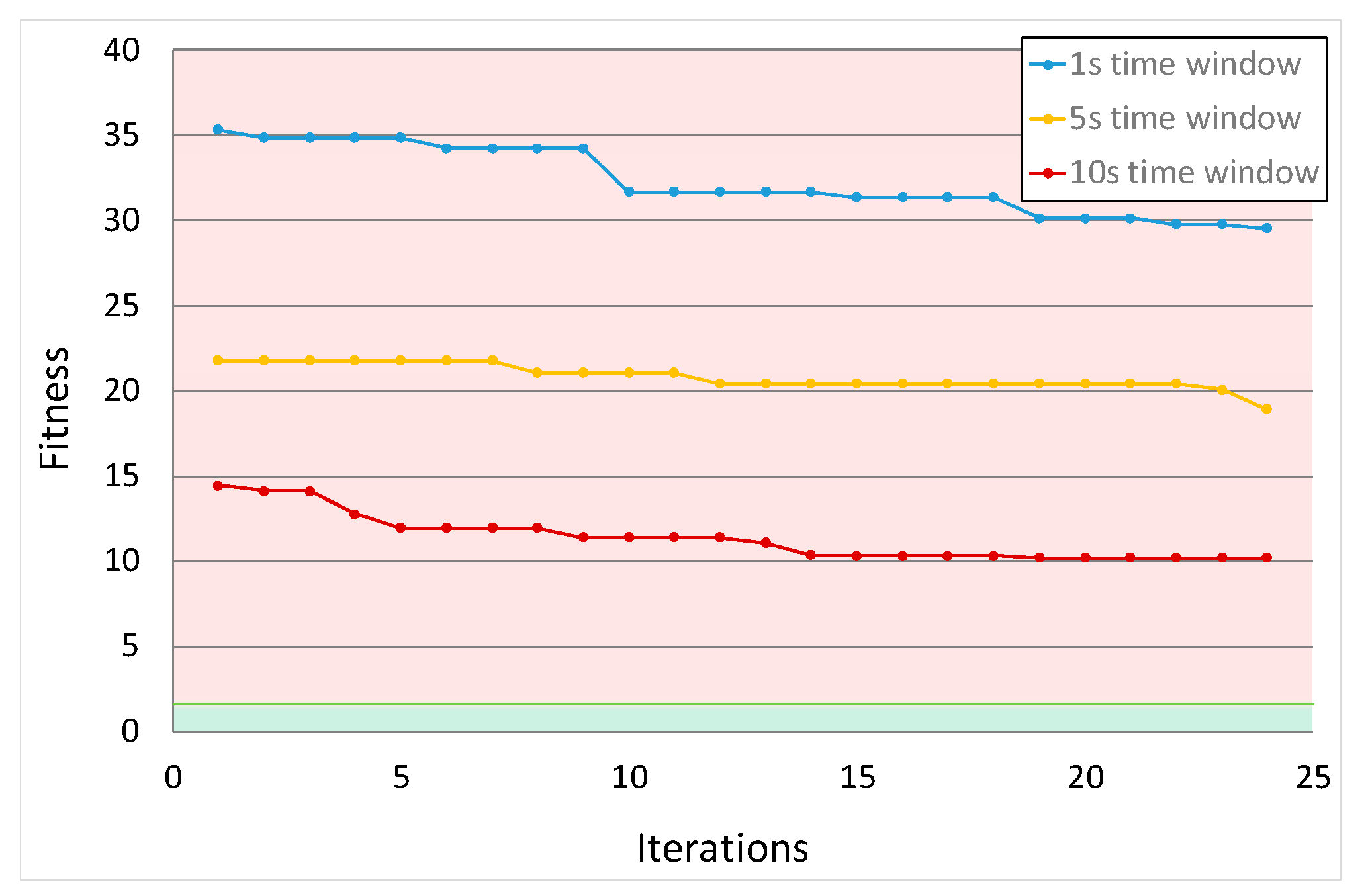
5.1. Benefits of the Proposed Optimisation Method Compared with Single Time Target Approaches

The aim of the optimisation approach proposed in this paper is to find the speed profile with the minimum energy consumption that meets the arrival and the intermediate target times. The typical numerical methods proposed in literature fails when tackle this problem given that they are designed to minimize the energy consumption meeting only the arrival time.

A solution to this problem could be to divide the journey in sections between each pair of target times. However, the solution obtain in each section is not valid for the whole journey. It can be seen in the following example.

A journey with one intermediate timing point is studied. This timing point is located between the departure and the arrival (that is, between 221.3 km and 306.7 km), at position 264 km. The target times chosen for the timing points are taken from the commercial timetable and are listed in

Table 3. Location and target of timing points in the case of one intermediate timing point.

Location of Timing Point	Target Time
264 km	00:12:03
306.7 km	00:26:00

given that the departure time is at 0:00:00.

The journey can be divided in this case in two sections: the first section between the departure station and the intermediate point 264 km (with arrival time of 12 min and 3 s) and the second section between the point 264 km and the arrival point (with arrival time of 26 min).

Each section of the journey is optimised independently and the results are shown in Figure 3. As can be seen, the speed profile of the first section and the speed profile of the second section do not match in their common point 264 km. The speed profile of the first section applies coasting up to 200 km/h when the train approximates to 264 km to save energy. However, the optimisation of the second section starts the train at the maximum speed possible to coast as much as possible and consuming the lowest energy possible.

The previous effect can be neutralized fixing the speed of the train when passing for the 264 km point as can be observed in [65,66]. However, it is needed to choose carefully the passing speed to obtain the minimum energy consumption. It can be observed in the following example.

Figure 4 and

Table 4. Results of the speed profiles obtained for different values of passing speed at 264 km.

Passing Speed (km/h)	Passing Time	Arrival Time	Energy Consumption (MWh)	Difference with Minimum Consumption
300	00:12:03	00:26:00	0.955	0.13 %
235	00:12:03	00:26:00	0.954	0.00 %
200	00:12:03	00:26:00	0.959	0.54 %

show the results obtained optimizing each section of the previous journey independently, fixing the passing speed of the train at 264 km point with different values.

Results indicate that there is a value of passing speed that leads to the minimum energy consumption. Therefore, obtaining the most efficient speed profile dividing the journey would require several levels of optimization to obtain the most efficient passing speeds and the most efficient speed profiles.

On the contrary, the method proposed in this paper solve the problem jointly in a single level, including the intermediate time restrictions in the optimization process. This way, the method proposed is a much more efficient numerical method.

In the following subsections, the results of the proposed method are shown for one and two intermediate target times.

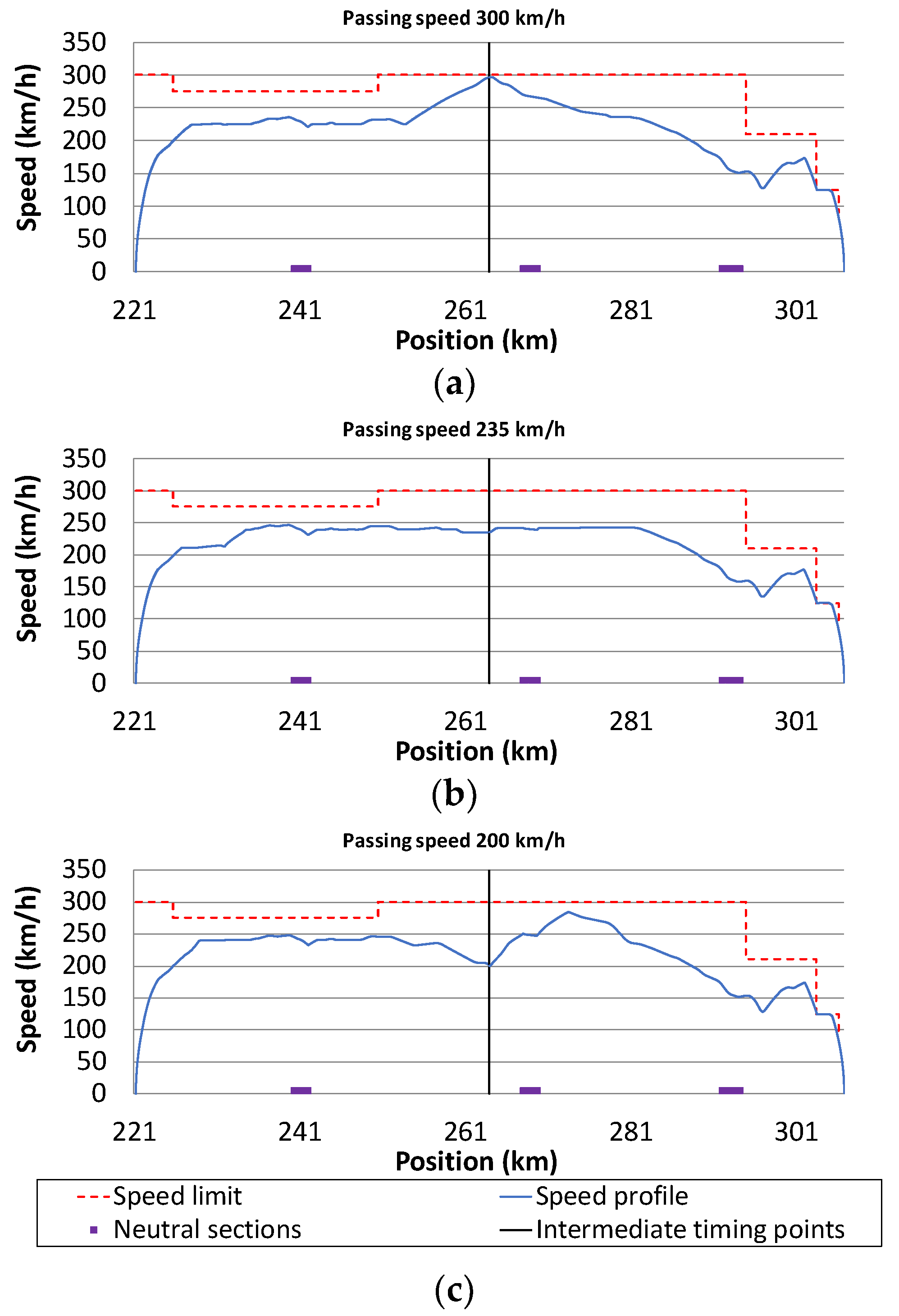
5.2. One Intermediate Timing Point

The case studied is the same journey presented in the previous subsection and defined by the timing points collected in Table 3. Taking into account these restrictions, the algorithms are executed to obtain the speed profile of minimum consumption that fulfils the timing points. Three values for the tolerance have been used to study the influence of the constraint relaxation. These values are 1 s, 5 s, and 10 s.

Figure 5 depicts the evolution of the average value of the 20 tests performed of the fitness of the best solution found by the GA throughout the iterations. In this figure, the three cases of tolerance values are represented.

Furthermore, the area of this figure is divided into two areas by a horizontal line with value located in the position Fitness = 1.52. As explained in Section 4.2, the fitness value of infeasible solutions is the energy consumption of the flat-out driving plus the constrain violation. In this case, the energy consumption of the flat-out driving is equal to 1.52 MWh. Therefore, if the fitness is greater than 1.52, i.e., it is located in the red area, the best solution found by the algorithm at that iteration is infeasible. Contrary, if the fitness is lower than 1.52, i.e., it is located in the green area, the best solution found by the algorithm at that iteration fulfils the timing points restrictions.

As can be observed, the GA is not capable of finding a feasible solution in 24 iterations. The evolution of the algorithm improves the fitness value of the best solution. In other words, the solutions found are closer to the feasible region. However, the fitness improvement between two iterations is too small to find a feasible solution in the iterations given. Comparing the results for the different values of tolerance, it can be seen that solutions found are closer to the feasible region as the tolerance is bigger. Increasing the tolerance gives more flexibility to fulfil the timing points.

On the other hand, the results provided by the DE algorithm present a better performance. Figure 6 shows the evolution of the average value of the 20 tests performed of fitness of the best solution found by the DE at each iteration. The figure is divided into the infeasible red area and the feasible green area as in the previous case.

The results provided by the algorithm has shown its capability to find feasible solutions. In all the 20 tests the algorithm was capable to find a speed profile that meets the target times. As in the case of the GA, the bigger the tolerance, the easier for the algorithm to find a feasible solution. As can be seen in Figure 6, with a tolerance of 1 s the algorithm found a feasible solution at iteration 8, with a tolerance of 5 s the feasible solution is found in iteration 5 and with a tolerance of 10 s the feasible solution is found at iteration 3.

The DE algorithm is capable not only of finding a feasible solution but also of finding an energy efficient solution. Figure 7 shows the same results as in Figure 3, but zooming in the feasible region. This figure shows how the energy consumption of the best solution found by the algorithm is improved during the iterations. Furthermore, these improvements are stabilised at around 15 iterations.

In addition, Figure 7 shows that the energy consumption of the speed profile is lower as bigger is the tolerance. This is mainly because the train can perform higher running time for the whole journey if there is more flexibility (as well at the arrival time). A second order effect is that the more flexibility gives more freedom to perform different speed profiles that can be more efficient.

The energy improvements found by the algorithm are non-trivial. It could be thought that once a speed profile that meets the timing points is found, the rest of feasible solutions will be similar. However, it is possible to obtain a variety of energy consumption results among the feasible speed profiles. For instance, in the case of 1 s of tolerance (which is the most restrictive case), the most energy consuming solution found by the algorithm in all the executions and in all the iterations consumes 1.04 MWh while the most energy efficient solution consumes 0.96 MWh. This is a difference of 7.7%, which is a relevant figure in eco-driving studies.

Figure 8 shows the speed profile of the most efficient and most energy consuming solutions found by the algorithm as well as the timing points. Both solutions meet the target times but in different ways. The most efficient solution presents a smoother speed profile that coasts at 284 km position. On the other hand, the most energy consuming solution reduces its speed just before it has passed the intermediate timing point. This causes that the train must coast later, at 292 km position, to meet the arrival target time. The difference of energy consumption is caused mainly because of the difference in the length of the coasting period performed by the train.

Concerning the computational time, the DE algorithm needs nearly 6 min to complete the 24 iterations demanded. This time is excessive for an online application where the train would need to react to changes in timing points during the journey. However, it is adequate for an offline application where the target times are considered constant.

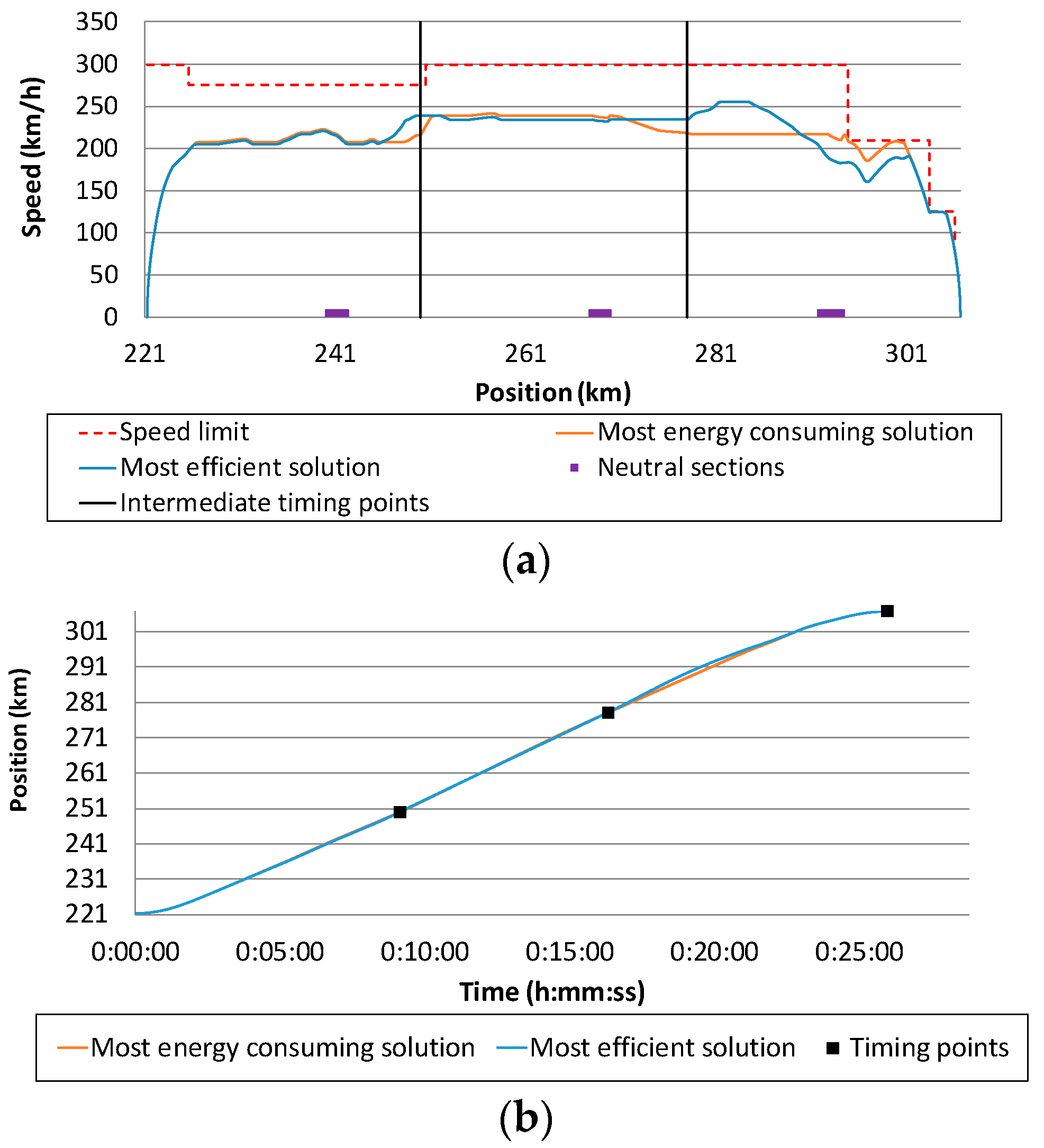
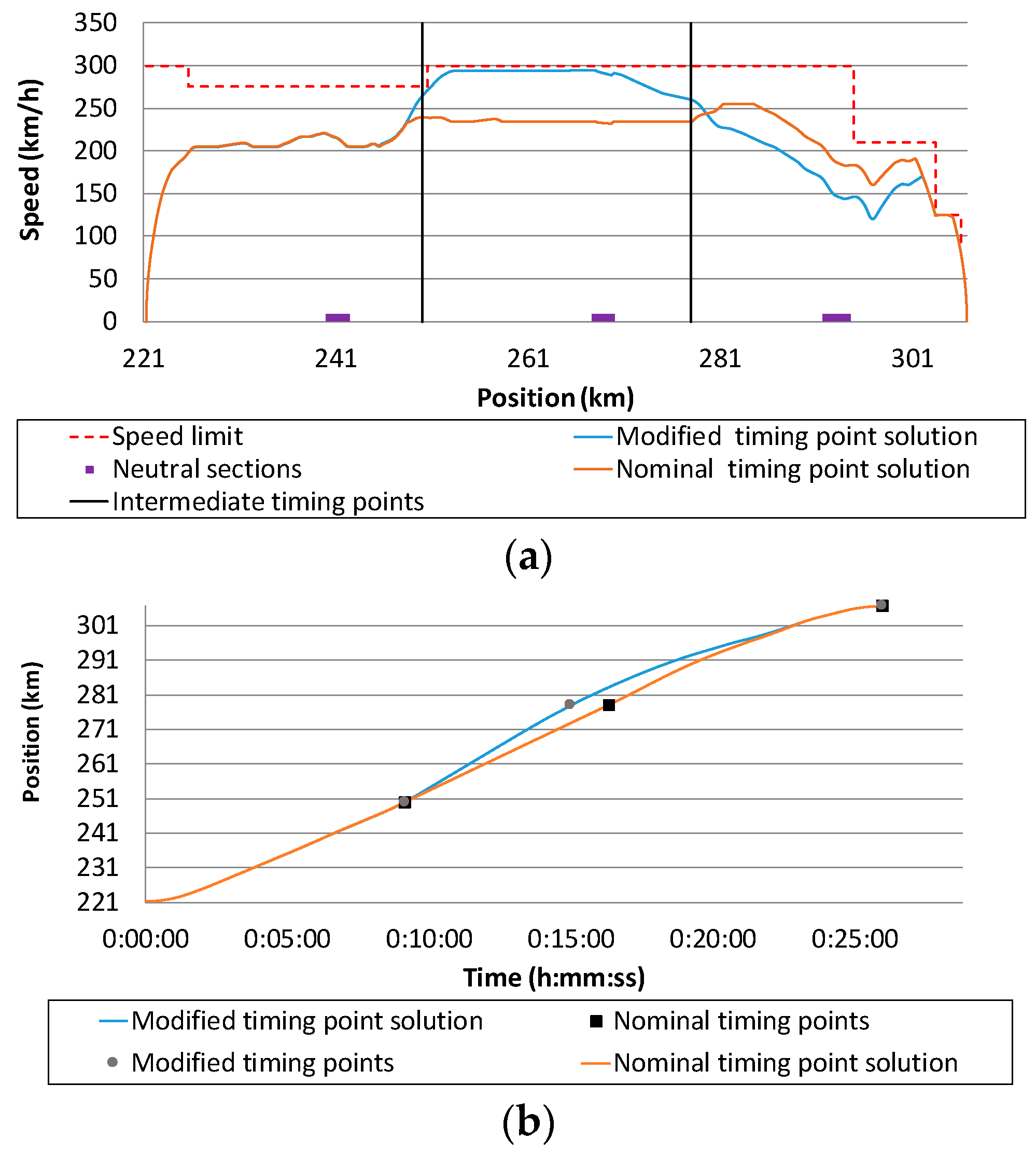
5.3. Two Intermediate Timing Points

In this subsection, the performance of the algorithms in a journey with two intermediate timing points is studied. These points are located at positions 250 km and 278 km. The passing times of the timing points are listed in

Table 5. Location and target of timing points in the case of two intermediate timing points.

Location of Timing Point	Target Time
250 km	00:09:10
278 km	00:16:20
306.7 km	00:26:00

(given that the departure time is at 0:00:00) and, as in the previous example, are based on the commercial timetable.

The DE algorithm and the GA are executed to obtain the speed profile of minimum consumption that fulfils these timing points. As in the previous case, three values for tolerance have been used: 1 s, 5 s, and 10 s.

Figure 9 shows the evolution of the average value of the fitness of the best solution found by the GA throughout the iterations for the three time tolerance values. The figure is divided into the red infeasible area and the green feasible area. As in the previous case, the GA is not capable of finding a feasible solution in 24 iterations.

The DE algorithm is capable of finding feasible solutions although the complexity of the problem has increased with one more restriction. Figure 10 shows the evolution of the mean fitness value of the best solution found by the DE at each iteration.

In all of the 20 executions, the DE algorithm was capable of obtaining a feasible solution. The relaxation of constraints facilitates the search. Figure 10 shows that with a tolerance of 1 s the algorithm found feasible solutions at iteration 10, with a tolerance of 5 s, the feasible solutions are found at iteration 6, and with tolerance of 10 s they are found at iteration 5. Comparing these results with those obtained with one intermediate timing point, it can be seen that, with the new timing point, the algorithm needs more iterations to find feasible solutions. This is because the new restriction reduces the feasible region and it is harder to reach.

Figure 11 is a zoom of the feasible region. It shows that solutions are improved during iterations reducing the energy consumption and it is stabilised before reaching 24 iterations in all the cases. That means that the number of iterations given to the algorithm is enough to converge to the optimal solution. Figure 11 presents, also, the effect of increasing the tolerance.

As in the previous case, it is important to obtain not just a feasible solution, but the best possible one. For instance, in the case of 1 s of time tolerance, the most energy consuming solution found by the algorithm consumes 0.99 MWh, while the most energy efficient solution presents a result of 0.96 MWh. This is a difference of 3.1%, which cannot be neglected. This difference is lower compared to the one obtained in the one intermediate timing point case, because the higher the number of restrictions, the lower flexibility to drive the train and the more similar are the feasible speed profiles.

Figure 12 shows the speed profile of the most efficient and most energy consuming solutions found by the algorithm. Both solutions meet the target times and these two speed profiles are more similar than those shown in the previous section in Figure 8. The main difference between these two solutions is that the efficient speed profile coasts at 285 km position, while the most energy consuming solution does not apply coast, and regulates speed.

The same result in the previous section has been obtained concerning the computational time. The DE algorithm needs nearly 6 min to complete the 24 iterations demanded.

5.4. Effect of the Target Times on the Energy Consumption

It is clear that the arrival timing point has a decisive role in the energy consumed by a train because it determines the running time of the journey. The inverse relationship between the running time and the energy consumption has been widely studied in the literature. Usually, this time is imposed by the timetable so there is no much flexibility to modify it.

On the other hand, intermediate target times can be selected with more flexibility. The intermediate timing points are planned to guarantee the correct crossing order of trains and to ensure the operational separation between trains that run on the same track. Therefore, any intermediate target time can be selected given that the previous criteria are met and the train is capable of fulfilling it.

The intermediate timing points determine the average speed in the different sections of the track. They have an impact on the way the train can be driven and affect directly to the final energy consumption. For this reason, it is necessary to select these target times bearing in mind the effect on the consumption apart from the operational requirements.

The case of one intermediate timing point can be taken to illustrate the effect of the intermediate target time value on the energy consumption. If the intermediate target time is delayed, from the nominal 0:12:03 to 0:14:40, the train will have to perform a different speed profile to meet the new objectives although the arrival target time is maintained. Figure 13 shows the solution obtained by the algorithm with the delayed timing point compared with the solution obtained using the nominal timetable, studied in Section 5.1 and Section 5.2.

It can be seen how the new target time forces slower driving in the first section of the track before the intermediate timing point compared with the nominal timetable solution. In the second section, the new timing point forces the application of flat-out driving. The optimal distribution of the margin time between the first and the second section depends on the slopes of the lane and the speed limitations. In this case, the energy consumption obtained with the new solution is greater (1.14 MWh) than the energy consumption obtained by the nominal timetable speed profile (0.96 MWh). This difference is 18.7% of energy consumption.

Another example can be shown in the case of two intermediate timing points. If the target time of the point located at 278 km is reduced from the nominal timetable 0:16:20 to 0:15:00, the running time available between the two intermediate timing points decreases. As the arrival timing point is not modified, the running time between the second intermediate timing point and the arrival increases. Figure 14 depicts the effect of the modified timing points on the speed profile of the solution obtained by the DE algorithm compared with the nominal solution studied in Section 5.3.

The first section of the journey is very similar for both speed profiles because the first intermediate timing point has not changed. However, the modification of the second target time forces the train to run close to the speed limits until it starts a long coast at 270 km position. This long coast period allows the train to meet the increased time difference between the second timing point and the arrival target. On the other hand, the nominal solution applies a lower holding speed without braking command in the second section and starts to coast at 285 km position. The results show that the modified timing point solution presents higher energy consumption (0.99 MWh) than the nominal speed profile (0.96 MWh). This 3.1% of increase is due to the modifications in the timing points. The energy consumption increases mainly because of the section where the train is driven close to the maximum speed limits. The extra energy consumed during that period is not compensated by the larger coasting period performed later.

These two examples have illustrated that it is important to find the most efficient speed profile given a set of timing points. However, the optimal train operation can only be achieved designing adequately the target times of intermediate timing points. If the timetable associated with intermediate timing points forces the driving to be close to the flat out speed profile, the energy consumption will be higher than if the timing points are designed with energy efficiency criteria. Thus, it is important to design algorithms for the calculation of optimal timetables, to be executed at the track-side equipment of the system.

6. Conclusions

The new ATO over ERTMS system will permit the automatic driving imposing interoperability requirements. In addition, the standard will include energy efficiency requirements for the driving. This paper presents the eco-driving problem defined by the specification of the new system. This eco-driving problem aims to minimise the energy consumption fulfilling the commercial arrival time to the next station. Furthermore, it is subject to new constraints compared with the classical eco-driving problem because of the intermediate target times imposed by the timing points during the journey.

The DE algorithm, a Nature Inspired algorithm, combined with a detailed simulation model, has been proposed to solve this eco-driving problem. This algorithm has been widely applied in the field of constraint optimisation. Besides, a fitness function has been defined to handle the new constraints in the problem. The use of this algorithm makes it possible to find speed profiles that meet the requirements of multiple target times. This is an improvement in numerical eco-driving approaches given that the typical numerical methods proposed in literature cannot be easily adapted to solve this complex problem. The use of a detailed simulation model allows the algorithm to obtain solutions with great accuracy taking into account any detail of the complex railway operation.

The performance of the DE algorithm has been compared with the GA. Both algorithms have been tested in two case studies where one and two intermediate timing points have been taken into account beside the arrival target time. The results have shown that the GA does not find feasible solutions. Contrary, the proposed DE algorithm has demonstrated its capability to find speed profiles that meet all the target times.

Apart from finding feasible solutions, it finds the one with the minimum energy consumption. This task is not trivial since important energy variations have been obtained among feasible solutions. Thus, it has been observed: 7.7% of energy variation in the case of one intermediate timing point and 3.1% in the case of two intermediate timing points. The presence of more constraints reduces the feasible region making more similar the speed profiles that meet all the target times. For this reason, the energy differences observed in the case of two intermediate timing points are smaller compared with the case of one intermediate point.

The time tolerance allowed to meet the target times influences the performance of the algorithm and the energy consumption of the optimal solution. The greater the tolerance the greater the feasible region and the easier to find valid speed profiles. Furthermore, the energy consumption of the solution obtained is lower as greater is the tolerance.

The impact of the target times on the energy consumption has also been shown. Important energy consumption variations have been obtained modifying the nominal timing points. For this reason, the minimum energy consumption on the train operation can be achieved not only obtaining the best speed profile for a given timetable, but also choosing properly the best possible target times (thus, designing an optimal timetable).

The proposed method can be used in real-life applications to forecast the efficient speed profile of train in a journey with intermediate time targets and to offline pre-calculate efficient driving in trains controlled by ATO over ERTMS systems when the timetable is known before the journey.

The execution time required by the algorithm to perform the optimisation is around 6 min. This time is adequate for an offline application. However, this calculation time is excessive to be applied online at the on-board train equipment. In the online application, the timing points can change during the journey, so quick response times are required in the speed profile calculation. For this reason, future work is needed to improve the calculation speed of the algorithm. This future work will be focused on the use of multiple populations in the algorithm, hybridization with other optimization framework, and the use of parallel computing techniques.

References

1. Emery, D. Towards Automatic Train Operation for Long Distance Services: State-of-the Art and Challenges. In Proceedings of the 17th Swiss Transport Research Conference, Ascona, Switzerland, 17–19 May 2017. [Google Scholar]
2. Council of the European Union. Council Directive 96/48/EC of 23 July 1996 on the Interoperability of the Trans-European High-Speed Rail System; European Union: Brussels, Belgium, 1996; pp. 6–24. [Google Scholar]
3. Colla, I.; Consilvio, A.; Olmi, A.; Romano, A.; Sciutto, M. High Density—HD Using ERTMS: The Italian Solution for the Railway Traffic Management. In Proceedings of the 2018 IEEE International Conference on Environment and Electrical Engineering and 2018 IEEE Industrial and Commercial Power Systems Europe (EEEIC/I CPS Europe), Palermo, Italy, 12–15 June 2018; pp. 1–6. [Google Scholar]
4. TEN-T—ATO Project. ATO over ERTMS Operatinal Requirements; European Commission: Brussels, Belgium, 2016. [Google Scholar]
5. ARCC Project. Automated Rail Cargo Consortium: Rail Freight Automation Research Activities to Boost Levels of Quality, Efficiency and Cost Effectiveness in All Areas of Rail Freight Operations; European Commission: Brussels, Belgium, 2020. [Google Scholar]
6. FR8RAIL III. Smart Data for Rail Freight Transport; European Commission: Brussels, Belgium, 2019. [Google Scholar]
7. X2Rail-1. Start-Up Activities for Advanced Signalling and Automation Systems; European Commission: Brussels, Belgium, 2020. [Google Scholar]
8. X2Rail-2. Enhancing Railway Signalling Systems Based on Train Satellite Positioning, On-board Safe Train Integrity, Formal Methods Approach and Standard Interfaces, Enhancing Traffic Management System Functions; European Commission: Brussels, Belgium, 2020. [Google Scholar]
9. X2Rail-3. Advanced Signalling, Automation and Communication System (IP2 and IP5)—Prototyping the future by Means of Capacity Increase, Autonomy and Flexible Communication; European Commission: Brussels, Belgium, 2018. [Google Scholar]
10. X2Rail-4. Advanced Signalling and Automation System—Completion of Activities for Enhanced Automation Systems, Train Integrity, Traffic Management Evolution and Smart Object Controllers; European Commission: Brussels, Belgium, 2019. [Google Scholar]
11. Burton, A.D. Automatic train operation (ATO) specification for Thameslink. Electr. Railw. Lond. Engl. 2001 2009, 54, 188–190. [Google Scholar]
12. Rio Tinto Launches the Autonomous Heavy Freight Rail Operation. Available online: http://sts.hitachirail.com/en/news/rio-tinto-launches-autonomous-heavy-freight-rail-operation (accessed on 26 October 2020).
13. Villalba, M. Pioneering ATO over ETCS Level 2. Railw. Gaz. Int. 2016, 172, 107–109. [Google Scholar]
14. Bienfait, B.; Zoetardt, P.; Barnard, B. Automatic Train Operation: The Mandatory Improvement for ETCS Applications. In Proceedings of the IRSE’s International Technical Conference ASPECT, London, UK, 10–12 September 2012. [Google Scholar]
15. Matsuoka, K.; Kondo, M. Energy Saving Technologies for Railway Traction Motors. IEEJ Trans. Electr. Electron. Eng. 2014, 5, 278–284. [Google Scholar] [CrossRef]
16. Bombardier. Aeroefficient Optimised Train Shaping; Bombardier: Hennigsdorf, Germany, 2010. [Google Scholar]
17. Beusen, B.; Degraeuwe, B.; Debeuf, P. Energy savings in light rail through the optimization of heating and ventilation. Transp. Res. Part Transp. Environ. 2013, 23, 50–54. [Google Scholar] [CrossRef]
18. Das, S.; Abraham, A.; Chakraborty, U.K.; Konar, A. Differential Evolution Using a Neighborhood-Based Mutation Operator. IEEE Trans. Evol. Comput. 2009, 13, 526–553. [Google Scholar] [CrossRef] [Green Version]
19. Li, Z.; Liang, J.J.; He, X.; Shang, Z. Differential evolution with dynamic constraint-handling mechanism. In Proceedings of the IEEE Congress on Evolutionary Computation, Barcelona, 18–23 July 2010; pp. 1–8. [Google Scholar] [CrossRef]
20. Cao, C.; Feng, Z. Optimal capacity allocation under random passenger demands in the high-speed rail network. Eng. Appl. Artif. Intell. 2020, 88, 103363. [Google Scholar] [CrossRef]
21. Abril, M.; Salido, M.A.; Barber, F. Distributed search in railway scheduling problems. Eng. Appl. Artif. Intell. 2008, 21, 744–755. [Google Scholar] [CrossRef] [Green Version]
22. Peña-Alcaraz, M.; Fernandez, A.; Cucala, A.P.; Ramos, A.; Pecharromán, R.R. Optimal underground timetable design based on power flow for maximizing the use of regenerative-braking energy. Proc. Inst. Mech. Eng. Part F J. Rail Rapid Transit 2011, 226, 397–408. [Google Scholar] [CrossRef]
23. Yang, X.; Li, X.; Ning, B.; Tang, T. A Survey on Energy-Efficient Train Operation for Urban Rail Transit. IEEE Trans. Intell. Transp. Syst. 2016, 17, 2–13. [Google Scholar] [CrossRef]
24. Ichikawa, K. Application of Optimization Theory for Bounded State Variable Problems to the Operation of Train. Bull. JSME 1968, 11, 857–865. [Google Scholar] [CrossRef]
25. Howlett, P. Existence of an Optimal Strategy for the Control of a Train; School of Mathematics Report; South Australian Inst. Technol.: Adelaide, SA, Australia, 1987. [Google Scholar]
26. Howlett, P. An optimal strategy for the control of a train. J. Aust. Math. Soc. Ser. B 1990, 31, 454–471. [Google Scholar] [CrossRef] [Green Version]
27. Khmelnitsky, E. On an optimal control problem of train operation. IEEE Trans. Autom. Control 2000, 45, 1257–1266. [Google Scholar] [CrossRef]
28. Liu, R.; Golovitcher, I.M. Energy-efficient operation of rail vehicles. Transp. Res. Part Policy Pract. 2003, 37, 917–932. [Google Scholar] [CrossRef]
29. Howlett, P.G.; Pudney, P.J.; Vu, X. Local energy minimization in optimal train control. Automatica 2009, 45, 2692–2698. [Google Scholar] [CrossRef]
30. Albrecht, A.R.; Howlett, P.G.; Pudney, P.J.; Vu, X. Energy-efficient train control: From local convexity to global optimization and uniqueness. Automatica 2013, 49, 3072–3078. [Google Scholar] [CrossRef]
31. Su, S.; Li, X.; Tang, T.; Gao, Z. A Subway Train Timetable Optimization Approach Based on Energy-Efficient Operation Strategy. IEEE Trans. Intell. Transp. Syst. 2013, 14, 883–893. [Google Scholar] [CrossRef]
32. Miyatake, M.; Matsuda, K. Energy Saving Speed and Charge/Discharge Control of a Railway Vehicle with On-board Energy Storage by Means of an Optimization Model. IEEJ Trans. Electr. Electron. Eng. 2009, 4, 771–778. [Google Scholar] [CrossRef]
33. Miyatake, M.; Ko, H. Optimization of Train Speed Profile for Minimum Energy Consumption. IEEJ Trans. Electr. Electron. Eng. 2010, 5, 263–269. [Google Scholar] [CrossRef]
34. Su, S.; Wang, X.; Cao, Y.; Yin, J. An Energy-Efficient Train Operation Approach by Integrating the Metro Timetabling and Eco-Driving. IEEE Trans. Intell. Transp. Syst. 2020, 21, 4252–4268. [Google Scholar] [CrossRef]
35. Rodrigo, E.; Tapia, S.; Mera, J.; Soler, M. Optimizing Electric Rail Energy Consumption Using the Lagrange Multiplier Technique. J. Transp. Eng. 2013, 139, 321–329. [Google Scholar] [CrossRef]
36. Wang, Y.; De Schutter, B.; van den Boom, T.J.J.; Ning, B. Optimal trajectory planning for trains—A pseudospectral method and a mixed integer linear programming approach. Transp. Res. Part C Emerg. Technol. 2013, 29, 97–114. [Google Scholar] [CrossRef]
37. Wang, Y.; De Schutter, B.; van den Boom, T.J.J.; Ning, B. Optimal trajectory planning for trains under fixed and moving signaling systems using mixed integer linear programming. Control Eng. Pract. 2014, 22, 44–56. [Google Scholar] [CrossRef]
38. Howlett, P.G.; Milroy, I.P.; Pudney, P.J. Energy-efficient train control. Control Eng. Pract. 1994, 2, 193–200. [Google Scholar] [CrossRef]
39. Domínguez, M.; Fernández, A.; Cucala, A.P.; Lukaszewicz, P. Optimal design of metro automatic train operation speed profiles for reducing energy consumption. Proc. Inst. Mech. Eng. Part F J. Rail Rapid Transit 2011, 225, 463–474. [Google Scholar] [CrossRef]
40. Scheepmaker, G.M.; Willeboordse, H.Y.; Hoogenraad, J.H.; Luijt, R.S.; Goverde, R.M.P. Comparing train driving strategies on multiple key performance indicators. J. Rail Transp. Plan. Manag. 2020, 13, 100163. [Google Scholar] [CrossRef]
41. Li, K.; Gao, Z. An improved equation model for the train movement. Simul. Model. Pract. Theory 2007, 15, 1156–1162. [Google Scholar] [CrossRef]
42. Figueira, G.; Almada-Lobo, B. Hybrid simulation–optimization methods: A taxonomy and discussion. Simul. Model. Pract. Theory 2014, 46, 118–134. [Google Scholar] [CrossRef] [Green Version]
43. De Cuadra, F.; Fernandez, A.; de Juan, J.; Herrero, M.A. Energy-Saving Automatic Optimisation of Train Speed Commands Using Direct Search Techniques; Wessex Institute of Technology: Southampton, UK, 1996; Volume 10. [Google Scholar]
44. Zhao, N.; Roberts, C.; Hillmansen, S.; Tian, Z.; Weston, P.; Chen, L. An integrated metro operation optimization to minimize energy consumption. Transp. Res. Part C Emerg. Technol. 2017, 75, 168–182. [Google Scholar] [CrossRef] [Green Version]
45. Tian, Z.; Weston, P.; Zhao, N.; Hillmansen, S.; Roberts, C.; Chen, L. System energy optimisation strategies for metros with regeneration. Transp. Res. Part C Emerg. Technol. 2017, 75, 120–135. [Google Scholar] [CrossRef]
46. Acikbas, S.; Soylemez, M.T. Coasting point optimisation for mass rail transit lines using artificial neural networks and genetic algorithms. IET Electr. Power Appl. 2008, 2, 172–182. [Google Scholar] [CrossRef]
47. Yin, J.; Su, S.; Xun, J.; Tang, T.; Liu, R. Data-driven approaches for modeling train control models: Comparison and case studies. ISA Trans. 2019. [Google Scholar] [CrossRef] [PubMed]
48. Chang, C.S.; Sim, S.S. Optimising train movements through coast control using genetic algorithms. Electr. Power Appl. IEE Proc. 1997, 144, 65–73. [Google Scholar] [CrossRef]
49. Wong, K.K.; Ho, T.K. Coast control for mass rapid transit railways with searching methods. IEE Proc. Electr. Power Appl. 2004, 151, 365–376. [Google Scholar] [CrossRef] [Green Version]
50. Bocharnikov, Y.V.; Tobias, A.M.; Roberts, C. Reduction of Train and Net Energy Consumption Using Genetic Algorithms for Trajectory Optimisation. In Proceedings of the IET Conference on Railway Traction Systems (RTS 2010), Birmingham, UK, 13–15 April 2010; pp. 1–5. [Google Scholar]
51. Lechelle, S.A.; Mouneimne, Z.S. OptiDrive: A Practical Approach for the Calculation of Energy-Optimised Operating Speed Profiles. In Proceedings of the IET Conference on Railway Traction Systems, Birmingham, UK, 13–15 April 2010; p. 23. [Google Scholar]
52. Li, X.; Lo, H.K. An energy-efficient scheduling and speed control approach for metro rail operations. Transp. Res. Part B Methodol. 2014, 64, 73–89. [Google Scholar] [CrossRef]
53. Bocharnikov, Y.V.; Tobias, A.M.; Roberts, C.; Hillmansen, S.; Goodman, C.J. Optimal driving strategy for traction energy saving on DC suburban railways. IET Electr. Power Appl. 2007, 1, 675–682. [Google Scholar] [CrossRef]
54. Cucala, A.P.; Fernández, A.; Sicre, C.; Domínguez, M. Fuzzy optimal schedule of high speed train operation to minimize energy consumption with uncertain delays and driver’s behavioral response. Eng. Appl. Artif. Intell. 2012, 25, 1548–1557. [Google Scholar] [CrossRef]
55. Sicre, C.; Cucala, A.P.; Fernández-Cardador, A. Real time regulation of efficient driving of high speed trains based on a genetic algorithm and a fuzzy model of manual driving. Eng. Appl. Artif. Intell. 2014, 29, 79–92. [Google Scholar] [CrossRef]
56. Lu, S.; Hillmansen, S.; Ho, T.K.; Roberts, C. Single-Train Trajectory Optimization. IEEE Trans. Intell. Transp. Syst. 2013, 14, 743–750. [Google Scholar] [CrossRef]
57. Kim, Y.-G.; Jeon, C.-S.; Kim, S.-W.; Park, T.-W. Operating speed pattern optimization of railway vehicles with differential evolution algorithm. Int. J. Automot. Technol. 2013, 14, 903–911. [Google Scholar] [CrossRef]
58. Ke, B.-R.; Lin, C.-L.; Yang, C.-C. Optimisation of train energy-efficient operation for mass rapid transit systems. IET Intell. Transp. Syst. 2012, 6, 58–66. [Google Scholar] [CrossRef]
59. Xie, T.; Wang, S.; Zhao, X.; Zhang, Q. Optimization of Train Energy-Efficient Operation Using Simulated Annealing Algorithm. In Proceedings of the International Conference on Intelligent Computing for Sustainable Energy and Environment, Shanghai, China, 12–13 September 2012; Li, K., Li, S., Li, D., Niu, Q., Eds.; Springer: Berlin/Heidelberg, Germany, 2013; pp. 351–359, ISBN 978-3-642-37104-2. [Google Scholar]
60. Domínguez, M.; Fernández-Cardador, A.; Cucala, A.P.; Gonsalves, T.; Fernández, A. Multi objective particle swarm optimization algorithm for the design of efficient ATO speed profiles in metro lines. Eng. Appl. Artif. Intell. 2014, 29, 43–53. [Google Scholar] [CrossRef]
61. Fernandez-Rodriguez, A.; Fernandez-Cardador, A.; Cucala, A.P.; Dominguez, M.; Gonsalves, T. Design of Robust and Energy-Efficient ATO Speed Profiles of Metropolitan Lines Considering Train Load Variations and Delays. IEEE Trans. Intell. Transp. Syst. 2015, 16, 2061–2071. [Google Scholar] [CrossRef] [Green Version]
62. Carvajal-Carreño, W.; Cucala, A.P.; Fernández-Cardador, A. Optimal design of energy-efficient ATO CBTC driving for metro lines based on NSGA-II with fuzzy parameters. Eng. Appl. Artif. Intell. 2014, 36, 164–177. [Google Scholar] [CrossRef]
63. Fernández-Rodríguez, A.; Fernández-Cardador, A.; Cucala, A.P. Balancing energy consumption and risk of delay in high speed trains: A three-objective real-time eco-driving algorithm with fuzzy parameters. Transp. Res. Part C Emerg. Technol. 2018, 95, 652–678. [Google Scholar] [CrossRef]
64. Pudney, P.; Howlett, P.G.; Albrecht, A.; Coleman, D.; Vu, X.; Koelewijn, J. Optimal Driving Strategies with Intermediate Timing Points. Ph.D. Thesis, International Heavy Haul Association, Calgary, UK, 2011. [Google Scholar]
65. Albrecht, T.; Binder, A.; Gassel, C. Applications of real-time speed control in rail-bound public transportation systems. IET Intell. Transp. Syst. 2013, 7, 305–314. [Google Scholar] [CrossRef]
66. Quaglietta, E.; Pellegrini, P.; Goverde, R.M.P.; Albrecht, T.; Jaekel, B.; Marlière, G.; Rodriguez, J.; Dollevoet, T.; Ambrogio, B.; Carcasole, D.; et al. The ON-TIME real-time railway traffic management framework: A proof-of-concept using a scalable standardised data communication architecture. Transp. Res. Part C Emerg. Technol. 2016, 63, 23–50. [Google Scholar] [CrossRef]
67. Albrecht, A.R.; Howlett, P.G.; Pudney, P.J.; Vu, X.; Zhou, P. Energy-efficient train control: The two-train separation problem on level track. J. Rail Transp. Plan. Manag. 2015, 5, 163–182. [Google Scholar] [CrossRef]
68. Albrecht, A.; Howlett, P.; Pudney, P.; Vu, X.; Zhou, P. The two-train separation problem on non-level track—Driving strategies that minimize total required tractive energy subject to prescribed section clearance times. Transp. Res. Part B Methodol. 2018, 111, 135–167. [Google Scholar] [CrossRef]
69. Wang, P.; Goverde, R.M.P. Multi-train trajectory optimization for energy efficiency and delay recovery on single-track railway lines. Transp. Res. Part B Methodol. 2017, 105, 340–361. [Google Scholar] [CrossRef]
70. Wang, P.; Goverde, R.M.P. Multiple-phase train trajectory optimization with signalling and operational constraints. Transp. Res. Part C Emerg. Technol. 2016, 69, 255–275. [Google Scholar] [CrossRef]
71. Wang, P.; Goverde, R.M.P. Two-Train Trajectory Optimization with a Green-Wave Policy. Transp. Res. Rec. J. Transp. Res. Board 2016, 2546, 112–120. [Google Scholar] [CrossRef]
72. Coello Coello, C.A. Theoretical and numerical constraint-handling techniques used with evolutionary algorithms: A survey of the state of the art. Comput. Methods Appl. Mech. Eng. 2002, 191, 1245–1287. [Google Scholar] [CrossRef]
73. Mezura-Montes, E.; Coello Coello, C.A. Constraint-handling in nature-inspired numerical optimization: Past, present and future. Swarm Evol. Comput. 2011, 1, 173–194. [Google Scholar] [CrossRef]
74. Baeck, T.; Fogel, D.B.; Michalewicz, Z. Handbook of Evolutionary Computation; CRC Press: Boca Raton, FL, USA, 1997; ISBN 978-1-4200-5038-7. [Google Scholar]
75. Powell, D.; Skolnick, M.M. Using Genetic Algorithms in Engineering Design Optimization with Non-Linear Constraints. In Proceedings of the 5th International Conference on Genetic Algorithms, Urbana-Champaign, IL, USA, 17–21 July 1993; Morgan Kaufmann Publishers Inc.: San Francisco, CA, USA, 1993; pp. 424–431. [Google Scholar]
76. Deb, K. An efficient constraint handling method for genetic algorithms. Comput. Methods Appl. Mech. Eng. 2000, 186, 311–338. [Google Scholar] [CrossRef]
77. Brest, J.; Zumer, V.; Maucec, M.S. Self-Adaptive Differential Evolution Algorithm in Constrained Real-Parameter Optimization. In Proceedings of the 2006 IEEE International Conference on Evolutionary Computation, Vancouver, BC, Canada, 16–21 July 2006; pp. 215–222. [Google Scholar]
78. Zielinski, K.; Laur, R. Constrained Single-Objective Optimization Using Differential Evolution. In Proceedings of the 2006 IEEE International Conference on Evolutionary Computation, Vancouver, BC, Canada, 16–21 July 2006; pp. 223–230. [Google Scholar]
79. Mezura-Montes, E.; Velázquez-Reyes, J.; Coello Coello, C.A. Promising Infeasibility and Multiple Offspring Incorporated to Differential Evolution for Constrained Optimization. In Proceedings of the 7th Annual Conference on Genetic and Evolutionary Computation, Washington, DC, USA, 25–28 June 2005; ACM: New York, NY, USA, 2005; pp. 225–232. [Google Scholar]
80. Kim, D.G.; Husbands, P. Landscape Changes and the Performance of Mapping Based Constraint Handling Methods. In Parallel Problem Solving from Nature—PPSN V; Eiben, A.E., Bäck, T., Schoenauer, M., Schwefel, H.-P., Eds.; Springer: Berlin/Heidelberg, Germany, 1998; pp. 221–229. [Google Scholar]
81. Kim, D.G.; Husbands, P. Mapping Based Constraint Handling for Evolutionary Search; Thurston’s Circle Packing and Grid Generation. In Adaptive Computing in Design and Manufacture; Parmee, I.C., Ed.; Springer: London, UK, 1998; pp. 161–173. [Google Scholar]
82. Sicre, C.; Cucala, A.P.; Fernández, A.; Lukaszewicz, P. Modeling and optimizing energy-efficient manual driving on high-speed lines. IEEJ Trans. Electr. Electron. Eng. 2012, 7, 633–640. [Google Scholar] [CrossRef]
83. Storn, R.; Price, K. Differential Evolution—A Simple and Efficient Heuristic for global Optimization over Continuous Spaces. J. Glob. Optim. 1997, 11, 341–359. [Google Scholar] [CrossRef]
84. Das, S.; Suganthan, P.N. Differential Evolution: A Survey of the State-of-the-Art. IEEE Trans. Evol. Comput. 2011, 15, 4–31. [Google Scholar] [CrossRef]
85. Das, S.; Mullick, S.S.; Suganthan, P.N. Recent advances in differential evolution—An updated survey. Swarm Evol. Comput. 2016, 27, 1–30. [Google Scholar] [CrossRef]
86. Fernández-Rodríguez, A.; Fernández-Cardador, A.; Cucala, A.P. Real time eco-driving of high speed trains by simulation-based dynamic multi-objective optimization. Simul. Model. Pract. Theory 2018, 84, 50–68. [Google Scholar] [CrossRef]
87. Wong, K.K.; Ho, T.K. Dynamic coast control of train movement with genetic algorithm. Intern J. Syst. Sci. 2004, 35, 835–846. [Google Scholar] [CrossRef] [Green Version]
88. Wong, K.K.; Ho, T.K. Coast Control of Train Movement with Genetic Algorithm. In Proceedings of the the 2003 Congress on Evolutionary Computation, CEC ’03, Canberra, Australia, 8–12 December 2003; IEEE: New York, NY, USA, 2003; Volume 2, pp. 1280–1287. [Google Scholar]
89. Yang, L.; Li, K.; Gao, Z.; Li, X. Optimizing trains movement on a railway network. Omega 2012, 40, 619–633. [Google Scholar] [CrossRef]
Figure 1. Optimization method flowchart.
Applsci 10 07705 g001
Figure 2. Track profile, maximum speed limits and neutral zones distribution.
Applsci 10 07705 g002
Figure 3. Speed profile obtained optimizing independently each section between target times.
Applsci 10 07705 g003
Figure 4. Speed profiles obtained optimizing independently each section between target times fixing the passing speed at 264 km to 300 km/h (a), 235 km/h (b) and 200 km/h (c).
Applsci 10 07705 g004
Figure 5. Evolution of the mean value of the fitness of the best solution found by the Genetic Algorithm (GA) for the case of one intermediate timing point.
Applsci 10 07705 g005
Figure 6. Evolution of the mean value of the fitness of the best solution found by the Differential Evolution (DE) algorithm for the case of one intermediate timing point.
Applsci 10 07705 g006
Figure 7. Evolution of the mean value of the fitness of the best solution found by the DE algorithm in the feasible region for the case of one intermediate timing point.
Applsci 10 07705 g007
Figure 8. Speed profile (a) and position evolution with time (b) of the most efficient and most energy consuming solutions found by the algorithm for the case of one intermediate timing point.
Applsci 10 07705 g008
Figure 9. Evolution of the mean value of the fitness of the best solution found by the GA for the case of two intermediate timing points.
Applsci 10 07705 g009
Figure 10. Evolution of the mean value of the fitness of the best solution found by the DE algorithm for the case of two intermediate timing points.
Applsci 10 07705 g010
Figure 11. Evolution of the mean value of the fitness of the best solution found by the DE algorithm in the feasible region for the case of two intermediate timing point.
Applsci 10 07705 g011
Figure 12. Speed profile (a) and position evolution with time (b) of the most efficient and most energy consuming solutions found by the algorithm for the case of two intermediate timing points.
Applsci 10 07705 g012
Figure 13. Speed profile (a) and position evolution with time (b) of the solution found by the algorithm for the case of one intermediate delayed timing point.
Applsci 10 07705 g013
Figure 14. Speed profile (a) and position evolution with time (b) of the solution found by the algorithm for the case of two intermediate timing points with modifications respect to the timetable.
Applsci 10 07705 g014