FEM Modelling of the Influence of the Remaining Windings on the Frequency Response of the Power Transformer

Abstract

One of the standard diagnostic methods for power transformers is frequency response analysis (FRA). This paper deals with progress in the frequency response interpretation of these very important appliances in the power network. Simulations of the frequency response of the transformer windings are a useful way to improve the correct assessment of FRA results. One of the disadvantages of FRA modelling is time-consuming analysis, especially of large multilayer windings. The aim of this article is to develop a numerical model, which would reduce the duration of the electromagnetic field analysis of the winding with hundreds of turns. The approach introduced in the paper describes the simple two-dimensional (2D) finite elements method (FEM) model, which provides the results comparable to the three-dimensional (3D) model. Moreover, the paper presents the numerical models, which demonstrate the influence of the remaining windings on the inductance of tested winding. As a result of the conducted research, the comparison of inductance curve obtained from FRA measurement on the physical model with modelled resonance slope is presented, both for 2D and 3D cases.

1. Introduction

Major failures of transformers have a direct impact on operational ability and reliability of energy supply to consumers, which, when disturbed, leads to an increase in distribution costs [1]. The importance of transformers in the energy system is also affected by the high costs of their repair, especially when it is necessary to remove them from service and the installation site. The most effective way to avoid transformer breakdowns is via their proper maintenance, in particular periodic technical condition assessment. Over the years, several commonly used methods for assessing the technical condition of the power transformers have been developed [2].

Frequency response analysis (FRA) is one of the standard technical condition assessment methods for power transformers. FRA is used to determine the mechanical condition of the active part of the transformer, especially deformations and displacement in the transformer windings, which appear mainly as a result of short circuits and during over-voltages [3]. The FRA method became a standard in 2012, according to IEC 60076-18 [4] and other documents [5,6], which define the principles and techniques of the measurement.

FRA is a comparative method, so it requires the reference measurement (the so-called “fingerprint”) on the same unit performed after construction at the factory or after installation on the worksite in its healthy state. The assessment of the mechanical condition of the measured winding consists, in the interpretation, of the differences between the compared curves. The biggest challenge in interpreting the FRA results is finding the right correlation between curve deviations and damages of the measured winding. Correct analysis of the frequency response (FR) results requires taking into account several factors, including winding geometry, the history of failures, or the connection system. Temperature and moisture content also influence the frequency response of the transformer winding, shifting the FRA spectrum horizontally [7]. Often, the visible changes in two compared curves are not a consequence of deformations in the tested winding, but may come from other components of the transformer [8,9,10]. Consequently, researchers are developing tools, which could help evaluate the FRA test results, including statistical methods [11,12] and methods based on the artificial intelligence [13,14].

One of the possibilities to improve the correct assessment of the FRA results is a simulation of the frequency response. The reason for using the computer models in the assessment of the FRA results is to explain how mechanical faults change the frequency response. In practice, because of high costs of experiments on the real units, the enhancement of a FRA database for the transformers’ active part faults is possible only in the way of numerical simulations (Figure 1) [15].

Recent studies have focused on models that reproduce the FRA signature as close as possible and allow free access to the winding parameters. There are several approaches to establish this goal: mathematical models [16,17], models based on finite element analysis (FEM) [18,19,20], and equivalent electrical circuit models, in particular lumped parameters circuit models [21,22,23,24]. In current FRA research, the lumped parameters circuit models are widely used to examine the behaviour of the FR of the windings.

Although these models combined with the FEM electromagnetic field analysis give satisfactory results, there are many issues that need to be refined in simulations of the FR. One of the problems is the issue of the complexity of multilayer windings with hundreds or thousands of turns. Even small changes in RLC parameters of the tested winding are visible in FRA signature; hence, it is significant to conduct the field analysis as accurately as possible. On the other hand, the three-dimensional (3D) field analysis, taking into consideration the skin-effect in windings, requires very dense meshing. The numerical analysis of such a model is complicated and very time-consuming. The analysis can be simplified by using some approximations, which will allow us to handle the frequency-dependent effects in core material. Another way to increase the FEM analysis efficiency is to develop the two-dimensional (2D) model, what will correspond with the 3D model in high accuracy.

Research carried out in this paper was aimed at developing a winding model that would allow us to determine the inductance of coils as a function of frequency while reducing the duration of the FEM analysis. For this purpose, it was necessary to create both physical and computer models of the coil. To verify the accuracy of the conducted simulations with the measurement on the real coil, the so-called “first resonance”, visible in the FRA spectrum, was used. While obtaining the frequency response for the low voltage (LV) winding, the mutual inductances to the high voltage (HV) windings (even from the other columns), with its bushings and own capacitance, implied the arising of this resonance. This can be seen not only on FRA curves, but also on the frequency dependence of the winding’s inductance. The authors compared the winding inductance obtained via numerical simulations to the inductances received from the FR measurements of the physical coil model. During the simulations, the model based on a real 3D geometry was developed, as well as a simplified 2D model. Because of obvious differences in both models, the process of equalization of the results obtained from the 2D model was undertaken. This process allowed reducing time of the electromagnetic field analysis of the windings with a large number of wires.

2. Frequency Response (FR) Interpretation

During the FRA measurement, the low voltage sinusoidal signal was injected into the one of the transformer terminals in a wide frequency range and measured on the other terminal, with respect to the ground (transformer tank). There were several FRA test configurations; the main was end-to-end open configuration [4], where the signal was applied to the input of the transformer winding and registered at its end. During this measurement, the remaining windings stayed open. This measurement allowed us to examine each winding separately, with some visible impact of the capacitances of the remaining windings [25]. The FRA results were presented as a signal dumping in dB (denoted as FRA) in the frequency domain. A typical spectrum of the FRA amplitude is shown in Figure 2.

Interpretation of the results consists of comparing the differences between the measured curve and the reference curve. As shown in Figure 2, the measurement results can be also compared between phases of the same unit. In these cases, when the damage occurred in one of the windings, the FR of this winding was different from the FR of the other windings. For the aim of the results of interpretation, the FRA spectrum was normally split into three frequency subranges: low (LF range), medium (MF range), and high (HF range). The division made it easier to evaluate the results, because different types of windings deformations affected the behaviour of the FR curve in different frequency ranges.

The shape of the FR curve in the low frequency (LF) range depended mainly on the magnetizing inductance and less on the bulk capacitance of HV-winding. The FR curve in the LF range was sensitive to short circuits between coils and wires. The slope of the curve corresponded to the inductive character of coil impedance in this range. The descending of the curve stopped when the first parallel resonance was reached. After the first resonance, the curve started to increase due to dominant influence of the winding capacitances, and the LF range ended at the inflection point of the curve slope [26].

In end-to-end test configuration on the FR amplitude curve, the first parallel resonance could always be seen. First resonance occurred in the low frequency range and usually had the biggest damping value in the measured FR curve. Generally, the position of the first resonance depends on the winding self-inductance and total capacitance; however, several other factors can influence its position on the FR curve. The position of this resonance on the frequency axis was similar for all coils, despite the fact that there were other types of power transformer windings, which differed in design and number of wires. Resonance phenomenon is associated with the results presented in this paper, because the simulated resonance visible on the frequency-dependent inductance curves had the same background. Research conducted on this subject shows that the position of the first resonance, especially in the FR results for LV windings, depended highly on the mutual inductances and capacitances of the HV windings, even from other phases not directly related to the performed measurement [26,27].

3. Winding models

3.1. Physical Model

The physical model was prepared as a 24-turns coil, wound on the pressboard tube using the rectangular cross-section copper wire and mounted on the outer column of the transformer core. The core originated from the active part of a 800 kVA, 15/0.4 kV, Dy5 distribution transformer, whose dimensions were 961.2 × 1000 mm. As shown in Figure 3, on the other columns of the core, the original transformer windings were mounted. The active part of the transformer was pulled out of the tank and the windings were disconnected from the bushings; hence, they had a small influence on the frequency response of the tested 24-turn coil. However, this influence is crucial for conducted research and is the main problem of this article.

For the physical model, the FRA measurement was carried out in an end-to-end open configuration with an Omicron FRAnalyzer meter in the range from 20 Hz to 2 MHz. On the base of the measured FR of the coil, its frequency-dependent inductance curve was then determined. This inductance curve was used to verify the correctness of the field model of the coil presented below.

3.2. Computer Models

Computer models used for the survey of the analyzed active part of the transformer were created using a software that utilizes the finite elements method (FEM) to compute an electromagnetic field of the model.

The 3D coil model is shown in Figure 4. The model owns the plane of symmetry, so that only half needs to be discretized. At this symmetry plane, the Dirichlet boundary condition was established, so that the magnetic flux could not cross it. The outer boundary of the region took advantage of the “ballooning” condition, therefore the reduction of its volume was possible. The dimensions of the 3D model corresponded to the geometry and dimensions of the physical model. According to this, turns of the coil were evenly distributed along the limb height.

The single wire visible on the outer limb of the core (Figure 4) represented the remaining windings mounted on the core. These windings could be simulated as a one-turn coil, because, during the FRA measurements, they were seen as a concentrated inductance and capacitance. The inductive couplings to other windings, in connection with their capacitances, were clearly visible in the frequency response of measured coil.

The second model used in the research is shown in Figure 5. It was a simplified 2D model, which was prepared utilizing cylindrical symmetry. The outer boundaries of the problem were set as a so-called “ballooning” boundary condition. The analysis in a cylindrical coordinate system caused the model to rotate 360 degrees around the symmetry axis (z axis) during the simulation. Although the final geometry of the 2D model differed from the geometry of the physical and 3D model, it allowed us to perform the field simulation with sufficient accuracy.

Similar to the 3D model, the additional wire located on the right-hand side of the 2D model (Figure 5) represented the other windings mounted on the core. Because of the abovementioned differences between the geometry of 3D and 2D models, the mutual inductance of the analysed coil and the additional wire should take the different value in both cases, so it must be corrected in the 2D model. Therefore, it was necessary to place an additional column in the 2D model, surrounding the additional wire, which allowed us to change this magnetic coupling.

3.3. Electromagnetic Field Calculations

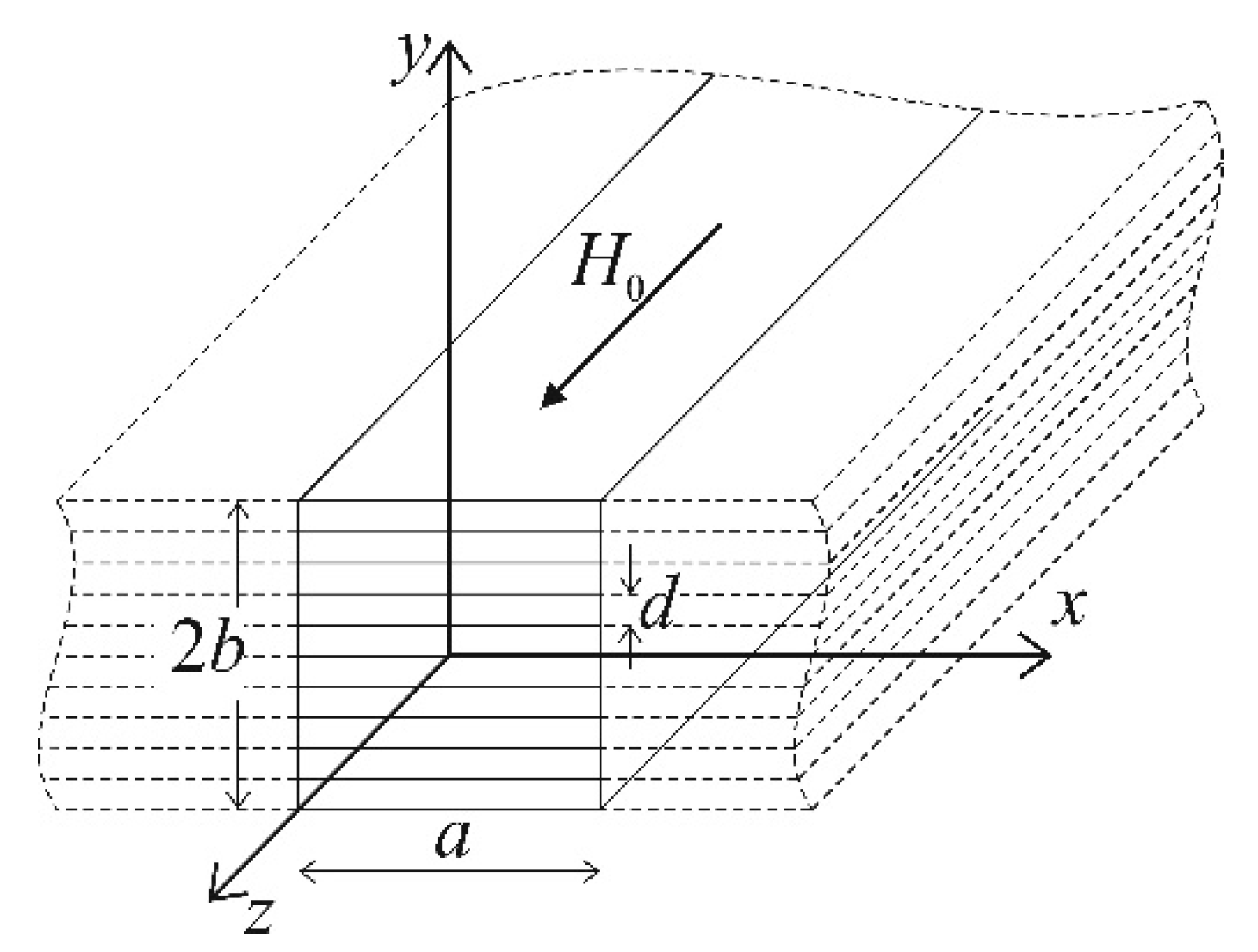
The electromagnetic filed calculations were carried out in ANSYS Maxwell v. 19.2. The software allows to compute the steady-state, time-varying electromagnetic fields in the frequency domain with eddy-current effects. For this aim, the solution of a differential equation for the magnetic vector potential A and the electric scalar potential φ was carried out:

$$\nabla \times \frac{\left(\nabla \times A\right)}{\mu }=\left(\gamma +j\omega \epsilon \right)\left(-j\omega A-\nabla \varphi \right)$$

(1)

where µ is the magnetic permeability, ω is the angular frequency of the source current, γ is the conductivity, and ε is the permittivity.

The self and mutual inductances of the wires were computed on the base of the electromagnetic energy of the field, provided by the FEM:

$$W_{\mathrm{AV}}=\frac{1}{8}{\displaystyle \int B}\cdot H^{\ast }d\mathsf{\Omega }, L=\frac{8W_{\mathrm{AV}}}{I^2{}_{\max }}={\displaystyle \int B\cdot H^{\ast }d\mathsf{\Omega }}$$

(2)

where W_AV denotes the average energy of the magnetic field, L is the winding’s inductance, B is the magnetic flux density, H^* is the magnetic field intensity conjugate, and I_max is the peak value of the excitation current.

ANSYS Maxwell delivered the values of inductances in the form of matrices, which were determined for given frequency, according to the above formulas. For intermediate frequencies, the linear interpolation of inductances was applied.

4. Core Modelling

In order to properly simulate the behaviour of the ferromagnetic core under conditions similar to FRA measurement, in which the input signal was low-voltage and the measurement was made over a wide frequency range, it was necessary to assume the accurate parameters of the core material. Determination of approximate parameters was also necessary to conduct an efficient numerical analysis, taking into account the effect of eddy currents in the winding and core of the transformer [21,28]. The theoretical backgrounds of obtaining the equivalent parameters of the laminated ferromagnetic material, especially an equivalent magnetic permeability and an equivalent conductivity, have been discussed in detail by the authors in previous studies [29] but are shortly presented below, because they are an integral part of the conducted research.

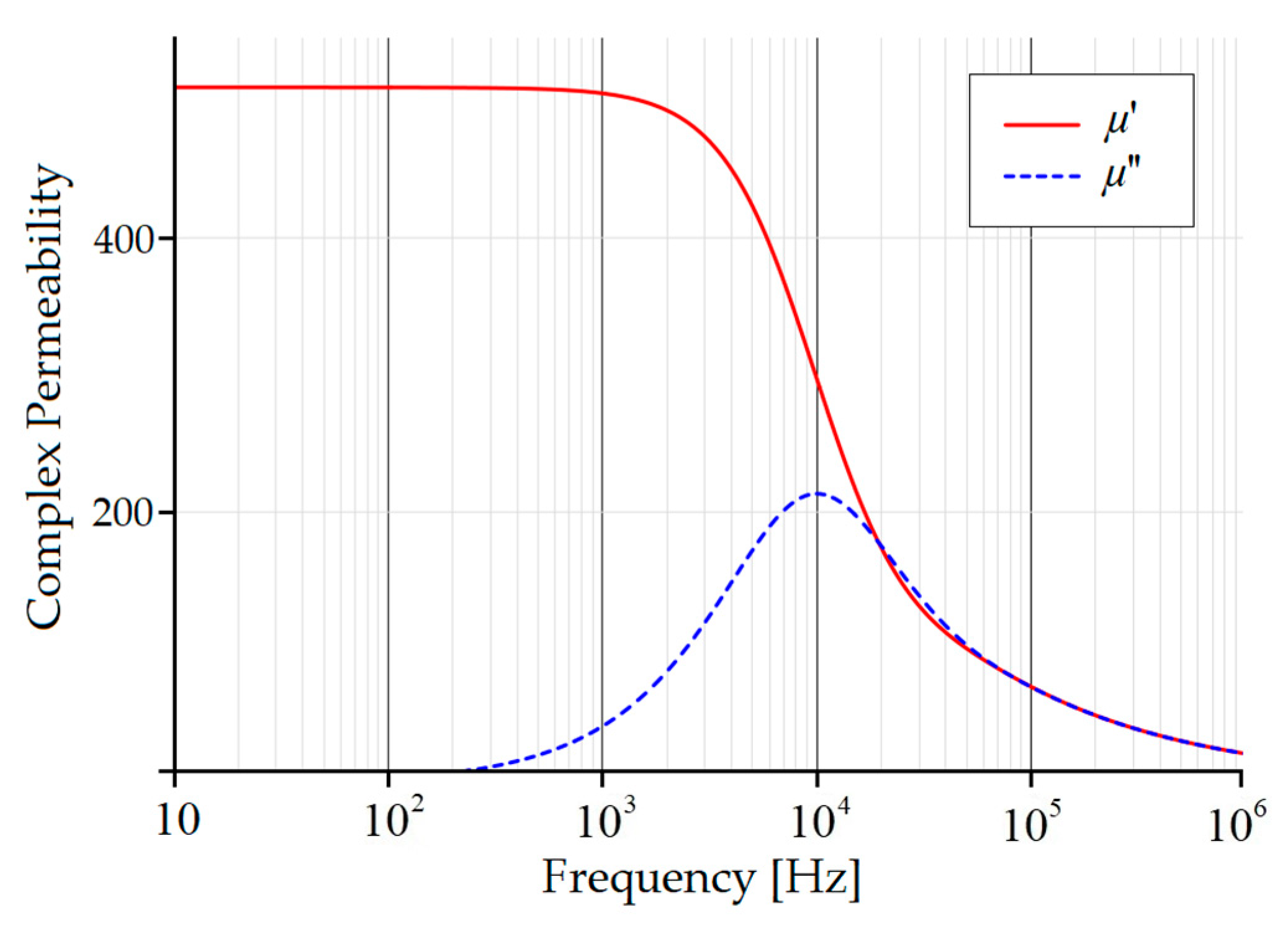
4.1. Equivalent Magnetic Permeability of the Core

For the case of a one-dimensional penetration of the electromagnetic field into the ferromagnetic material, with a thickness of 2D, the only existing y-component of the magnetic intensity vector is given by Formula [30]:

$$H_y(z)=H_{y0}\frac{\cosh kz}{\cosh kD},$$

(3)

where $k=\sqrt{j\omega \mu \gamma }=\frac{\left(1+j\right)}{\delta }$ and $\delta =\sqrt{\frac{2}{\omega \mu \gamma }}$ is the skip-depth.

The complex permeability in the laminated material is defined by Equation [31]:

$$\underset{\_}{\mu }=\frac{1}{H_{y0}}\cdot \overline{B}=\frac{1}{H_{y0}\cdot 2D}{\displaystyle \underset{-D}{\overset{D}{\int }}\left(\mu H_y\right)dz}={\mu }_0{\mu }_{\mathrm{r}}\cdot \frac{\sinh kD}{kD\cdot \cosh kD},$$

(4)

where μ is the complex permeability, μ₀ and μ_r are the vacuum and relative permeability, H_y0 is the magnetic field intensity applied to the surface of lamination, and $\overline{B}$ is the average magnetic flux density.

This complex permeability can by split into real and imaginary parts:

$$\underset{\_}{\mu }={\mu }_0\left(\mu \prime +j\mu ″\right),$$

(5)

$$\mu \prime =\frac{\mathrm{Re}\left(\underset{\_}{\mu }\right)}{{\mu }_0}=\frac{{\mu }_r\delta }{2D}\left(\frac{\sinh \left(\frac{2D}{\delta }\right)+\sin \left(\frac{2D}{\delta }\right)}{\cosh \left(\frac{2D}{\delta }\right)+\cos \left(\frac{2D}{\delta }\right)}\right)$$

(6)

$$\mu ″=\frac{-\mathrm{Im}\left(\underset{\_}{\mu }\right)}{{\mu }_0}=\frac{{\mu }_r\delta }{2D}\left(\frac{\sinh \left(\frac{2D}{\delta }\right)-\sin \left(\frac{2D}{\delta }\right)}{\cosh \left(\frac{2D}{\delta }\right)+\cos \left(\frac{2D}{\delta }\right)}\right)$$

(7)

The real part of the complex permeability corresponds to the conduction of the magnetic flux through the ferromagnetic material, while the imaginary part corresponds to the core loses. The complex permeability as a function of frequency, calculated according to (4), is presented in Figure 6.

In the computer simulation, the values of the real part of the complex permeability were entered separately as input data to the Maxwell software for each simulated frequency.

4.2. Equivalent Conductivity

The equivalent conductivity of the laminated core was used for proper determination of the inductance. The authors decided to use equivalent electromagnetic energy stored in the region of the analysis. As a result, the field analysis may have been reduced to a one-dimensional problem, because, for a single lamination of the core, its thickness d in y direction was much smaller than its dimensions in the other directions. The model of this case is presented in a schematic manner in Figure 7.

The distribution of the z-component of the magnetic intensity vector in the steel sheet of thickness 2b is given by [30]:

$${\underset{\_}{H}}_{\mathrm{z}}=H_0\frac{\cos \mathrm{h}\alpha y}{\cos \mathrm{h}\alpha b},$$

(8)

where ${\alpha }^2=\mathrm{j}\omega \mu {\gamma }_{\mathrm{e}}$ and ${\delta }_{\mathrm{e}}=\sqrt{\frac{2}{\omega \mu {\gamma }_{\mathrm{e}}}}$.

The energy stored in the electromagnetic field is defined by:

$$W_{\mathrm{m}}=\frac{1}{2}\mathrm{Re}{\displaystyle {\int }_{-b}^b\mu \cdot {\underset{\_}{H}}_{\mathrm{z}}\cdot {\underset{\_}{H}}_{\mathrm{z}}^{\ast }\cdot \mathrm{d}y}=\frac{1}{2}{\displaystyle {\int }_{-b}^b\mu \cdot {\left|{\underset{\_}{H}}_{\mathrm{z}}\right|}^2\cdot \mathrm{d}y}$$

(9)

After substituting (8) into (9) and carrying out integration, the energy value is obtained, which corresponds to the equivalent conductivity γ_e of the ferromagnetic block:

$$W_{\mathrm{me}}=\frac{\mu \cdot H_0\cdot {\delta }_{\mathrm{e}}}{4}\frac{\left(\sinh 2\left(\frac{b}{{\delta }_{\mathrm{e}}}\right)+\sin 2\left(\frac{b}{{\delta }_{\mathrm{e}}}\right)\right)}{{\left(\cosh \frac{b}{{\delta }_{\mathrm{e}}}\cos \frac{b}{{\delta }_{\mathrm{e}}}\right)}^2+{\left(\sinh \frac{b}{{\delta }_{\mathrm{e}}}\sin \frac{b}{{\delta }_{\mathrm{e}}}\right)}^2}$$

(10)

The analogue derivation can be made for a laminated core, consisting of n sheets and thickness d and complying with relation 2b = d. Then the energy stored in the laminated core with conductivity γ takes the form of:

$$W_{\mathrm{m}}=\frac{n\cdot \mu \cdot H_0\cdot \delta }{4}\frac{\left(\sinh \left(\frac{d}{\delta }\right)+\sin \left(\frac{d}{\delta }\right)\right)}{{\left(\cosh \frac{d}{2\delta }\cos \frac{d}{2\delta }\right)}^2+{\left(\sinh \frac{d}{2\delta }\sin \frac{d}{2\delta }\right)}^2}\hspace{0.17em}\hspace{0.17em}\hspace{0.17em}\mathrm{with}\hspace{0.17em}\hspace{0.17em}\delta =\sqrt{\frac{2}{\omega \mu \gamma }}$$

(11)

The equality of the W_me and W_m values is accomplished when:

$$\frac{d}{\delta }=\frac{2b}{{\delta }_{\mathrm{e}}}=\frac{n\cdot d}{{\delta }_{\mathrm{e}}},\hspace{0.17em}\hspace{0.17em}\hspace{0.17em}\hspace{0.17em}n\cdot \delta ={\delta }_{\mathrm{e}},\hspace{0.17em}\hspace{0.17em}n\sqrt{\frac{2}{\omega \mu \gamma }}=\sqrt{\frac{2}{\omega \mu {\gamma }_{\mathrm{e}}}}$$

(12)

From (12) follows the relationship for the equivalent conductivity:

$$\hspace{0.17em}\hspace{0.17em}{\gamma }_{\mathrm{e}}=\frac{\gamma }{n^2},$$

(13)

which means that the equivalent conductivity of the laminated core decreases quadratically with the number of laminations in the transformer core.

5. Results

5.1. Equivalent Parameters of Core Material

Simulations of the frequency response require an estimation of the small signal local permeability µ_r, since, during the FRA measurement, excitation of the active part is much smaller than under rated conditions. Usually, the relatively small signal local permeability is about 400–800. In the conducted research, due to the unavailability of the core material sample, this value was determined indirectly by measuring the winding inductance of the physical model, and it was equal to µ_r = 510. The small signal local permeability corresponded with the initial value of the relative permeability and, at higher frequencies values of the permeability, were assumed according to (6) (Figure 6).

Another parameter essential for FEM simulations of the FR is an equivalent conductivity of the core material, which simplifies the model of the laminated core. Equivalent conductivity allows to get around the problem of a highly detailed computational model with very fine finite element mesh by replacing the laminated core with a homogeneous medium with a properly changed conductivity value [32]. The value of isotropic equivalent conductivity can be effectively calculated with (13).

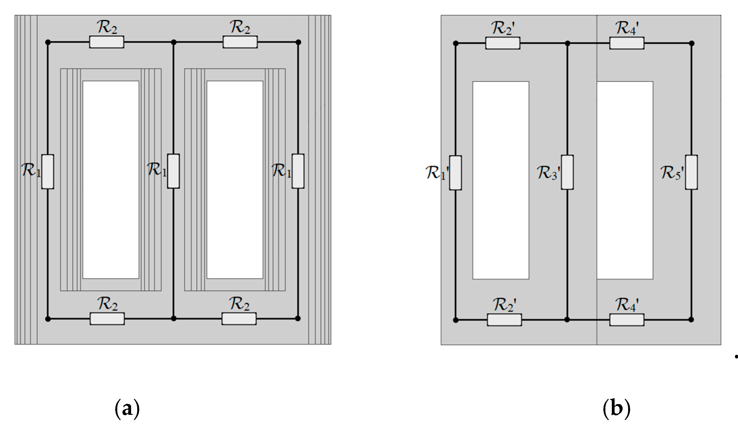
5.2. Equivalence of 2D and 3D Models

The 2D and 3D models were prepared in different coordinate systems, which ultimately lead to differences in the geometry of the obtained objects. While the 3D model strictly corresponded to the geometry of the physical model, the 2D model contained much more ferromagnetic material due to the cylindrical symmetry. Different amounts of the ferromagnetic material in 2D and 3D models caused changes in the value of the reluctance in their magnetic circuits and, as a consequence, in the value of the magnetic flux. The authors assumed that the total magnetic reluctance R in both models were the same. This could be achieved by performing correction of the magnetic permeability in the 2D model. Such an approach is shown in Figure 8 and corresponds to the studies described by Bjerkan [31]. For the considered 2D model, the small signal local permeability was corrected to µ_r = 214, taking into account that the skin depth δ in the 2D model should have the same value as in the 3D model. In both cases, values of the relative permeability at higher frequencies were assumed according to (6).

As mentioned in Section 3 of this paper, the additional column in the 2D model (Figure 5) was used to moderate the value of the magnetic coupling between the analyzed coil and the additional wire. In the 3D model, this magnetic coupling was about 0.3, while in the 2D model, it was 0.14. In order to level up the coupling coefficient in the 2D model, the magnetic permeability value in one of columns was changed. Equalization of the coupling coefficient in the 2D model to the suitable value caused the simulated resonance to arise for the same frequency on the inductance curve.

The main issue of the research was to develop a winding model that would allow us to determine the frequency-dependent inductance of a winding while reducing the duration of the FEM analysis. The resonance visible on the inductance characteristic obtained from the FRA measurements was used to verify the conducted simulations. The resonance occurred above the frequency of 1 kHz (Figure 9) and corresponded to the first parallel resonance visible on the FRA results (this phenomenon was described in detail in Section 2).

The remaining windings, both in the 2D and 3D model, were simulated as the single wire placed on the outer column of the core (Figure 4 and Figure 5), which provided the magnetic coupling with a modelled coil. Since the first resonance depended in particular on the inter-turn capacitances and capacitances to the ground of the other windings, it was necessary to assign the proper capacitance to the additional turn in order to simulate the resonance. In FEM software, this goal is accomplished by creating the output terminal connected to the additional wire with the capacitance C_HV, resulting from the capacitance of the HV-winding. This approach was used both for the 2D and 3D models and is presented in a schematic manner in Figure 5. The value of the capacity of the HV-winding was assumed to be 200 pF; however, because the windings remaining on the transformer core were simulated as a one-turn coil, the value of C_HV had to be recalculated in relation to the single wire. The additional capacitance C_{add_3D} connected to the output terminal in the 3D model is given by:

$$C_{\mathrm{add}\_3\mathrm{D}}=N_{\mathrm{HV}}{}^2\cdot C_{\mathrm{HV}},$$

(14)

where N_HV is the number of turns in the HV-winding, which, for a tested transformer, is equal to 1520. Furthermore, due to the halving of the computational area, C_{add_3D} also had to refer to half of the model. Accordingly, the final additional capacitance C_{add_3D} was equal 240 μF for the 3D model.

The cylindrical geometry in the 2D model caused the diameter of the additional turn to be much larger than in the case of the 3D model; hence, similarly to the case of relative permeability, the value of the additional capacitance for the 2D model had to be corrected. The correction coefficient was related to the value of the inductance of the additional wire in resonance. Since the resonance frequency is known from the FRA measurement and the inductances of the additional wire are known from the FEM simulation, the correlation between the additional capacitance of the 2D and 3D models is given by:

$$\frac{C_{\mathrm{add}\_2\mathrm{D}}}{C_{\mathrm{add}\_3\mathrm{D}}}=\frac{L_{\mathrm{add}\_3\mathrm{D}}}{L_{\mathrm{add}\_2\mathrm{D}}},$$

(15)

where C_{add_2D} is the capacitance of the additional wire in the 2D model, while L_{add_2D} and L_{add_3D} are the inductances of the additional wire in resonance. Accordingly, the final additional capacitance C_{add_2D} of the 2D model was equal 16 μF.

Application of all above principles into the FEM simulation allowed us to obtain corresponding inductance curves for 2D and 3D models. The results of the conducted research are shown in Figure 9, where the inductance characteristic obtained from the FRA measurements was compared to curves determined from the simulations. The resonance was simulated by using the additional capacitance circuits with satisfactory accuracy, both in the 2D and 3D models.

6. Conclusions

At present, the main problem of the FRA method is the reliable interpretation of the obtained results. Due to the high sensitivity of the method, any variation in the values in the RLC circuit of the tested winding causes changes in the FRA spectrum. The modelling of the various mechanical winding’s faults using RLC networks and field models can lead to the development of the fault classification on the basis of FRA and increase serviceableness of this diagnostic method. The presented research shows an approach to the development of a simplified field model, which allows to recreate the inductance of the winding in good accuracy.

When conducting high-frequency modelling of the transformer windings, one should take into consideration that the magnetic field in the ferromagnetic core during the FRA measurements behaves differently than when the transformer is operating under rated conditions. The signal used in FRA measurements is a low-voltage signal, which, in relation to the B–H magnetization curve of the ferromagnetic material of the core, means that, during the FRA measurement, the magnetization of the material is at the beginning of this curve (on its linear section). Furthermore, to handle the eddy-current effects accurately and efficiently, it is necessary to implement the equivalent parameters into the model. The use of the complex relative permeability and the equivalent conductivity cause a significant acceleration of field calculations, as it eliminates a very dense FEM mesh necessary at high frequencies.

The approach presented in the article describes how to create the simple 2D field model, which provides the accurate RLC parameters of the transformer windings. Simplifying the winding model, while not losing accuracy, is important when simulating the frequency response of multilayer windings with a large number of turns, reaching several thousand. Reducing the time-consuming nature of the field analysis can significantly influence the modelling of various mechanical deformations of windings using the lumped parameter circuit models.

The development of a simplified model requires the application of several principles presented in this article. Because of different coordinate systems used for the 2D and 3D analyses, the 2D and 3D models differ in the final model geometry and their parameters. To obtain the equivalent results from 2D and 3D models, the correction factors for the 2D model are presented. The relative permeability, magnetic coupling in the active part, and the additional capacity associated with the windings remaining on the tested transformer should be changed accordingly. As a result of all the above-mentioned principles, the inductance in the wide frequency range of the 2D and 3D FEM models is shown.

References

1. Tenbohlen, S.; Jagers, J.; Bastos, G.; Desai, B.; Diggin, B.; Fuhr, J.; Gebauer, J.; Kruger, M.; Lapworth, J.; Manski, P. Transformer Reliability Survey; Technical Brochure 642 CIGRE: Paris, France, 2015. [Google Scholar]
2. Tenbohlen, S.; Coenen, S.; Djamali, M.; Müller, A.; Samimi, M.H.; Siegel, M. Diagnostic Measurements for Power Transformers. Energies 2016, 9, 347. [Google Scholar] [CrossRef]
3. Senobari, R.K.; Sadeh, J.; Borsi, H. Frequency response analysis (FRA) of transformers as a tool for fault detection and location: A review. Electr. Power Syst. Res. 2018, 155, 172–183. [Google Scholar] [CrossRef]
4. IEC 60076-18: 2012. Power Transformers—Part 18: Measurement of Frequency Response; IEC Standard: Geneve, Switzerland, 2012. [Google Scholar]
5. IEEE Guide for the Application and Interpretation of Frequency Response Analysis for Oil-Immersed Transformers. In IEEE Std C57.149-2012; Institute of Electrical and Electronics Engineers (IEEE): Piscataway, NJ, USA, 2013.
6. Predl, F. Interpretation of Sweep Frequency Response Analysis (SFRA) Measurement Results; OMICRON: Sydney, Australia, 2016. [Google Scholar]
7. Bagheri, M.; Phung, B.; Blackburn, T. Influence of temperature and moisture content on frequency response analysis of transformer winding. IEEE Trans. Dielectr. Electr. Insul. 2014, 21, 1393–1404. [Google Scholar] [CrossRef]
8. Abu-Siada, A.; Hashemnia, N.; Islam, S.; Masoum, M.A. Understanding power transformer frequency response analysis signatures. IEEE Electr. Insul. Mag. 2013, 29, 48–56. [Google Scholar] [CrossRef]
9. Miyazaki, S.; Mizutani, Y.; Tahir, M.; Tenbohlen, S. Influence of employing different measuring systems on measurement repeatability in frequency response analyses of power transformers. IEEE Electr. Insul. Mag. 2019, 35, 27–33. [Google Scholar] [CrossRef]
10. Banaszak, S.; Gawrylczyk, K.; Trela, K.; Bohatyrewicz, P. The Influence of Capacitance and Inductance Changes on Frequency Response of Transformer Windings. Appl. Sci. 2019, 9, 1024. [Google Scholar] [CrossRef] [Green Version]
11. Banaszak, S.; Szoka, W. Transformer Frequency Response Analysis with the Grouped Indices Method in End-to-End and Capacitive Inter-Winding Measurement Configurations. IEEE Trans. Power Deliv. 2020, 35, 571–579. [Google Scholar] [CrossRef]
12. Samimi, M.H.; Tenbohlen, S. FRA interpretation using numerical indices: State-of-the-art. Int. J. Electr. Power Energy Syst. 2017, 89, 115–125. [Google Scholar] [CrossRef]
13. Liu, J.; Zhao, Z.; Tang, C.; Yao, C.; Li, C.; Islam, S. Classifying Transformer Winding Deformation Fault Types and Degrees Using FRA Based on Support Vector Machine. IEEE Access 2019, 7, 112494–112504. [Google Scholar] [CrossRef]
14. Zhao, Z.; Tang, C.; Zhou, Q.; Xu, L.; Gui, Y.; Yao, C. Identification of Power Transformer Winding Mechanical Fault Types Based on Online IFRA by Support Vector Machine. Energies 2017, 10, 2022. [Google Scholar] [CrossRef] [Green Version]
15. Picher, P.; Lapworth, J.; Noonan, T.; Christian, J. Mechanical Condition Assessment of Transformer Windings Using Frequency Response Analysis; Technical Brochure 342 CIGRE: Paris, France, 2008. [Google Scholar]
16. Florkowski, M.; Furgał, J. Modelling of winding failures identification using the frequency response analysis (FRA) method. Electr. Power Syst. Res. 2009, 79, 1069–1075. [Google Scholar] [CrossRef]
17. Wang, S.; Guo, Z.; Zhu, T.; Feng, H.; Wang, S. A New Multi-Conductor Transmission Line Model of Transformer Winding for Frequency Response Analysis Considering the Frequency-Dependent Property of the Lamination Core. Energies 2018, 11, 826. [Google Scholar] [CrossRef] [Green Version]
18. Behjat, V.; Vahedi, A. Numerical modelling of transformers interturn faults and characterising the faulty transformer behaviour under various faults and operating conditions. IET Electr. Power Appl. 2011, 5, 415. [Google Scholar] [CrossRef]
19. Liu, S.; Liu, Y.; Li, H.; Lin, F. Diagnosis of transformer winding faults based on FEM simulation and on-site experiments. IEEE Trans. Dielectr. Electr. Insul. 2016, 23, 3752–3760. [Google Scholar] [CrossRef]
20. Zhang, Z.W.; Tang, W.H.; Ji, T.Y.; Wu, Q.H. Finite-Element Modeling for Analysis of Radial Deformations Within Transformer Windings. IEEE Trans. Power Deliv. 2014, 29, 2297–2305. [Google Scholar] [CrossRef]
21. Bjerkan, E. High Frequency Modeling of Power Transformers, Stress and Diagnostics. Ph.D. Thesis, Norwegian University of Science and Technology, Trondheim, Norway, 25 May 2005. [Google Scholar]
22. Abeywickrama, N.; Serdyuk, Y.; Gubanski, S. High-Frequency Modeling of Power Transformers for Use in Frequency Response Analysis (FRA). IEEE Trans. Power Deliv. 2008, 23, 2042–2049. [Google Scholar] [CrossRef]
23. Gawrylczyk, K.; Banaszak, S. Modeling of frequency response of transformer winding with axial deformations. Arch. Electr. Eng. 2014, 63, 5–17. [Google Scholar] [CrossRef]
24. Abu-Siada, A.; Yao, C.; Abu-Siada, A.; Liao, R. High frequency electric circuit modeling for transformer frequency response analysis studies. Int. J. Electr. Power Energy Syst. 2019, 111, 351–368. [Google Scholar] [CrossRef]
25. Hashemnia, N.; Abu-Siada, A.; Masoum, M.A.S.; Islam, S.M. Characterization of transformer FRA signature under various winding faults. In Proceedings of the 2012 IEEE International Conference on Condition Monitoring and Diagnosis, Bali, Indonesia, 23–27 September 2012; Institute of Electrical and Electronics Engineers (IEEE): Piscataway, NJ, USA, 2012. [Google Scholar]
26. Banaszak, S. Factors influencing the position of the first resonance in the Frequency Response of transformer winding. Int. J. Appl. Electromagn. Mech. 2017, 53, 423–434. [Google Scholar] [CrossRef]
27. Abetti, P.A. Correlation of Forced and Free Oscillations of Coils and Windings. Trans. Am. Inst. Electr. Eng. Part III Power Appar. Syst. 1959, 78, 986–994. [Google Scholar] [CrossRef]
28. Abeywickrama, K.G.N.B.; Daszczynski, T.; Serdyuk, Y.V.; Gubanski, S.M. Determination of Complex Permeability of Silicon Steel for Use in High-Frequency Modeling of Power Transformers. IEEE Trans. Magn. 2008, 44, 438–444. [Google Scholar] [CrossRef]
29. Gawrylczyk, K.; Trela, K. Frequency Response Modeling of Transformer Windings Utilizing the Equivalent Parameters of a Laminated Core. Energies 2019, 12, 2371. [Google Scholar] [CrossRef] [Green Version]
30. Lammeraner, J.; Stafl, M. Eddy Currents; The Chemical Rubber Co. Press: Cleveland, OH, USA, 1966. [Google Scholar]
31. Bjerkan, E.; Høidalen, H.K.; Moreau, O. Importance of a Proper Iron Core Representation in High Frequency Power Transformer Models. In Proceedings of the 14th International Symposium on High Voltage Engineering, Beijing, China, 25–29 August 2005. [Google Scholar]
32. Hahne, P.; Dietz, R.; Rieth, B.; Weiland, T. Determination of anisotropic equivalent conductivity of laminated cores for numerical computation. IEEE Trans. Magn. 1996, 32, 1184–1187. [Google Scholar] [CrossRef]
Figure 1. Diagram of fault detection in the active part of the transformer based on modelling [15].
Applsci 10 07633 g001
Figure 2. Typical frequency response (FR) curves measured on a three-phase transformer.
Applsci 10 07633 g002
Figure 3. Physical model of the 24-turn coil prepared for the conducted research.
Applsci 10 07633 g003
Figure 4. Three-dimensional (3D) model (a) and its discretization into finite element mesh (b).
Applsci 10 07633 g004
Figure 5. Two-dimensional (2D) coil model with additional circuit (a) and its discretization into finite element mesh (b).
Applsci 10 07633 g005
Figure 6. Complex permeability as a function of frequency (2D = 0.23 mm, µr = 510, γ = 1.2·106 S/m).
Applsci 10 07633 g006
Figure 7. A model of a laminated core with infinite x, z dimensions.
Applsci 10 07633 g007
Figure 8. The reluctance network of the 3D model (a) and 2D model (b).
Applsci 10 07633 g008
Figure 9. The inductance of the tested coil as a function of frequency. 2D and 3D finite elements method (FEM) models compared with the inductance obtained from frequency response analysis (FRA) measurements.
Applsci 10 07633 g009
Publisher’s Note: MDPI stays neutral with regard to jurisdictional claims in published maps and institutional affiliations.