Abstract
To quantify the annual probability of earthquake ground motion (GM) exceeding a given threshold, the extensively used method named by probabilistic seismic hazard analysis (PSHA) can be adopted. The PSHA software made this method more effortless for estimating earthquake hazards for a seismic site. The main motivation of the PSHRisk-tool is to evaluate the PSHA by a user-friendly graphical interface as well as identify the intensities of GM, which will contribute to the most vulnerable condition for the infrastructure. This python-code based tool can demonstrate the source identification, probability distribution plot of magnitude and distance, formulate the hazard curve according to almost all ground motion prediction equations (GMPEs). The deaggregation for each intensity measure (IM) and the effect of seismic parameters in each GMPE can also be determined. Alongside this, the combination of the failure frequency and the hazard analysis for identifying risk assessment separates this tool from the other existing PSHA software. Accurate verification with analytical and existing test models and a case study inspires its acceptance rate. However, with the quickest and easiest way users can determine the seismic hazard analysis for any location. Failure risk analysis can be evaluated simply based on the structural failure parameters.
1. Introduction
To address the structural safety against earthquakes, the seismic risk analysis first consists of determining the annual probability of exceeding a certain level of ground motion at a site [1,2]. This level of an earthquake depends on several uncertainties, where the seismic risk uncertainties are related to the location, size, frequency, and effect of an earthquake. Therefore, the probabilistic seismic hazard analysis (PSHA) combines those probable uncertainties to generate a clear description of the distribution of future site seismic excitation. In order to know the ground motion (GM) characteristics, the PSHA method has a defendable power for predicting the potential shaking intensity by future earthquakes. Taking advantage of the seismic models in any seismically induced site, this method explains how local information can be used to define the uncertainty in earthquake magnitude and peak ground acceleration (PGA).
Simultaneously, in the case of structural seismic response, the identification of the most contributing intensity measure (IM) for failure risk can be measured by the concept of mean annual frequency of failure as used by Eads et al. [3,4] which is the combination of the seismic hazard and the structure’s failure probability. After taking the GM based on the structural site seismic hazard analysis, the failure probability is determined by the fragility analysis [5]. Therefore, the deaggregation of the mean annual frequency of failure risk in terms of PGA (IM) can be evaluated for identifying which intensities contribute most to the structural collapse risk in the case of different damage stages.
This study will introduce details about the PSHRisk-tool that can show the PSHA for a site and as well as the failure risk assessment of the structural response. PSHRisk-tool is scripted by the Python programming language, because it is an interpreted, high-level, general-purpose, comparatively simple to learn, and platform-independent, and enables the development of interactive GUI. Until now, many tools have been developed that can calculate PSHA. FRISK88M (v1.8) is one of them that can determine the probabilistic seismic hazard assessment, written in FORTRAN language [6]. This software follows the classical PSHA method and also includes earthquake recurrence models and seismic source models. Scripted in Java language, the software OpenSHA can be considered more a library of Java classes than a rigid PSHA code. This software can estimate the exceedance probability as a function of the intensity measure level by considering the potential influence of all ruptures in the Earthquake Rupture Forecast (ERF) at the site [7,8]. In addition, EQRM is a Python-based software developed for Geoscience Australia’s Earthquake Risk Model, which can calculate the event-based earthquake scenario and scenario loss modeling as well as a probabilistic seismic hazard (PSHA) and risk (PSRA) modeling [9]. Besides these, there is other software packages such as SeisHAZ, MoCaHAZ, MRS, OHAZ, SESIRISK IIIM, REASSESS V2.0, which are created by different languages and have been used in several projects all around the world. Some of them have limited GMPE models and some of them lack a user-friendly GUI and nowadays software needs to be expressed in a graphical representation along with long command lines and compact stand-alone package files.
Similar to the previous PSHA software, the PSHRisk-tool also can provide a seismic hazard analysis of any source by just providing the “latitude” and “longitude” or as a coordinate value of a specified site. By using this software one can estimate the probability of distance distribution between the earthquake source and the specified site considering four different sources, i.e point, line, area and 3D faults. For magnitude-frequency distribution, it follows the exponential magnitude distribution model proposed by Youngs and Coppersmith [10] and the probability density function of earthquake magnitude of Pailoplee and Palasri [11]. This tool supports the earthquake hazard determination for 21 attenuation models by default and these are taken from Abrahamson and Silva [12], Abrahamson and Silva [13], Ambraseys [14], Ambraseys [15], Boore et al. [16], Campbell [17], Campbell [18], Campbell [19], Campbell and Bozorgnia [20], Campbell and Bozorgnia [21], Cornell et al. [22], Donovan [23], Faccioli [24], Faccioli [25], Joyner and Boore [26], Joyner and Boore [27], McGuire [28], Orphal and Lahoud [29], Sadigh et al. [30], Zare and Sabzali [31], Laouami [32], Podili and Raghukanth [33] and Bajaj and Anbazhagan [34]. There are more than 500 attenuation models in the past literature [35]. One of the prime advantages of this tool is the users can implement any attenuation model without difficulty.
In addition to these features, another addition of this tool articulated in this study is the failure risk assessment (FR-assessment) of any infrastructure. Failure risk is measured via the mean annual frequency of collapse (), which combines the seismic hazard and the probability of failure of structures conditioned on GM intensity [36]. The extension of the PSHA curve as named by the deaggregation plot for a specific IM can be computed to know the largest contribution to the hazard. For mitigating the uncertainties in GM, the target earthquake level can also be obtained through PSHA analysis. For the failure risk assessment, the fragility parameters (mean and standard deviation) need to be input for the failure intensity measure of each GM. This assessment can be done for different performance levels or different damage states. Analytical result verification using existing well-known software makes the PSHRisk-tool more acceptable. The efficiency has been textualized through the case study for the Korean Peninsula. This tool can be specialized from both the IT perspective and a seismic hazard as well as failure risk perspective. The source code is available on request, is fully portable (platform-independent) for the user and capable of high-range computations as well. Therefore, the authors believe that although the features of this first version may look similar to the general aspects of other PSHA software, the incorporation of the structural failure risk assessment makes it different from others.
2. Theoretical Supports
PSHA is a classical method to estimate the hazardous earthquake shaking for a specific site. This method deals with all possible uncertainties related to the earthquake magnitude, location, resulting in shaking intensity and the variation of GM characteristics with earthquake size and location [1,11,37].
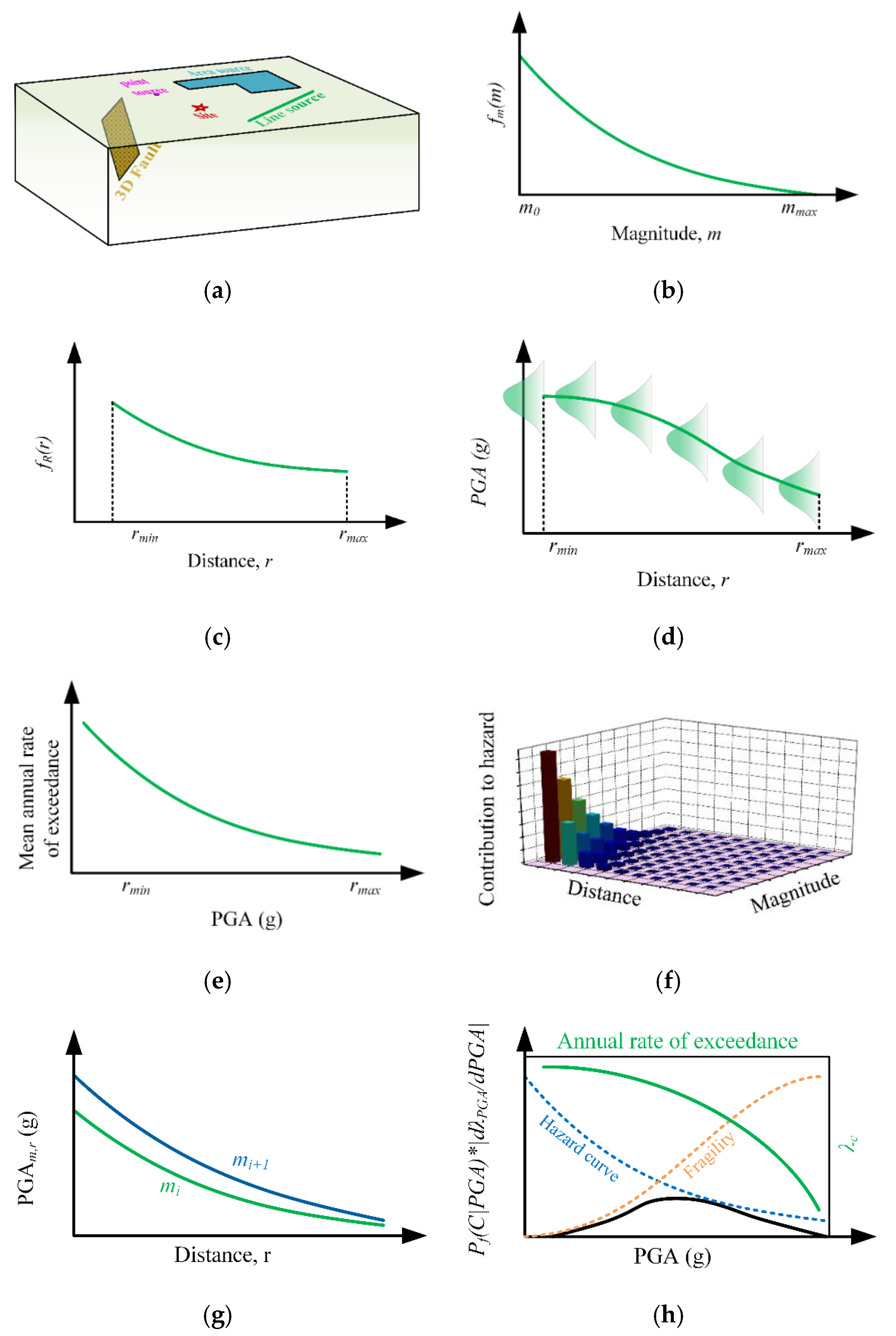
Therefore, the PSHA methodology is associated with the mathematical models of the size and location of potential future earthquakes. With the help of these backgrounds, the PSHRisk-tool performs the following tasks as shown in Figure 1, which are divided into four parts (PSHA, EPSHA, GMPE and FR_Assessment) in this tool.

Figure 1.
Schematic illustration of the basic steps for the analysis by PSHRisk-tool: (a) Earthquake sources identification, (b) Earthquake magnitudes distribution from each source, (c) Distribution of source-to-site distances, (d) Attenuation relation, (e) Combination of parts a-d to compute the seismic hazard curve, (f) EPSHA analysis, (g) GMPE plotting for specific source-site, (h) Failure risk assessment.
2.1. Source Identification and Source-to-Site Distribution
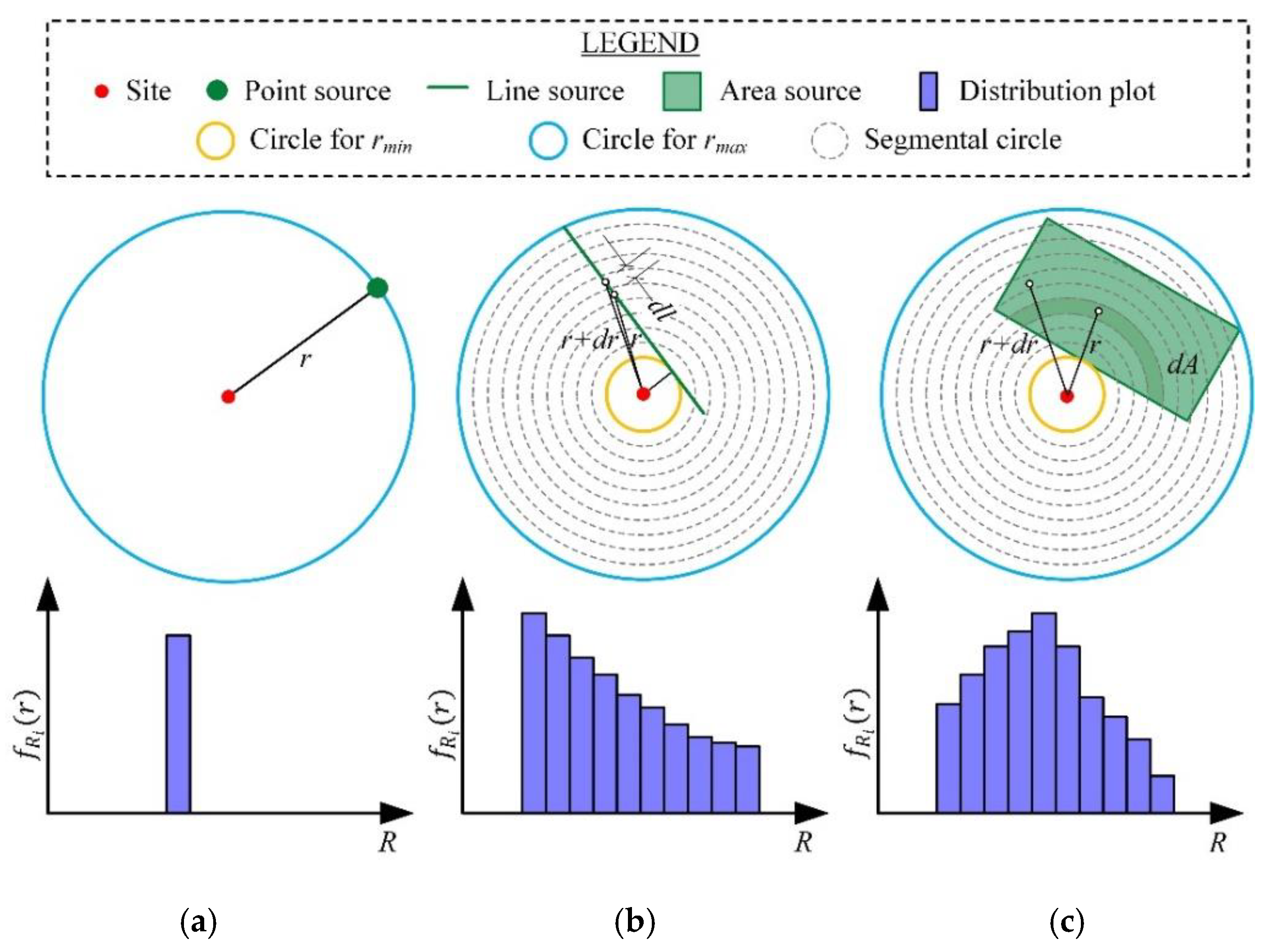
To characterize the earthquake source and to predict ground shaking at a site (the location where one is interested in knowing the seismic hazard or risk), it is important to consider the geometry. The source has been classified according to the formulation of an earthquake fault. Depending on the geometry of any source like point source, line source, area source, grid source, rectangular fault, etc., the distance can be taken as epicentral distance, hypocentral distance, Joyner and Boore distance and closest distance to the fault rupture. The probability of source distribution can be done by a probability density function (PDF) or cumulative distribution function (CDF) throughout a particular source zone. Generally, three kinds of source-to-site distance distribution are illustrated by the mathematical explanation in Kramer [37], Cornell [2] and Baker [1] as shown in Figure 2.

Figure 2.
Examples of source-to-site distance for different source geometries and probability distribution: (a) Point source, (b) Line source, (c) Area source.
In the case of a point source, if the distance of the source-to-site distance is , the distribution probability for is assumed to be one and the probability for is zero. For the linear source, the fault between and is equal to the probability that occurs between the and by the following equation:
where and are the CDF for the variables of and respectively.
And if the earthquakes are needed to distribute uniformly over the length of the fault, when the CDF for will be:
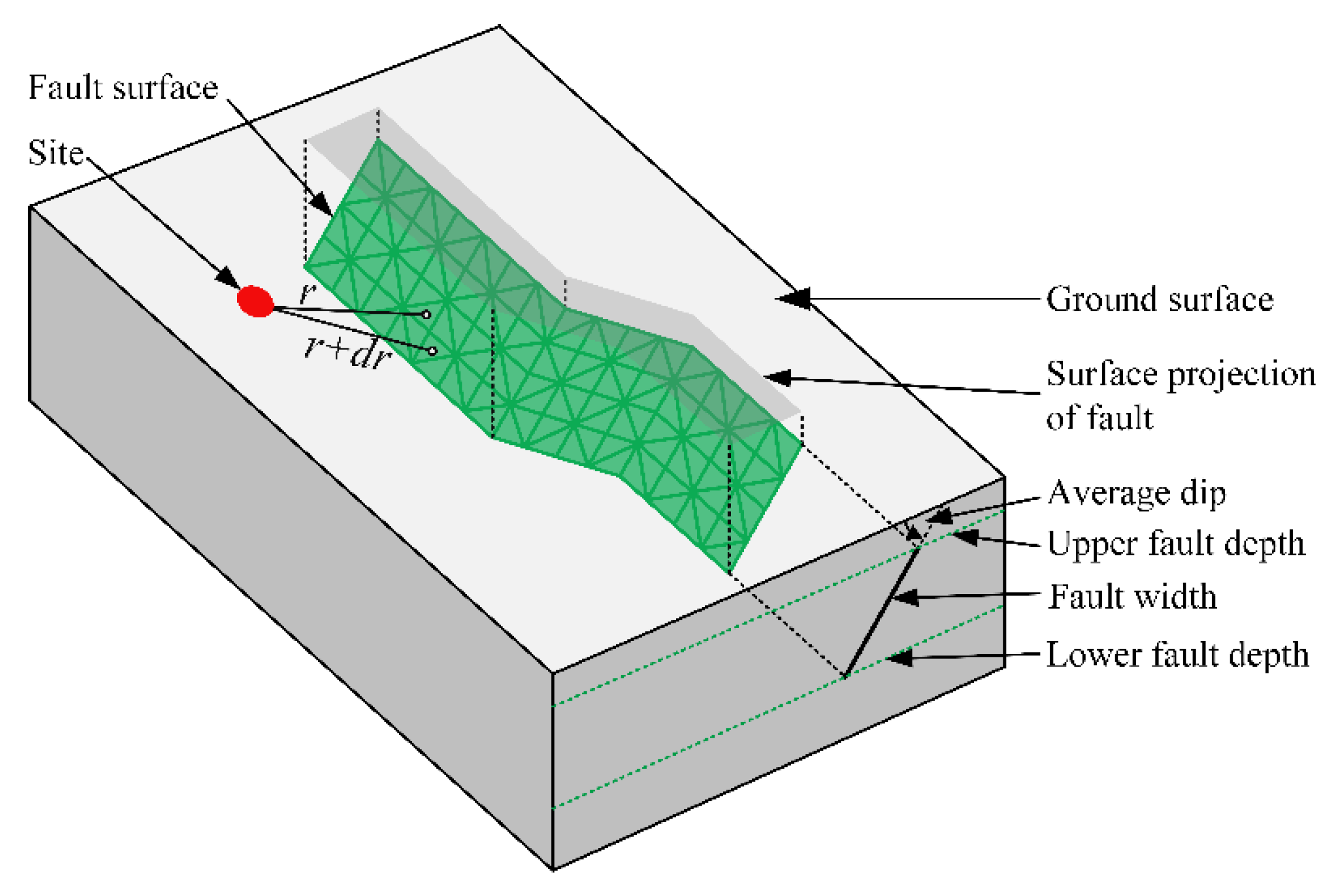
For the area source, the distribution is also followed similarly to the linear source. PSHRisk-tool first converts the geographic coordinates of latitude-longitude into the corresponding Cartesian coordinates (if needed) with site location. In the case of a 3D fault, triangular meshing is used for the discretization of faults (Figure 3). The triangular meshing is more advantageous for modeling a curved fault as there is no overlap between adjacent elements. The triangular element size on the fault can be modified to satisfy the grid resolution requirements.
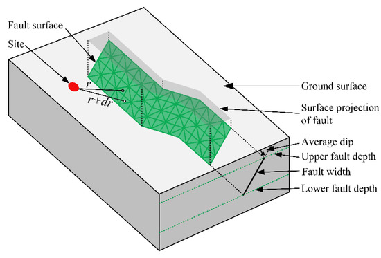
Figure 3.
3D fault source discretization.
2.2. Uncertainty and PDF of Earthquake Magnitude
After identifying the earthquake source and characterizing the corresponding source zone, it is necessary to turn towards the expected sizes (i.e., magnitudes) of the earthquake that the source zone can be expected to produce. Each source produces different sizes of an earthquake up to the maximum earthquake and smaller earthquakes occur more frequently than larger ones. This uncertainty can be solved by the distribution of the earthquake sizes in a given period of time with a well-established recurrence law. Usually, the probability density function for a given size of an earthquake followed the Gutenberg and Richter [38] recurrence law, which is expressed as:
where indicates the annual rate of exceedance of magnitude m, a, and b; values are known as the Gutenberg-Richter recurrence parameters, . If the earthquakes are greater than the threshold magnitude , the mean annual rate of exceedance can be explained [39] as follows:
where .
According to the Youngs and Coppersmith [10], the CDF and PDF for Gutenberg and Richter [38] law with the possible maximum () and minimum () magnitudes can be expressed [37] as:
Therefore, the seismicity parameters a, b, , of each source, the model is a pivotal part of probabilistic seismic hazard analysis. Youngs and Coppersmith [10] gave an equation for the annual rate of earthquake occurrence for the exponential magnitude distribution model by the following expression:
where µ is the shear modulus, is the rupture area, is the slip rate, is the seismic moment for [11].
In the case of only one magnitude value (m), the seismic moment rate (the number of earthquakes of magnitude equal to m in one year) can be expressed as:
where shear modulus, A = source area (km2) and s = average slip rate on the fault (cm/year).
2.3. Probabilistic Seismic Hazard Analysis (PSHA)
PSHA accounts for all surrounding potential seismic sources to quantify seismic hazard at a site by and consider all possible aleatory uncertainties (magnitudes , distances and epsilons ), which affects the GMs The PSHA integrals the combination of these parameters to compute the total exceedance rate [1,11,37] of a given IM can be expressed by the following equation:
where is the rate of occurrence of earthquakes greater than and is the rate of are the probability density functions for the earthquake magnitude and the distance from the earthquake source to the site, respectively. ) is the probability of under a condition for an earthquake event of magnitude m occurred at source-to-site distance , which results from a GMPE or attenuation equations.
The rate of exceedance of a specific value of ground shaking of the earthquake can be estimated by the PSHA approach. According to the process of PSHA described by Kramer [37] and Baker [1], the probabilities distance or magnitude distribution varies in among multiple GMs with a common earthquake magnitude and distance . This can be introduced as the number of standard deviations by which a given logarithmic spectral acceleration differs from the predicted mean logarithmic spectral acceleration, as shown in mathematical form in the following equation [40]:
where is the standard normal distribution function and here for example is the mean log peak ground acceleration (in units of ) proposed by Cornell et al. [22] and Baker and Allin Cornell [41].
2.4. GMPE Parameters
The ground motion prediction model is generally developed using statistical regression of observed ground motion intensities. The GMPE models are capable to give a PDF of ground motion, showing the relation with different GMPE parameters like rupture distance, magnitude, fault type, site conditions, etc. [1]. Ground Motion Prediction Equations (GMPEs) are sometimes referred to as attenuation models. Twenty-one GMPE models have been taken to quantify this tool, where these models differ with distance. All of them are listed in Table 1.

Table 1.
Variation of GMPE parameters.
2.5. Extended Probabilistic Seismic Hazard Analysis (EPSHA)
The PSHA is a method of seismic hazard analysis which aggregates all the possible sources in one platform. Nevertheless, this aggregation may cause sometimes difficulties in understanding which earthquake is most likely to cause [1]. Therefore, the process of removing the terms of summations in the Equation (10) is known by the phenomenon of EPSHA or deaggregation [43,44]. The deaggregation can be defined as the mean annual rate of exceedance for particular ground motion intensity as a function of magnitude or as a function of source-to-site distance or as a function of both by the following equations:
or:
or:
Therefore, for the contribution of each GMPE to its corresponding ground motion parameters, the deaggregation can be mathematically written by as follows:
where is the return period and by using the given IM (PGA), one can get a return period indirectly from the hazard curve.
2.6. Failure Risk Assessment (FR-Assessment)
The failure risk quantification of a structure can be possible by the concept of failure risk assessment. This can be measured via the mean annual of failure () (either as a limit state or performance-based), which is the combination of the structural failure probability analysis for different failure states and the seismic hazard analysis [3].
The structural failure probability is defined as the probability of failure, that the seismic demand placed on the structure is greater than the capacity of the structure [45]. In another word, the fragility curves are defined as the seismic capacity of mechanical and structural systems in the form of a probability distribution function, usually as a function of the intensity measures such as peak ground acceleration, spectral acceleration, peak ground velocity, spectral intensity, spectral velocity, etc. [46]. The GM of IM is scaled by the IDA method, where according to Ibarra and Krawinkler [5], the fragility curve is calculated from data sets by taking logarithms of each GM’s value corresponding to the onset of the collapse. Equations (16) and (17) show the mean and standard deviation of the fragility curve:
where n is the number of considered GMs and is the value associated with the onset of collapse for the th GM. The mathematical explanation of PSHA has been done previously and the failure risk assessment curve can be explained by the combination of fragility function and PSHA function as follows:
where is the failure probability of the structure, the ground motion intensity is indicated by IM and is the slope of the seismic hazard curve [3,36].
3. Application of PSHRisk-Tool
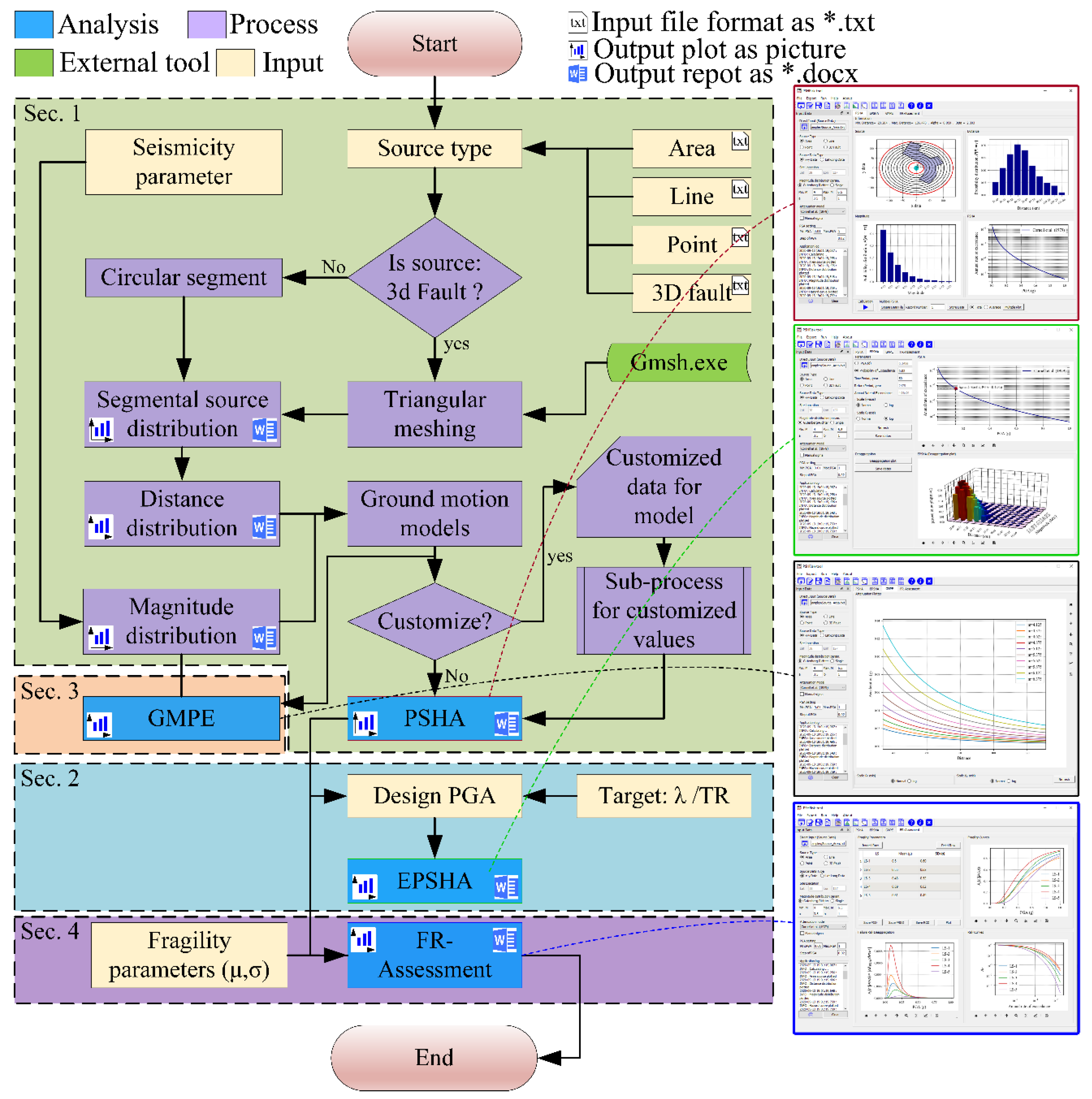
In the PSHRisk-tool, the Python language has been used to implement the above described theories and algorithms to fulfill the main purpose. The operation process, the features and system architecture are explained here by the flowchart as shown in Figure 4 along with the necessary explanation. The main GUI is divided into the following main sections:
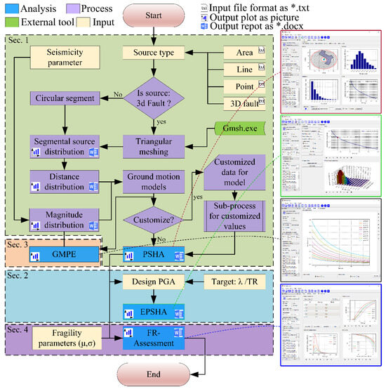
Figure 4.
PSHRisk-tool flowchart showing the whole process along with output GUI.
- Section 1: Probabilistic Seismic Hazard Analysis (PSHA)
- Section 2: Extended Probabilistic Seismic Hazard Analysis (EPSHA)
- Section 3: Ground Motion Prediction Equation (GMPE)
- Section 4: Failure Risk Assessment (FR-Assessment)
The GUI has a main input panel, by which it will give the user access to input the source data in “*.txt” format. This tool can model four types of sources such as point, line, area and 3D fault by containing the source information either by Cartesian coordinates or by geographic coordinates (latitude and longitude). A button on the main panel will allow inputting the “txt” file for the source data. Except for the 3D source, the source distance from the site is automatically divided into ten parts. 3D fault source “txt” file consists of the three-dimensional ordinates of a given fault plane from the site by providing the mesh sizes and strikes angle. After selecting the source type, the following sequence will introduce the systematic PSHRisk tool features:
3.1. Section 1: Probabilistic Seismic Hazard Analysis (PSHA)
As explained in the methodologies in previous sections, the PSHA curve for a definite GMPE (attenuation) model depends on a definite seismic parameter. The user needs to input the seismicity constants like a, b and slip rates and as well as the magnitude of interest range. For each attenuation, the model has an individual popup interface to input the required soil condition of the site such as soil type, share wave velocity of the top of subsurface profile (), fault mechanisms, etc. This tool is dedicated to showing the single source PSHA as well as multiple source PSHA. By selecting a PGA range through the input panel and using the selected attenuation equation, this window will show the segmental view of the source, distance and magnitude distribution for the individual source (point, line, area, and 3D fault).
In the case of line and area source, the source-to-site distance is coded in such a way so that these can show fixed equal ten segments between the shortest circle and the longest circle from the site. As a result, the ten bars in the plot express the probability density function for distance and magnitude .
Then, the probability of exceedance is determined using strong GM models, where PSHRisk-tool accumulated 21 default attenuation models (GMPE). To allow the selection of GMPE to draw the hazard curve, the PSHRisk-tool will show the sub-popup-interface for each attenuation model. The single source PSHA as well as multiple sources PSHA has been adopted here to show the mean annual rate of exceedance always in terms of PGA with any user-defined range and increment. In this part of the tool, the lambda (λ) calculated for a single source can be saved in an EXCEL spreadsheet and the multiple sources lambda (λ) (total or heavy average) can be calculated by recalling the EXCEL spreadsheet stored.
3.2. Section 2: Extended Probabilistic Seismic Hazard Analysis (EPSHA)
Another name of extended probabilistic hazard analysis (EPSHA) part is deaggregation, which is presented by the 2nd tab named “ESPHA” for plotting the hazard contribution with a pair of distance and magnitude. The hazard contribution can also be shown for magnitude and distance solely. Here except the main panel, another panel is customized to input the time period, the return period (TR) and so on. The different return periods will show different contributions to hazard by the 3D deaggregation plot because the hazard contribution is the ratio of an individual probability distribution function to the total probability distribution function for that specific return period.
3.3. Section 3: Ground Motion Prediction Equation (GMPE)
The graphical representation of this part is coded according to the existing attenuation model to examine the effect of various parameters. Alongside, it also shows the variation of acceleration in terms of distance and magnitude . The tool accounts for ground motion variability and allows the retrenchment of the ground motion distribution at a user-defined number of standard deviations.
3.4. Section 4: Failure Risk Assessment (FR-Assessment)
This tab named as “FR-Assessment” indicates the assessment of the mean annual frequency of exceedance for different structural damage. A customized panel has been created in this tab to input necessary data and it allows the fragility parameters from seismic failure probability of any infrastructure. To analysis the failure risk, this tool allows the user to input the fragility parameters (Mean and standard deviation). The previously calculated annual rate of exceedance for a given site is then combined with the fragility failure data as textualized by python language using the existing theory explained in Section 2.6. This FR-Assessment will help to identify the most vulnerable point in a massive structure like a dam, nuclear power plant containment, etc. By adopting an area source, the flowchart presented in Figure 4 shows the whole process and the illustrative output on the right side of the flowchart.
3.5. About System Architecture
PSHRisk-tool is developed as stand-alone exclusively for Microsoft Windows operating systems fully written in a python programming language. To make a tidy GUI and for numerous mathematical and logical evaluations, PyQt5 has been used, which is one of the most popular Python bindings for the Qt cross-platform C++ framework explained in Riverbank Computing Limited [47]. The following system architecture has been considered to make this tool:
3.5.1. GUI
It involves partial pre-processing, processing and post-processing. In the case of pre-processing only source coordinates, data need to import as a text file and other data can be assigned through GUI. The GUI is designed to provide an exchange relationship between the user and the analysis component. The GUI of PSHRisk-tool is very simple and students/researchers/engineers/ professionals can use without having deep computer skills. It is very handy and a user can export all analysis data and plot easily.
3.5.2. Python Module
Graphs are plotted using matplotlib [48] and can be exported at every step. The segmental distribution analysis of the area and line source is implemented by Shapely. Shapely is based on the widely deployed GEOS and JTS libraries [49]. In the case of 3D faults, a triangular meshing system has been applied. Because triangular meshes allow the application of more complicated geometry of the seismic source. To generate the mesh of faults pygmsh [50] module is exploited. Pygmsh performs the meshing process by calling Gmsh.exe [51]. For exporting the report in each step python-docx module is used, which is powerful for creating Microsoft Word documents. Openpyxl [52] is utilized to create an Excel file. This excel file perform to store data and plot for multiple hazard analysis.
3.5.3. Caching Scheme
Caches are that tool features which store data for use. This tool accumulates all input and analysis result data in a cache. Users can access or modify the caches data in any next steps.
3.5.4. Exporting Facility
An essential component that provides exporting the output data or graphs for further analysis, modification, or investigation as a researcher. Users can export the data in Microsoft Word and Excel format.
4. Verification of PSHRisk-Tool Results
4.1. Analytical Solution
PSHRisk-tool capable of solving general cases that involve source layouts, seismic ruptures and ground motion prediction equations. To define the fidelity and validity of the PSHRisk-tool, an example containing three different sources in a site has been adopted here from Kramer [37]. In this example assumed that the earthquakes of magnitude less than 4 do not contribute to the seismic hazard, where Table 2 and Figure 5 represent the detailing of the seismic parameters.

Table 2.
Source information of the example.
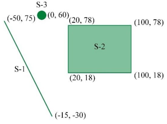
Figure 5.
A seismic site with three different sources.
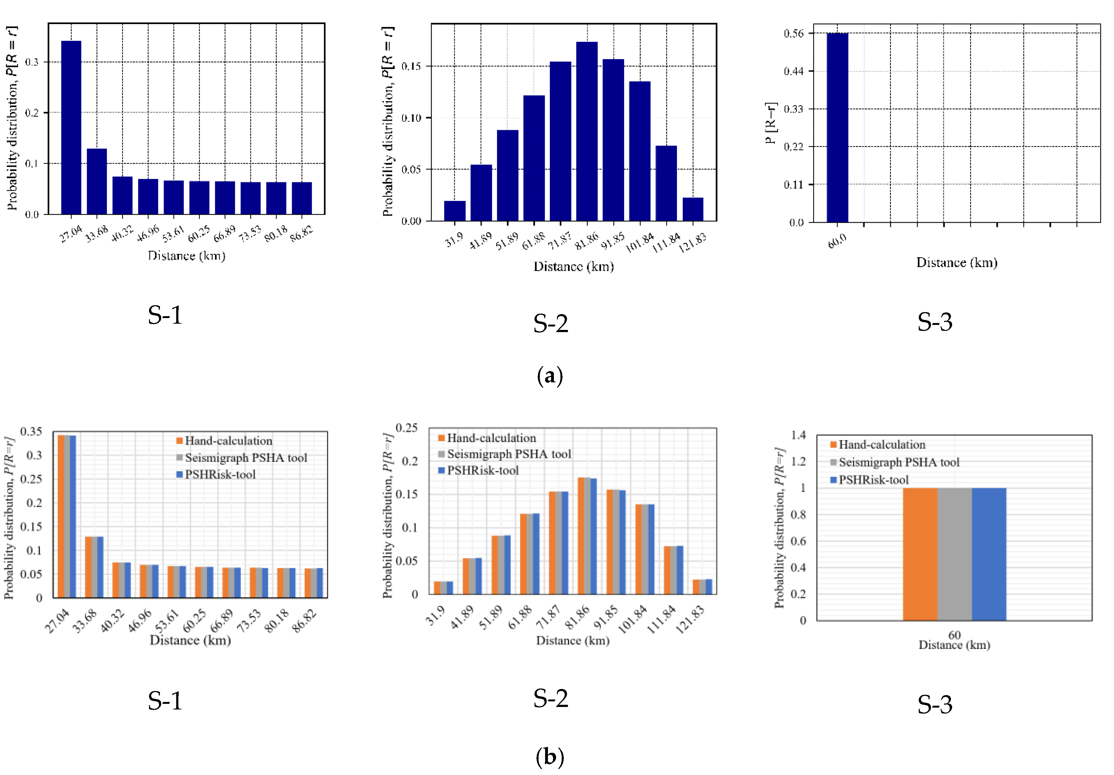
With the same example, verification has also been done by commercial software “Seismograph PSHA tool” [53] for accuracy, which is followed by the classical PSHA rules for seismic hazard analysis. The probability distribution for sources is coded here by using the equal circular grids as shown in Figure 2 division between the minimum and maximum fault distance from the site. The code adopted the 10 fixed segmental division and the portion of source fallen in that segment is counted for the probability distribution function.
As in PSHA, all sources of earthquakes are assumed to be capable of generating damaging situations at the site, so before getting the seismic hazard curve, the probability distribution for source-to-site distance is conducted. Alongside this, the magnitude distribution also has been adopted because of the different magnitude range for each source. Based on the theory explained in the above sections, the result from the PSHRisk-tool is compared with hand calculation and “Seismograph PSHA tool”.
The maximum error in the result of the probability distribution has been observed from Figure 6 is 0.96% (among all sources) considering three sources, which is very negligible and acceptable. Besides, in magnitude distribution, Figure 7 presents a zero-difference comparing with the references for each source.

Figure 6.
Verification for the probability distribution of distance, (a) PSHRisk-tool view, (b) Comparison.


Figure 7.
Verification for the probability distribution of magnitude with truncated Gutenberg-Richter relationship, (a) PSHRisk-tool view, (b) Comparison.
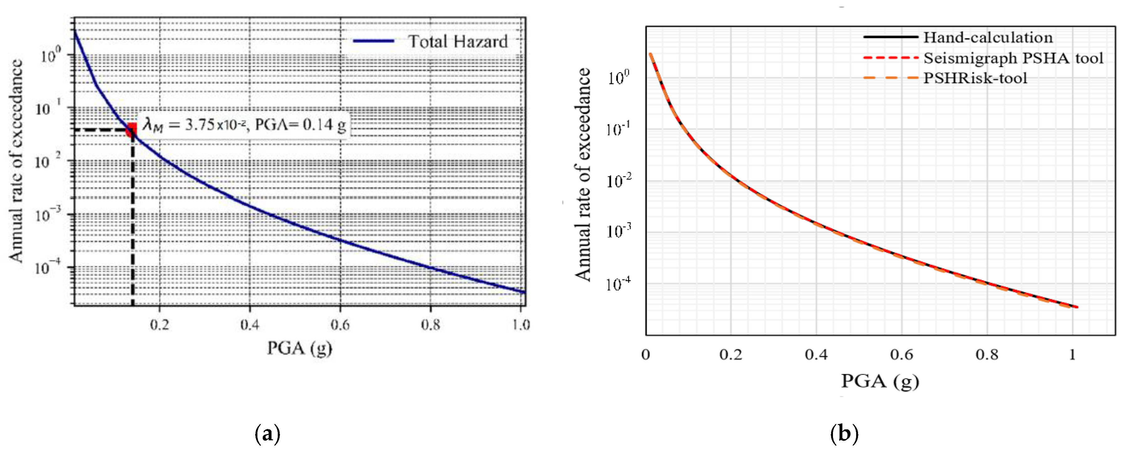
The predictive GMPE model for verification has been focused on Cornell et al. [22] as a GM model to calculate the PGA at the seismic site. The corresponding annual rate of exceedances will be integrated taking the probability distribution of source-to-site distances and magnitudes along with the earthquake rate using Equation (10). However, the result generated by this tool in Figure 8, shows approximately the same result as the hand-calculation from Kramer [37] and the commercial software “Seismograph PSHA tool” [53]. Up to the seismic hazard curve, PSHRisk-tool exposed a similar output with the hand-calculation. Now, for reducing the manuscript length the validation of EPSHA is carried out only for the area source. In the “Seismograph PSHA tool” as there is no deaggregation part, so in EPSHA verification is only compared with the hand calculation.

Figure 8.
Seismic hazard curve for verification, (a) PSHRisk-tool view, (b) Comparison.
Deaggregation is the contribution of the annual rate of exceedance for a given intensity measure . It can solely focus on the magnitude or source-to-site distance and this section shows the pair deaggregation of hazard contribution. In Figure 9a, the blue bars indicate the contribution of hazard for hand-calculation and the green bars indicate the hazard contributions for PSHRisk-tool. The PGA level, which will be exceeded by an earthquake with a given magnitude, can be visualized by this deaggregation curve, in which it is understandable that for a low magnitude the contribution may be high or vice versa.
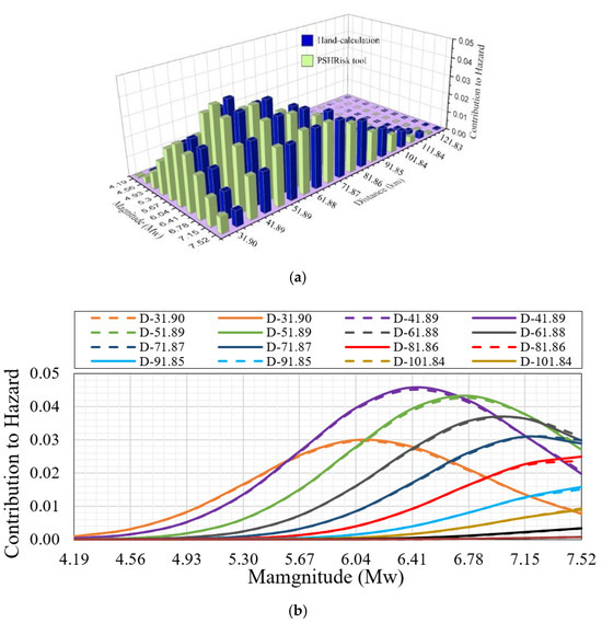
Figure 9.
Verification of hazard deaggregation for PGA > 0.16 g: (a) 3D plot, (b) Plot for focusing CoV; D = Distance (km).
As we observe in Figure 9a, the blue bars and green bars for a specific magnitude and distance expressed here almost the same result. Besides this, Figure 9b shows the clear visualization of the coefficient of variation (CoV) between the deaggregation results of the hand-calculation and the PSHRisk-tool. In Figure 9b, the dotted lines show the hand-calculation and solid lines focus on the proposed tool result. After analyzing the comparison, a small CoV has been detected, especially in the pick point of each deaggregation curve, which has a maximum value of 0.033.
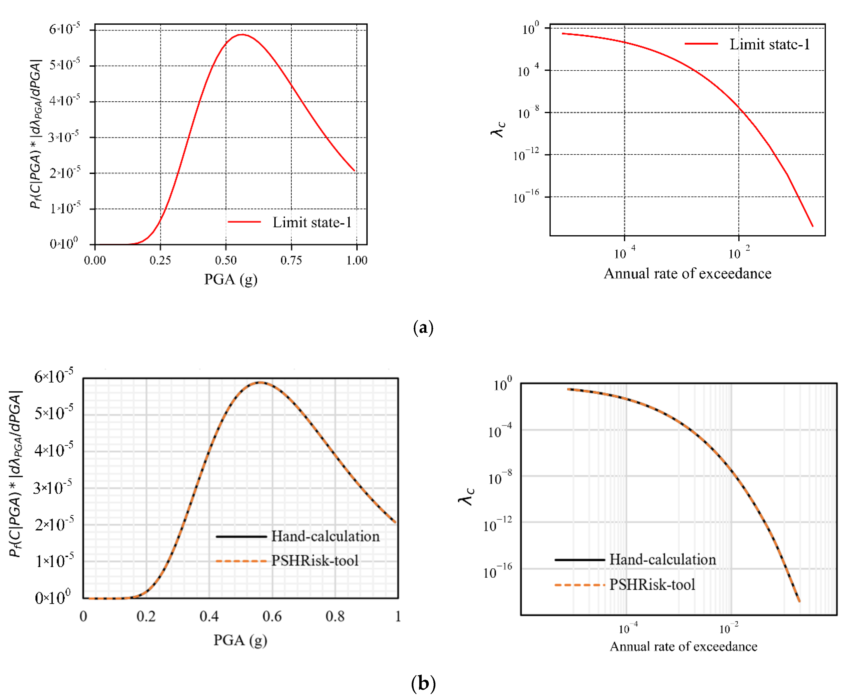
If the user has the structural seismic response like mean and standard deviation of the fragility parameter, this tool can assess the failure risk of that structure. To verify this part, the fragility parameter has been taken in this study for a building structure from Eads et al. [3] and these are 0.96 (median collapse intensity) and 0.39 (lognormal standard deviation). By using Equation (18), the failure risk assessment has been calculated here by combining with the lambda (λ) value for the area source (Figure 5). The result is shown in Figure 10 indicates the same result with hand calculation, which is acceptable for verification.
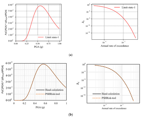
Figure 10.
Verification of failure risk assessment curve, (a) PSHRisk-tool view, (b) Comparison.
4.2. Existing Test Model
The verification of a PSHA tool is essential to assure that the analysis results are reliable. The analytical verification process of PSHRisk-tool has been carried out in Section 4.1 considering three types of sources i.e., area, line and points. An additional test case from Danciu et al. [54] is also considered for validation.
PSHRisk-tool performs well under the framework of the selected case and is suitable for the development of probabilistic seismic hazard analyses as well as for further EPSHA and seismic risk assessment.
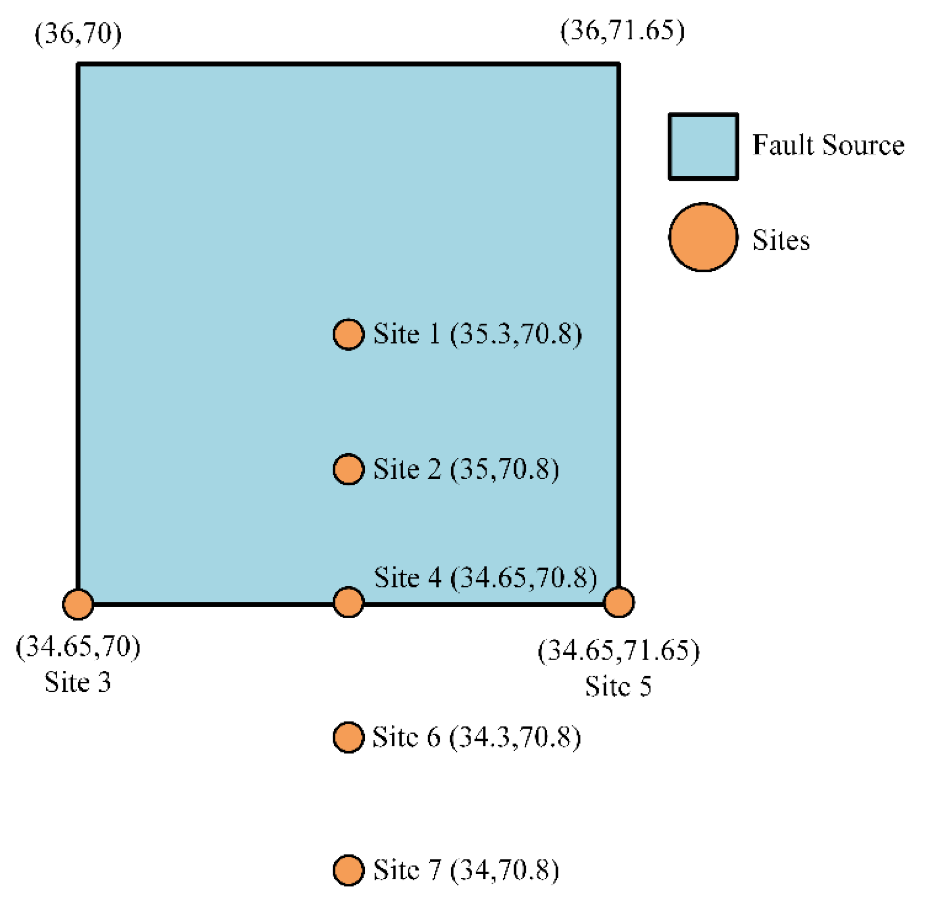
The basic information for this case is shown in Figure 11 and Table 3. More detailed information related to this tested case can be found in the GEM technical report “GEM1 Hazard: Overview of PSHA Software” [54].
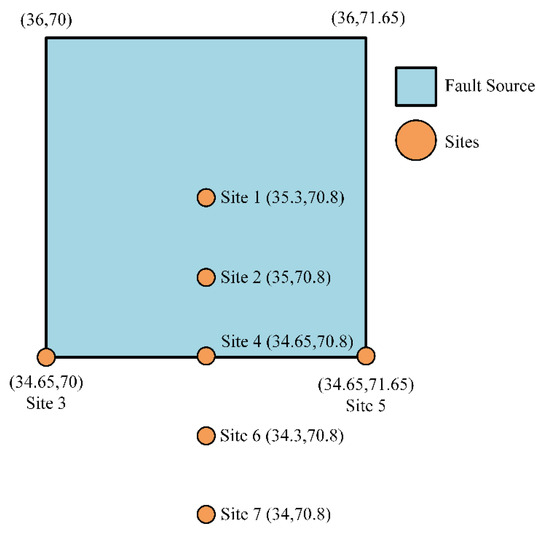
Figure 11.
Area source-based test geometry and sites.

Table 3.
Area source-based test case details.
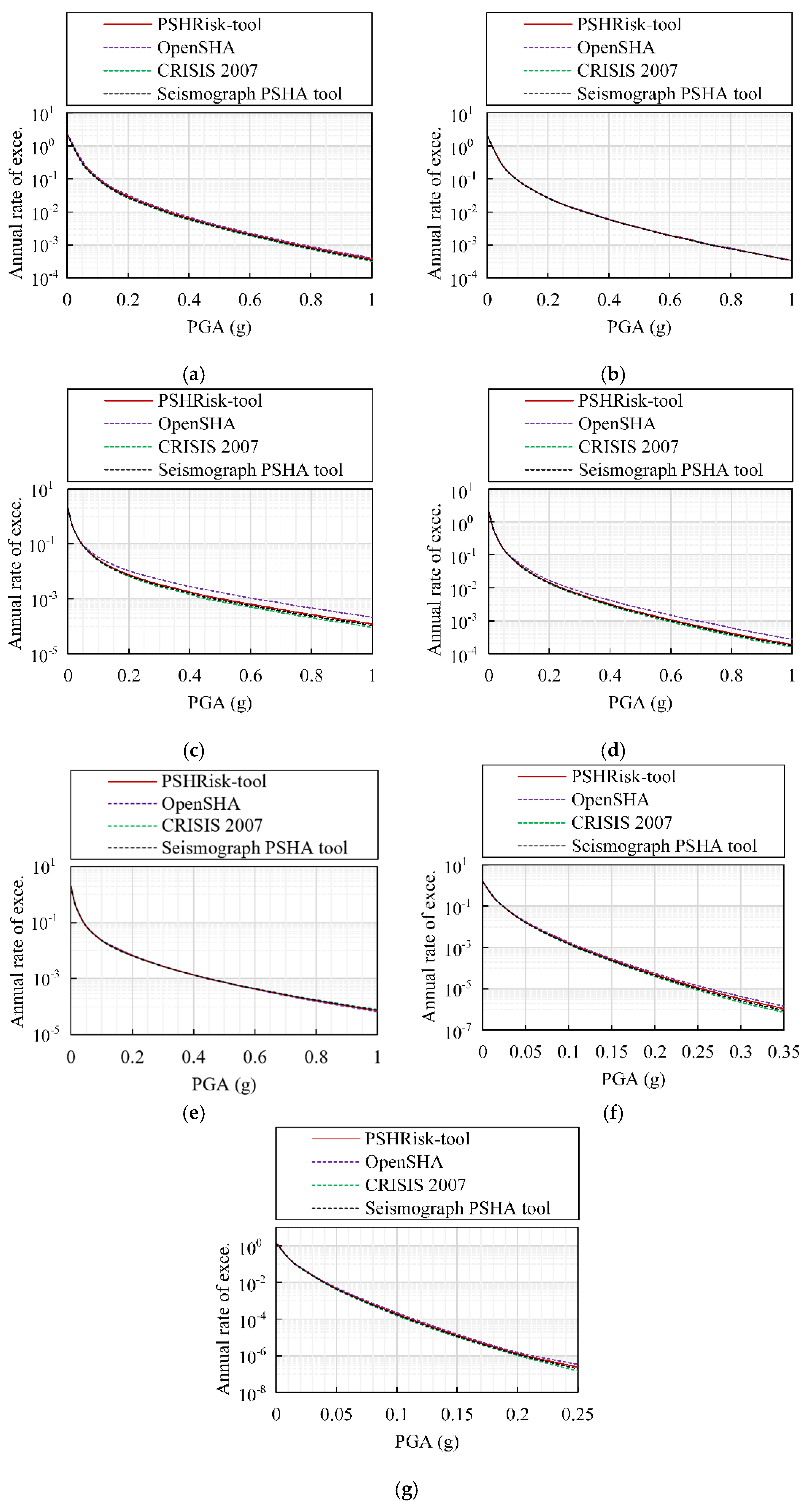
For the single site of this test case, the magnitude distribution plot will same for all sites, but site-to-source distance distribution will change. Therefore, for site 1 up to the seismic hazard analysis, all steps have been shown in Figure 12. For the rest of the sites, Figure 13 and Figure 14 show segmental views and probability density function of distance, respectively. To reduce the paper length the result has been shown up to the hazard curve for all sites and for comparing the seismic hazard curve between PSHRisk-tool and other reference software, the same graph has been used as shown in Figure 15.
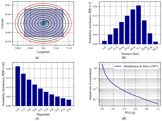
Figure 12.
(a) Segmental view of area source, (b) Probability density function of distance, (c) Illustration of probability density function for magnitude for a source with a truncated Gutenberg–Richter distribution, (d) Probabilistic seismic hazard curve, respectively for Site 1 by PSHRisk-tool.


Figure 13.
Segmental view of area source by PSHRisk-tool for, (a) Site 2, (b) Site 3, (c) Site 4, (d) Site 5, (e) Site 6, (f) Site 7
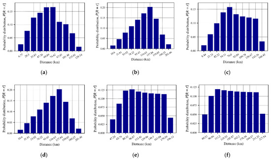
Figure 14.
Probability density function of distance PSHRisk-tool for, (a) Site 2, (b) Site 3, (c) Site 4, (d) Site 5, (e) Site 6, (f) Site 7.
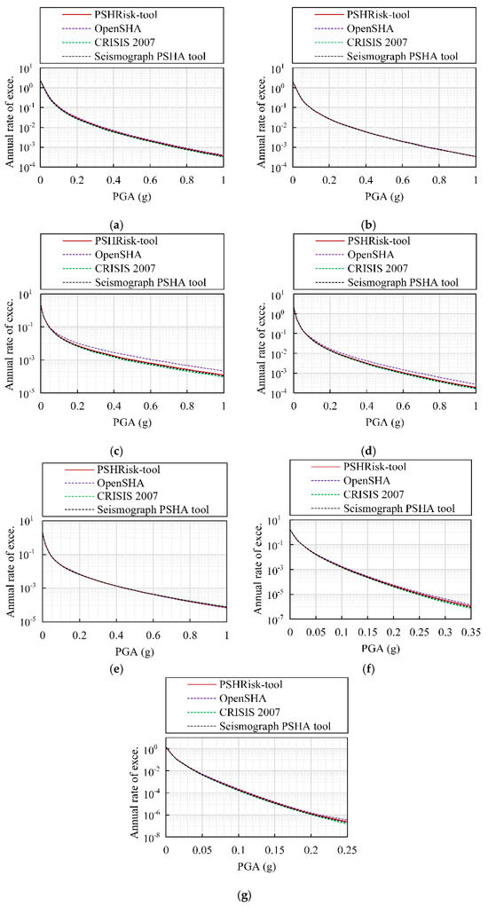
Figure 15.
Hazard curves for area source-based test case, (a) Site 1, (b) Site 2, (c) Site 3, (d) Site 4, (e) Site 5, (f) Site 6, (g) Site 7.
The selected test case is conducted considering the following software: OpenSHA, CRISIS 2007 and seismograph PSHA tool for the validation of the developed PSHRisk tool. The hazard curves obtained from different PSHA software for each site are shown in Figure 15, which shows that the analysis results are very similar to those of the CRISIS 2017 and Seismograph PSHA tool. Only for two sites (3 and 4), the result obtained from OpenSHA gives slightly higher values which show a similar statement as explained in Danciu et al. [54].
From the above analysis of the PSHRisk-tool results with the analytical example and other software, it is optimized that the tool is suitable for the determination of PSHA and FR-Assessment.
5. Case Study and Discussion
In addition to introducing the application and proper verification, the efficient and full performance of this tool is explained briefly through a case study. The main objective of this section is to discuss the results of the case study. To achieve the objective, an investigation is conducted on models of seismic sources in South Korea and it is made from a historical and instrumental earthquake catalog from Choi et al. [55]. The Gunnam concrete gravity dam in South Korea is selected as the site by taking the latitude and longitude value (38.104° N and 127.021° E).
The site-specific magnitude is appropriate for use in seismic risk assessment because there are only a few strong GM data and seismological information for the dam sites in South Korea. Table 4 displays the range of magnitude as well as the seismicity parameters corresponding to “Source ID” of the seismic source models. For the magnitude–frequency relationship, Gutenberg–Richter relation [38] is considered for each area source. Table 5 presents the value of latitude and longitude for each seismic source of the corresponding selected source model (here taken M-B seismic model in South Korea) [56].

Table 4.
Seismicity parameters.

Table 5.
Seismic source coordinate for model M-B
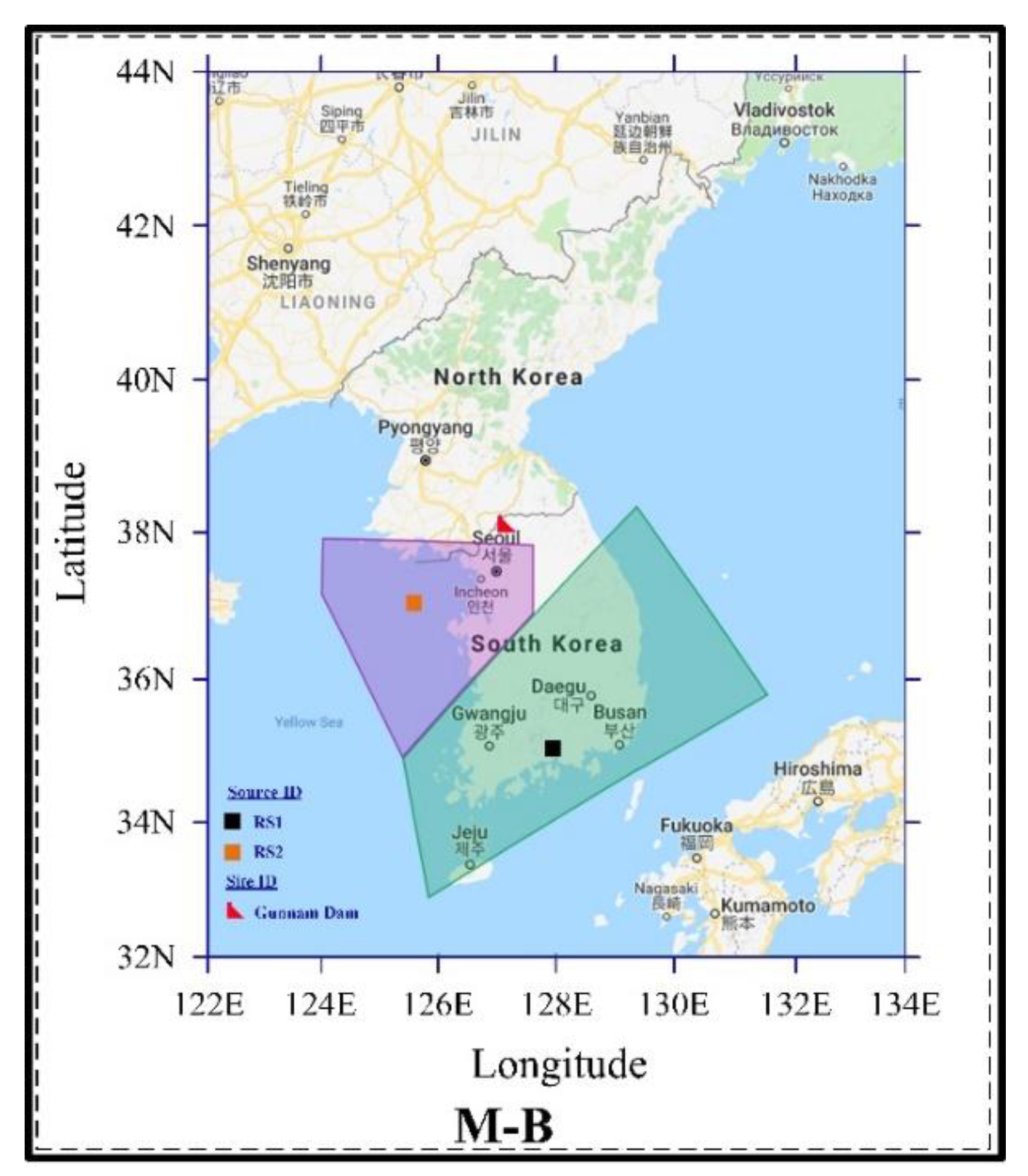
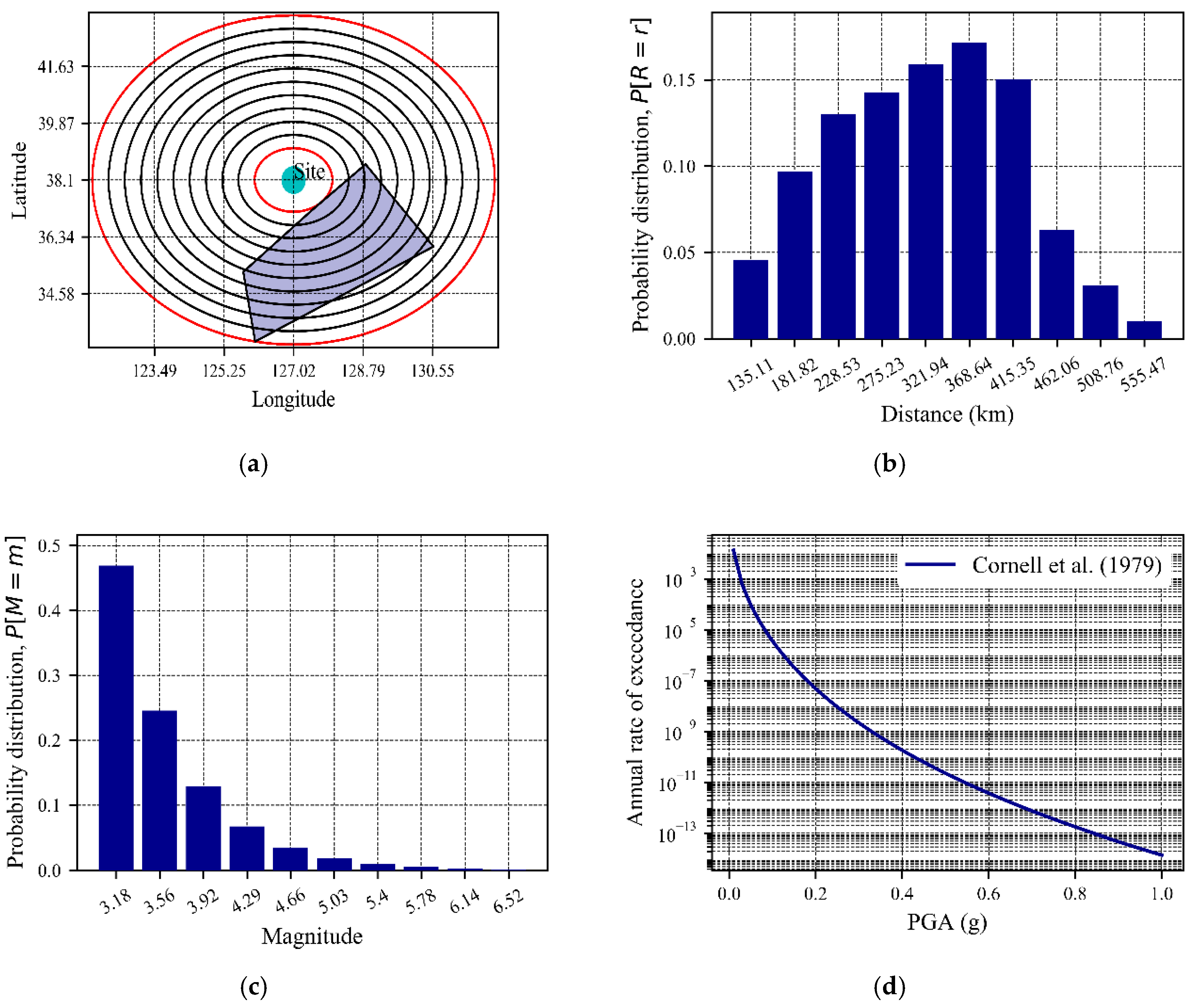
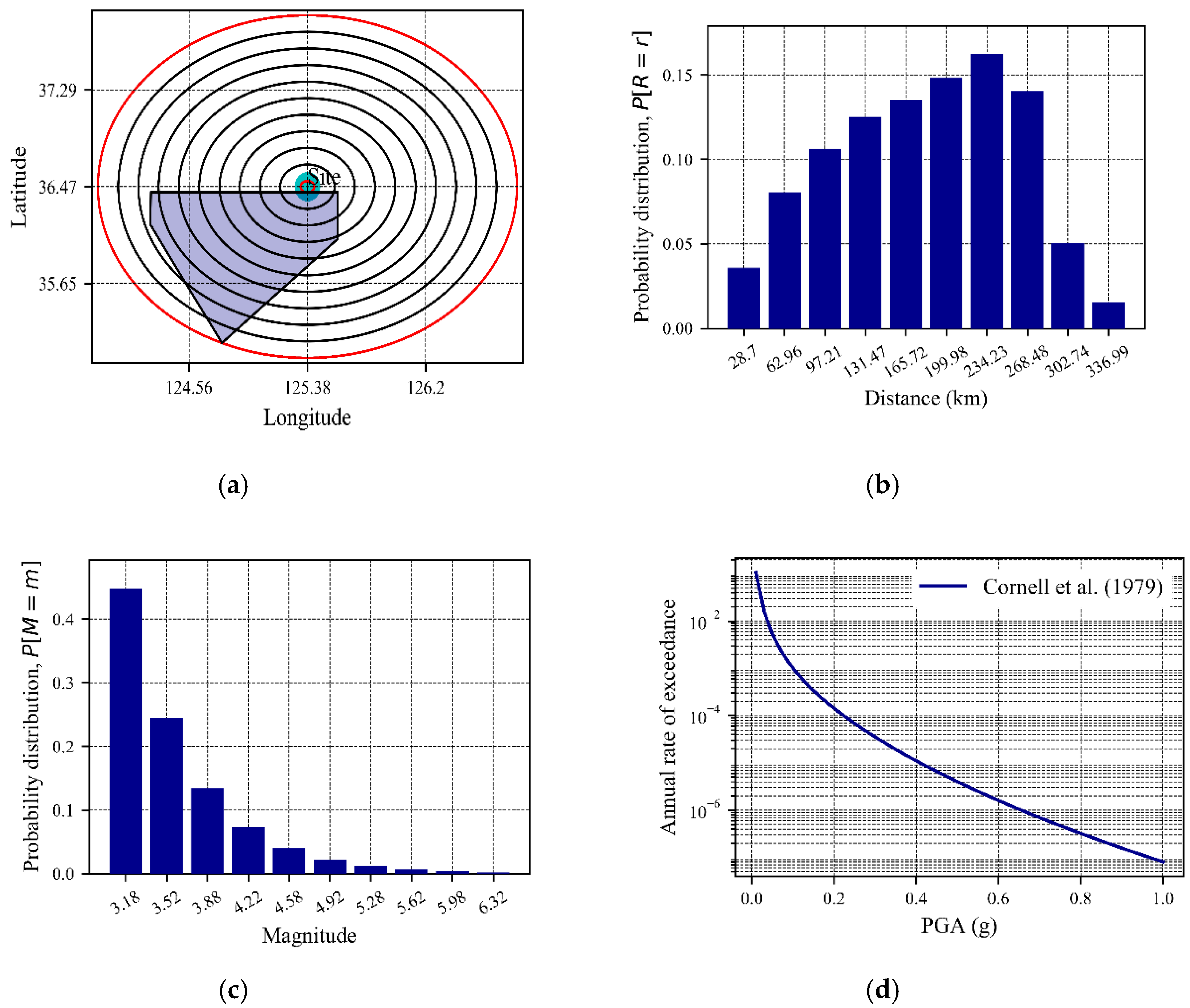
Among several earthquake records, this seismic source model (M-B) recorded two major sources, which are identified here as RS1 and RS2 in Figure 16 [57]. After operating with the input data as the maximum and minimum values of magnitude from Table 4, Figure 17 explains the 10 segmental views of area source, distribution of source-to-site distance and magnitude and single-source hazard curve for RS1. Similarly, Figure 18 shows the illustration for RS2.
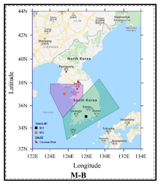
Figure 16.
Seismic source model for probabilistic seismic hazard analysis of South Korea showing the affected area of earthquakes produced by accounting more than 1800 historical earthquakes records. The boxes indicate the source identification; the transparent portions show the boundary of the affected area and the dam icon focuses on the site location on the map.

Figure 17.
(a) Segmental view of area source, (b) Probability density function of distance, (c) Illustration of probability density function for magnitude for a source with a truncated Gutenberg–Richter distribution, (d) Probabilistic seismic hazard curve, respectively for RS1.
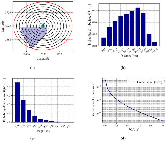
Figure 18.
(a) Segmental view of area source, (b) Probability density function of distance, (c) Illustration of probability density function for magnitude for a source with a truncated Gutenberg–Richter distribution, (d) Probabilistic seismic hazard curve, respectively for RS2.
Figure 17b and Figure 18b show the characterization of source-to-site distance from the RS1 and RS2 to the Gunnam dam. The site was near about the source RS2 and far from the RS1, as a result, the average 283 km showing a 0.80 for the probability of occurrence. Except for this, the probability distributions for the distance between 28.7 and 555.47 km varies approximately from 0.024 to 0.160 (Figure 17b and Figure 18b). Analyzing Figure 17c, the increasing pattern has been shown in the exponential of the probability distribution, which is found 0.01 at the magnitude of 6.38 to 0.38 at a magnitude of 4.12 for RS1.
Similarly from Figure 18c, the increased value is found from 0.02 at the magnitude of 6.38 to 0.35 at a magnitude of 4.12. Consequently, the plots in Figure 17d and Figure 18d combine the probabilities of possible magnitude and distance distribution with suitable attenuation equation (here we used the Cornell, Banon and Shakal [22] as GMPE model) and with activity rate of the earthquake which followed here truncated Gutenberg–Richter relationship by hazard curves for RS1 and RS2, respectively.
Notably, the source-to-site distance is affecting the exceedance rate, in which RS2 shows the maximum annual rate of exceedance is almost with a minimum value of and RS1 delivered approximately with a minimum value of . These results present that the received seismic region is mostly affected by RS2.
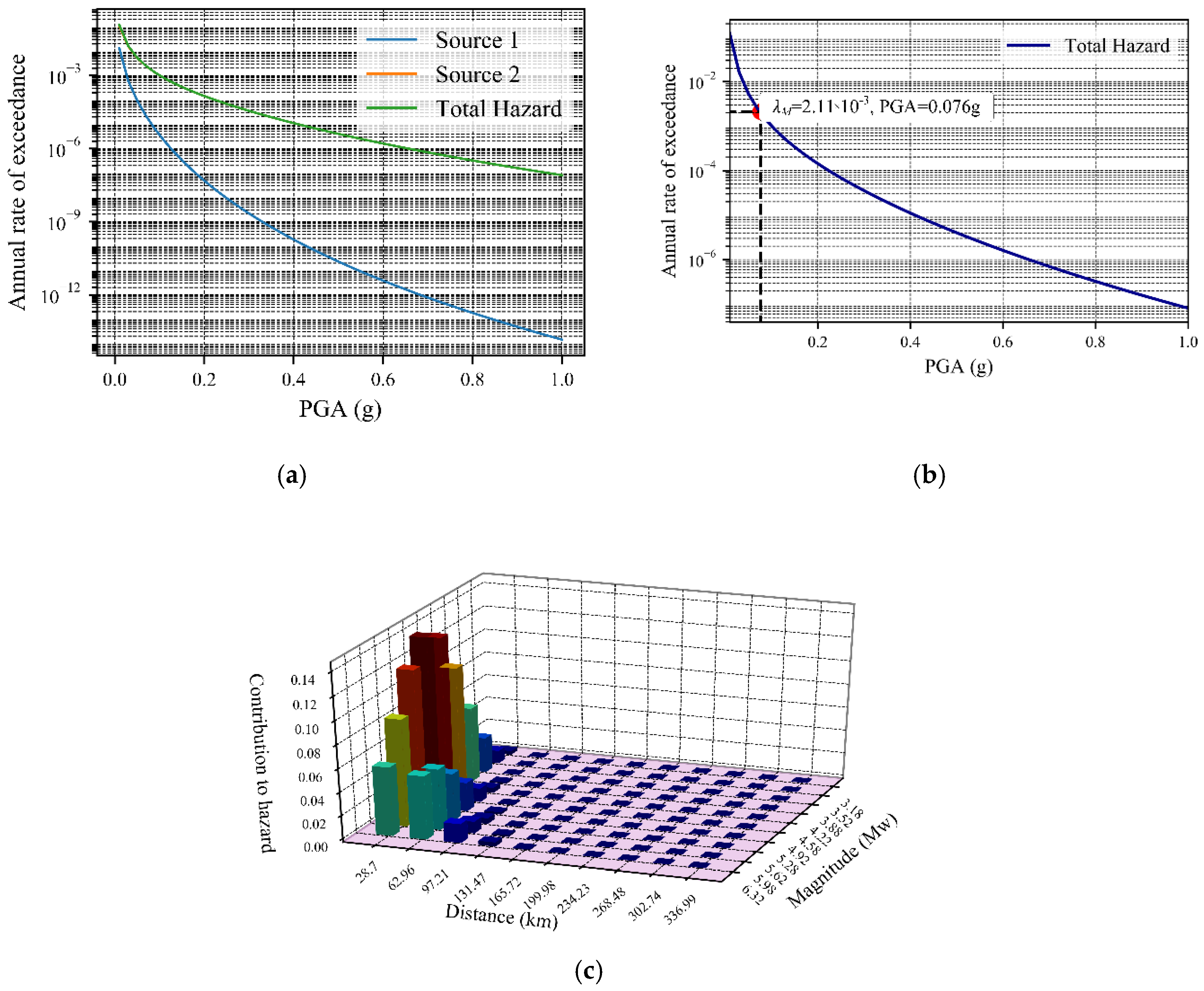
This tool calculates the hazard curve for a single source as well as the total hazard curve of all sources. However, as the source type was an area; therefore, Figure 19a reports the total hazard curves along with the single source hazard curve. As previously discussed, that the seismically most affected source is RS2, therefore in Figure 19a, the total hazard curve overlapped on the hazard curve of RS2 (calculated total hazard curve is almost equal to the RS2). Consequently, the deaggregation plot is emphasized here for source RS2 in Figure 19c. The horizontal dotted line in the annual rate of exceedance equal to 0.00211 for 475 return period (TR) shows the peak ground acceleration (PGA) of 0.076g as shown in Figure 19b.
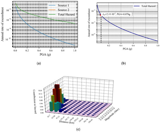
Figure 19.
(a) Seismic hazard curve for all sources along with total hazard curve, (b) Total hazard curve showing the annual rate of exceedance to the corresponding 475 returned period (TR), (c) Deaggregation of PGA with 475 years TR for RS2.
From the deaggregation plot of the seismic site, it can be found that the nearer source-to-site of an earthquake zone will contribute more to the hazard than the remote source, but the magnitude affects the contribution in a different manner as the magnitude distribution follows recurrence law. As a result, Figure 19c shows here approximately the range of magnitude is 4 to 5 for contributing to hazard. Even though the case study has been carried out for the Cornell, Banon and Shakal [22] attenuation equation in hazard distribution, the other specific choices of GMPE models are available in PSHRisk-tool.
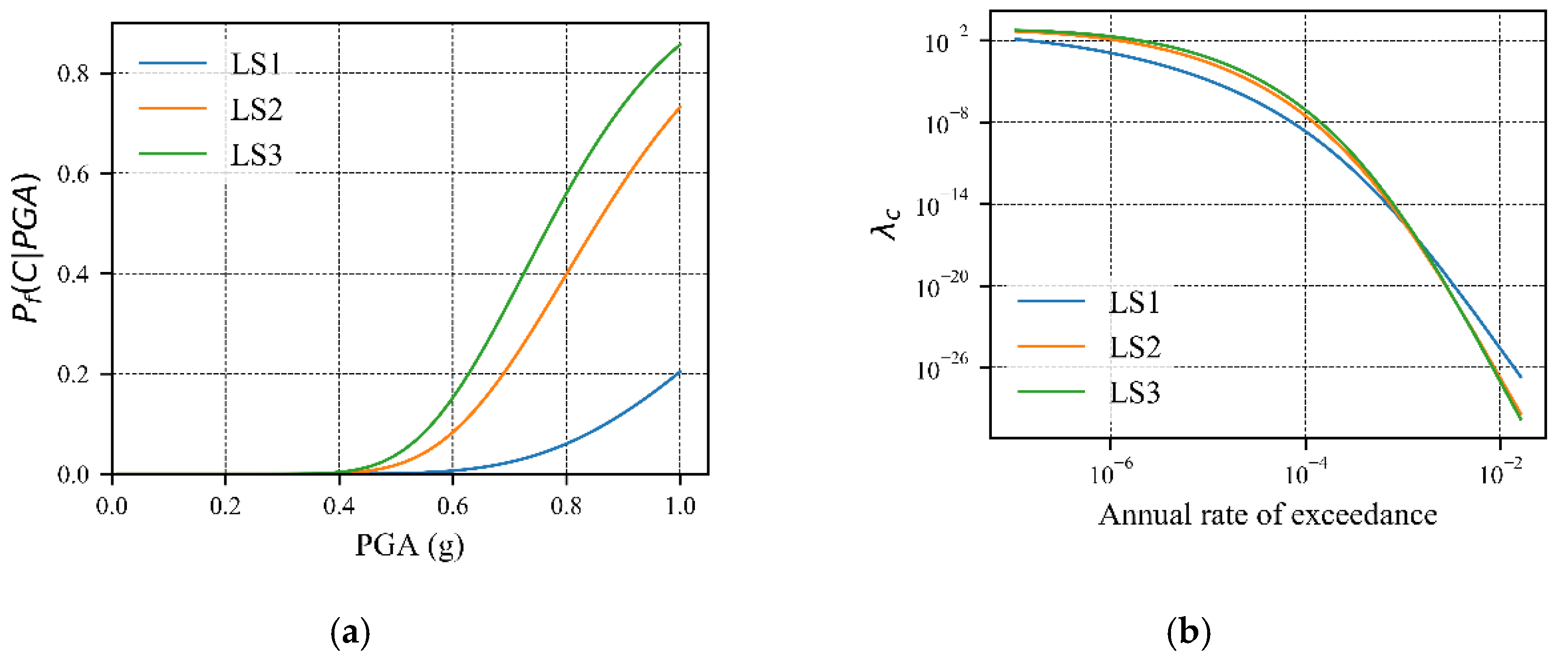
For discussing the result of the FR-Assessment of the required case study, the fragility parameters are determined (for the considered Gunnam concrete gravity dam in South Korea) at first from the existing software ABAQUS. The fragility parameters for different damage stages such as tensile crack at the neck (LS1), relative displacement at the top of the dam (LS2) and tensile crack at the base (LS3) are 1.29, 0.854 and 0.771 for a mean (μ) value and 0.308, 0.255 and 0.244 for a standard deviation (σ), respectively. These values are observed and taken as the input value for FR-Assessment. As shown in Figure 19b, the total hazard curve is then combined with the failure probability expressed in Figure 20a for different damage stages.
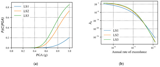
Figure 20.
(a) Fragility analysis of structure in the site for different damage stages; (b) Failure risk curve.
The largest risk contributions in each limit state happen in 0.80 g, 0.70 g and 0.62 g for LS1, LS2, and LS3, respectively. If it is figured out in the fragility curve for corresponding peak value in the failure risk assessment, it will focus on the probability of failure around 7.5%, 23% and 22% for LS1, LS2, and LS3, respectively. For LS1 the area under the FR-assessment curve between 0 and 0.90 g is 70%, which is dominated by the lower portion of the fragility curve for the corresponding higher-intensity. Similarly, the covered area for LS2 and LS3 can be determined and these are 80% and 80%, respectively. This percentage will vary from structure to structure, because of the steep slope in the hazard contribution at the same intensities of ground motion of the corresponding small probabilities of failure.
Finally, from Figure 20b, it is depicted that the probability that a structure will be destroyed when any level of earthquake occurs in a particular area, which can be solved by the failure risk assessment.
6. Conclusions and Future Work
This study introduces students/researchers/engineers/professionals to a new software named PSHarsk-Tool, which can calculate PSHA and FR-assessments by a user-friendly and flexible GUI. This is the original v1.0 version fully scripted in Python code as stand-alone exclusively for the Microsoft Windows operating system.
In this paper, sequentially at first, the previous PSHA software has been discussed, then the necessary theories and algorithms to build the PSHRisk-tool have been explained. By implementing these algorithms in Python-language, the result from this tool is verified through analytical and existing test models. Accounting for almost all the attenuation models for considering different fault mechanisms in the seismic zone, it can handle whole features related to PSHA. After inserting the coordinates or latitude and longitude at any seismic zone, it can characterize the source-to-site distance as well as the probability distribution. The frequency-magnitude for the different source magnitude of the probability distribution shows an exactly correct distribution with the existing algorithm.
In the case of hazard analysis, the operator can get the hazard curve for a single source or multiple sources. The seismic hazard curve shown by this tool is synchronized with the GM as PGA even the attenuation model would be calculated in spectral acceleration. For calculating the contribution of hazard in the site, a specific GM for a specific return period can be done by the classical extended PSHA or hazard deaggregation plot. Except for the conditional hazard curve, this will show the deaggregation of any return period along with the threshold IM value. In the GMPE portion of this tool, the parametric effects for a seismic site can be analyzed with the pair of distance and magnitude variations. It can determine the hazard curve for any GMPE model, which made it vaster overall.
The addition of estimating the structural failure risk can handle and illustrate the risk contribution for a vulnerable IM of any infrastructure along with site-specific hazard analysis. If the fragility analysis for different damage levels can be included as an input value, it can calculate the failure risk combining the fragility curve with the single hazard or total hazard distribution. To demonstrate this combined package of the tool is the challenging issue of this manuscript. To find the software details user can go to the link mentioned in the “Supplementary Materials” section of this manuscript.
With due limitations, the authors tried to introduce the initiation of the present work. In the future version of this tool will include the conditional hazard distribution, different IMs, other characterized fault types, the logic tree as well as will improve the visibility of the tool. Up to now, this version allows access only for Microsoft Windows operating systems, but in the future, the authors will make it accessible for Linux or Mac OS users.
Supplementary Materials
For the test of the user, the setup file, user manual and excel file for verification of the example presented in this manuscript, etc. can be found online at http://www.kim2kie.com/3_ach/PSHRisk-tool/PSHRisk_tool.php.
Author Contributions
Conceptualization, T.T.N. and M.M.R.; Formal analysis, T.T.N. and M.M.R.; Funding acquisition, D.K.; Methodology, T.T.N.; Project administration, D.K.; Software, T.T.N. and M.M.R.; Supervision, D.K.; Validation, T.T.N., M.M.R. and D.K.; Writing—original draft, T.T.N.; Writing—review & editing, T.T.N., M.M.R. and D.K. All authors have read and agreed to the published version of the manuscript.
Funding
This research was funded by the Korea Institute of Energy Technology Evaluation and Planning (KETEP) and the Ministry of Trade, Industry & Energy (MOTIE) of the Republic of Korea grant number no 20171510101960.
Acknowledgments
This work was supported by the Korea Institute of Energy Technology Evaluation and Planning (KETEP) and the Ministry of Trade, Industry & Energy (MOTIE) of the Republic of Korea (No. 20171510101960).
Conflicts of Interest
The authors declare no conflict of interest.
References
- Baker, J.W. An introduction to probabilistic seismic hazard analysis (PSHA). White Pap. Version 2008, 1, 72. [Google Scholar]
- Cornell, C.A. Engineering seismic risk analysis. Bull. Seismol. Soc. Am. 1968, 58, 1583–1606. [Google Scholar]
- Eads, L.; Miranda, E.; Krawinkler, H.; Lignos, D. Improved estimation of collapse risk for structures in seismic regions. In Proceedings of the 15th World Conference on Earthquake Engineering, Lisbon, Portugal, 24–28 September 2012. [Google Scholar]
- Eads, L.; Miranda, E.; Lignos, D.G. Average spectral acceleration as an intensity measure for collapse risk assessment. Earthq. Eng. Struct. Dyn. 2015, 44, 2057–2073. [Google Scholar] [CrossRef]
- Ibarra, L.F.; Krawinkler, H. Global Collapse of Frame Structures under Seismic Excitations; PEER Report 2005/06; The John A. Blume Earthquake Engineering Center: Stanford, CA, USA, 2005. [Google Scholar]
- McGuire, R. FRISK88M: User’s Manual; Risk Engineering Inc.: Louisville, CO, USA, 1996; p. 4155. [Google Scholar]
- Field, E.H.; Jordan, T.H.; Cornell, C.A. OpenSHA: A developing community-modeling environment for seismic hazard analysis. Seismol. Res. Lett. 2003, 74, 406–419. [Google Scholar] [CrossRef]
- Field, E.H.; Gupta, N.; Gupta, V.; Blanpied, M.; Maechling, P.; Jordan, T.H. Hazard calculations for the WGCEP-2002 earthquake forecast using OpenSHA and distributed object technologies. Seismol. Res. Lett. 2005, 76, 161–167. [Google Scholar] [CrossRef]
- Robinson, D.; Dhu, T.; Row, P. EQRM: An open-source event-based earthquake risk modeling program. In Proceedings of the AGU Fall Meeting, San Francisco, CA, USA, 10–14 December 2007. [Google Scholar]
- Youngs, R.R.; Coppersmith, K.J. Implications of fault slip rates and earthquake recurrence models to probabilistic seismic hazard estimates. Bull. Seismol. Soc. Am. 1985, 75, 939–964. [Google Scholar] [CrossRef]
- Pailoplee, S.; Palasri, C. CU-PSHA: A Matlab software for probabilistic seismic hazard analysis. J. Earthq. Tsunami 2014, 8, 1450008. [Google Scholar] [CrossRef]
- Abrahamson, N.A.; Silva, W.J. Attenuation of long period strong ground motions. In Proceedings of the Conference of American Society of Mechanical Engineers, Lakeland, FL, USA, 25 March 1993; p. 187. [Google Scholar]
- Abrahamson, N.; Silva, W.J. Empirical response spectral attenuation relations for shallow crustal earthquakes. Seismol. Res. Lett. 1997, 68, 94–127. [Google Scholar] [CrossRef]
- Ambraseys, N. Trends in engineering seismology in Europe. In Proceedings of the fifth European conference on earthquake engineering, Istanbul, Turkey, 22–25 September 1975; pp. 39–52. [Google Scholar]
- Ambraseys, N. Uniform magnitude re-evaluation of European earthquakes associated with strong-motion records. Earthq. Eng. Struct. Dyn. 1990, 19, 1–20. [Google Scholar] [CrossRef]
- Boore, D.M.; Joyner, W.B.; Fumal, T.E. Equations for estimating horizontal response spectra and peak acceleration from western North American earthquakes: A summary of recent work. Seismol. Res. Lett. 1997, 68, 128–153. [Google Scholar] [CrossRef]
- Campbell, K.W. Near-source attenuation of peak horizontal acceleration. Bull. Seismol. Soc. Am. 1981, 71, 2039–2070. [Google Scholar]
- Campbell, K.W. The dependence of peak horizontal acceleration on magnitude, distance, and site effects for small-magnitude earthquakes in California and eastern North America. Bull. Seismol. Soc. Am. 1989, 79, 1311–1346. [Google Scholar]
- Campbell, K.W. Empirical near-source attenuation relationships for horizontal and vertical components of peak ground acceleration, peak ground velocity, and pseudo-absolute acceleration response spectra. Seismol. Res. Lett. 1997, 68, 154–179. [Google Scholar] [CrossRef]
- Campbell, K.W.; Bozorgnia, Y. Updated near-source ground-motion (attenuation) relations for the horizontal and vertical components of peak ground acceleration and acceleration response spectra. Bull. Seismol. Soc. Am. 2003, 93, 314–331. [Google Scholar] [CrossRef]
- Campbell, K.; Bozorgnia, Y. Empirical ground motion model for shallow crustal earthquakes in active tectonic environments developed for the NGA project. In Proceedings of the 14th World Conference on Earthquake Engineering, Beijing, China, 12–17 October 2008; p. 4. [Google Scholar]
- Cornell, C.A.; Banon, H.; Shakal, A.F. Seismic motion and response prediction alternatives. Earthq. Eng. Struct. Dyn. 1979, 7, 295–315. [Google Scholar] [CrossRef]
- Donovan, N.C. A Statistical Evaluation of Strong Motion Data: Including the February 9, 1971 San Fernando Earthquake; Dames & Moore: San Francisco, CA, USA, 1973. [Google Scholar]
- Faccioli, E. Response spectra for soft soil sites. In Proceedings of the ASCE Geotechnical Engineering Division Specialty Conference, Pasadena, CA, USA, 19–21 June 1978. [Google Scholar]
- Faccioli, E. Engineering seismic risk analysis of the Friuli region. Boll. Geofis. Teor. Appl. 1979, XXI, 173–190. [Google Scholar]
- Joyner, W.B.; Boore, D.M. Peak horizontal acceleration and velocity from strong-motion records including records from the 1979 Imperial Valley, California, earthquake. Bull. Seismol. Soc. Am. 1981, 71, 2011–2038. [Google Scholar]
- Joyner, W.B.; Boore, D.M. Measurement, characterization, and prediction of strong ground motion. In Earthquake Engineering and Soil Dynamics II, Proceedings of the American Society of Civil Engineers Geotechnical Engineering Division Specialty Conference, Park City, UT, USA, 15–18 August 1988; American Society of Civil Engineers: Reston, VA, USA, 1988; pp. 43–102. [Google Scholar]
- McGuire, R.K. Seismic ground motion parameter relations. J. Geotech. Eng. Div. 1978, 104, 481–490. [Google Scholar] [CrossRef]
- Orphal, D.; Lahoud, J. Prediction of peak ground motion from earthquakes. Bull. Seismol. Soc. Am. 1974, 64, 1563–1574. [Google Scholar] [CrossRef]
- Sadigh, K.; Chang, C.-Y.; Egan, J.; Makdisi, F.; Youngs, R. Attenuation relationships for shallow crustal earthquakes based on California strong motion data. Seismol. Res. Lett. 1997, 68, 180–189. [Google Scholar] [CrossRef]
- Zare, M.; Sabzali, S. Spectral attenuation of strong motions in Iran. In Proceedings of the Third International Symposium on the Efects of Surface Geology on Seismic Motionn, Grenoble, France, 30 August–1 September 2006. [Google Scholar]
- Laouami, N. Vertical ground motion prediction equations and vertical-to-horizontal (V/H) ratios of PGA and PSA for Algeria and surrounding region. Bull. Earthq. Eng. 2019, 17, 3637–3660. [Google Scholar] [CrossRef]
- Podili, B.; Raghukanth, S. Ground motion parameters for the 2011 Great Japan Tohoku earthquake. J. Earthq. Eng. 2019, 23, 688–723. [Google Scholar] [CrossRef]
- Bajaj, K.; Anbazhagan, P. Determination of GMPE functional form for an active region with limited strong motion data: Application to the Himalayan region. J. Seismol. 2018, 22, 161–185. [Google Scholar] [CrossRef]
- Douglas, J. Ground Motion Prediction Equations 1964–2014; PEER Report 2011; University of Strathclyde: Glasgow, UK, 2014; p. 102. [Google Scholar]
- Medina, R.A.; Krawinkler, H. Seismic Demands for Nondeteriorating Frame Structures and Their Dependence on Ground Motions; PEER 2003/15; Pacific Earthquake Engineering Research Center: Berkeley, CA, USA, 2004. [Google Scholar]
- Kramer, S.L. Geotechnical Earthquake Engineering; Pearson Education: Chennai, India, 1996. [Google Scholar]
- Gutenberg, B.; Richter, C.F. Frequency of earthquakes in California. Bull. Seismol. Soc. Am. 1944, 34, 185–188. [Google Scholar] [CrossRef]
- McGuire, R.; Arabasz, W. An introduction to probabilistic seismic hazard analysis. Geotech. Environ. Geophys. 1990, 1, 333–353. [Google Scholar] [CrossRef]
- Burks, L.S.; Baker, J.W. Occurrence of negative epsilon in seismic hazard analysis deaggregation, and its impact on target spectra computation. Earthq. Eng. Struct. Dyn. 2012, 41, 1241–1256. [Google Scholar] [CrossRef]
- Baker, J.W.; Allin Cornell, C. A vector-valued ground motion intensity measure consisting of spectral acceleration and epsilon. Earthq. Eng. Struct. Dyn. 2005, 34, 1193–1217. [Google Scholar] [CrossRef]
- TERACorporation. Evaluation of Peak Horizontal Ground Acceleration Associated with the Offshore Zone of Deformation at San Onofre Nuclear Generating Station; TERA Corporation: Berkeley, CA, USA, 1980. [Google Scholar]
- Bazzurro, P.; Allin Cornell, C. Disaggregation of seismic hazard. Bull. Seismol. Soc. Am. 1999, 89, 501–520. [Google Scholar]
- McGuire, R.K. Probabilistic seismic hazard analysis and design earthquakes: Closing the loop. Bull. Seismol. Soc. Am. 1995, 85, 1275–1284. [Google Scholar]
- Tadinada, S.K. A Bayesian Framework for Probabilistic Seismic Fragility Assessment of Structures. Ph.D. Thesis, North Carolina State University, Raleigh, NC, USA, 2012. [Google Scholar]
- Kim, S.-H.; Feng, M.Q. Fragility analysis of bridges under ground motion with spatial variation. Int. J. Non-Linear Mech. 2003, 38, 705–721. [Google Scholar] [CrossRef]
- R.C. Ltd. PyQt5 Reference Guide. Available online: https://www.riverbankcomputing.com/software/pyqt/ (accessed on 20 November 2019).
- Hunter, J.D. Matplotlib: A 2D graphics environment. Comput. Sci. Eng. 2007, 9, 90–95. [Google Scholar] [CrossRef]
- Gillies, S. The Shapely User Manual, 1.7.0. Available online: https://shapely.readthedocs.io/en/stable/manual.html (accessed on 10 November 2019).
- Schlömer, N. Pygmsh Documentation (Release 4.3.6). Available online: https://pygmsh.readthedocs.io/en/latest (accessed on 15 November 2019).
- Geuzaine, C.; Remacle, J.-F. Gmsh: A three-dimensional finite element mesh generator with built-in pre-and post-processing facilities. Int. J. Numer. Methods Eng. 2009, 79, 1309–1331. [Google Scholar] [CrossRef]
- Gazoni, E.; Clark, C. Openpyxl-A Python Library to Read/Write Excel 2010 xlsx/xlsm Files 3.0.3. Available online: https://openpyxl.readthedocs.io/en/2.0 (accessed on 17 November 2019).
- Seismograph. PSHA Tool. Available online: https://seismograph.me/product/psha-tool (accessed on 12 December 2019).
- Danciu, L.; Pagani, M.; Monelli, D.; Wiemer, S. GEM1 Hazard: Overview of PSHA Software; GEM Technical Report 2010-2; GEM Foundation: Pavia, Italy, 2010; p. 41. [Google Scholar]
- Choi, I.-K.; Nakajima, M.; Choun, Y.-S.; Ohtori, Y. Development of the site-specific uniform hazard spectra for Korean nuclear power plant sites. Nucl. Eng. Des. 2009, 239, 790–799. [Google Scholar] [CrossRef]
- Choun, Y.S.; Choi, I.K.; Ohtori, Y.; Shiba, Y.; Nakajima, M. Korea-Japan Joint Research on Development of Seismic Capacity Evaluation and Enhancement Technology Considering Near-Fault Effects; KAERI/RR-2688/2006; Korea Atomic Energy Research Institute: Daejeon, Korea, 2003. [Google Scholar]
- Seo, J.M.; Choun, Y.S.; Choi, I.K. Reduction of Uncertainties in Probabilistic Seismic Hazard Analysis; Korea Atomic Energy Research Institute: Daejeon, Korea, 1999. [Google Scholar]
Publisher’s Note: MDPI stays neutral with regard to jurisdictional claims in published maps and institutional affiliations. |
© 2020 by the authors. Licensee MDPI, Basel, Switzerland. This article is an open access article distributed under the terms and conditions of the Creative Commons Attribution (CC BY) license (http://creativecommons.org/licenses/by/4.0/).

