Abstract
Since weather has a huge impact on the wastewater treatment process (WWTP), the prediction accuracy for the Biochemical Oxygen Demand (BOD) concentration in WWTP would degenerate if using only one single artificial neural network as the model for soft measurement method. Aiming to solve this problem, the present study proposes a novel hybrid scheme using a modular neural network (MNN) combining with the factor of weather condition. First, discriminative features among different weather groups are selected to ensure a high accuracy for sample clustering based on weather conditions. Second, the samples are clustered based on a density-based clustering algorithm using the discriminative features. Third, the clustered samples are input to each module in MNN, with the auxiliary variables correlated with BOD prediction input to the corresponding model. Finally, a constructive radial basis function neural network with the error-correction algorithm is used as the model for each subnetwork to predict BOD concentration. The proposed scheme is evaluated on a standard wastewater treatment platform—Benchmark Simulation Model 1 (BSM1). Experimental results demonstrate the performance improvement of the proposed scheme on the prediction accuracy for BOD concentration in WWTP. Besides, the training time is shortened and the network structure is compact.
1. Introduction
Biochemical Oxygen Demand (BOD) is defined as the amount of dissolved oxygen demanded in the process of microbial decomposition of organic materials in water at a specific temperature (usually 20 °C) for a fixed period (usually five days) [1], and is one important indicator to evaluate the total quantity of biodegradable organic pollutants in water. An accurate measurement for BOD concentration is therefore essential for monitoring the water quality in wastewater treatment process (WWTP). The most traditional way for measuring BOD concentration is based on biochemical methods, such as the standard dilution and manometric methods. However, these methods are time consuming and BOD cannot be measured in real time [2,3], which directly affects the effective control of WWTP. To realize the real-time measurement, the methods using BOD microbial sensors are applied [4,5], but it has the shortcomings of high cost and short life [6].
To avoid the above problems, the soft measurement method provides a new way to predict BOD concentration in recent years, which uses easy-to-measure variables to predict hard-to-measure variables and has applied widely in WWTP [7,8,9]. With the development of artificial intelligent technology, artificial neural networks (ANNs) exhibit superior performance over other methods for the prediction of key water parameters and have become the major model applied in soft measurement in WWTP due to their strong ability to model the nonlinear and dynamic process [10,11]. Feedforward neural networks have been widely used to predict BOD concentration, and the results reveal that the model can give a reasonable estimate for BOD [12,13,14]. Mirbagheri et al. [15] used a radial basis function (RBF) neural network for BOD prediction and compared it with back propagation (BP) neural network, showing that RBF neural network has better accuracy.
Although these studies could predict BOD concentration effectively, the network structure is predefined and fixed during training, which is user-dependent and may not be an optimal structure. Aiming to solve this problem, researchers have endeavored to optimize the structure of ANNs using evolutionary algorithms. For example, Raheli et al. [16] proposed a novel hybrid model combining the firefly algorithm with the multilayer perception and predicted BOD in Langat River effectively. Yan et al. [17] used particle swarm optimization and genetic algorithm to optimize BP neural network and applied it to the estimation for water quality parameters of Beihai Lake in Beijing, achieving a higher prediction capacity and better robustness. However, evolutionary algorithms encounter the problem of computation complexity.
Therefore, many studies have focused on the design of a self-organizing ANN to fit for the dynamic process of WWTP. Han et al. [18] proposed the self-organizing mechanism for RBF neural networks to predict BOD concentration, and their results show it could improve the real-time accuracy of BOD prediction. Qiao et al. [19] proposed a self-organizing fuzzy neural network, with chemical oxygen demand (COD) and pH as input variables, to build a model for BOD prediction in WWTP. The experimental results indicate that adaptive structure of network is able to predict BOD. Ahmed and Shah [20] applied adaptive fuzzy neural network to estimate BOD concentration, showing that it can predict BOD accurately with a compact network structure. Elkiran et al. [21] proposed a BP neural network and adaptive neuro fuzzy system to improve the prediction accuracy of BOD concentration with a compact structure.
Although these studies realize a relatively accurate prediction for BOD concentration, the prediction accuracy would degenerate when samples with different fluctuation patterns are present since they use a single model for BOD prediction. In practice, weather has a huge impact on WWTP [22]. It has been well-documented that moderate to strong correlations are observed among rainfall intensity, volumetric flow, total suspended solid loadings, as well as the influent and effluent BOD concentrations [23]. Besides, the influent water and many key parameters in WWTP show small fluctuations in dry weather but are with a large fluctuation range in rainy weather or more complicated weather, exhibiting different nonlinearities for different weather conditions. Therefore, if a single ANN model were used to predict BOD concentrations from different weather conditions, the prediction accuracy would be affected.
To solve this problem, the present paper proposes a novel hybrid scheme using a modular neural network (MNN) combining with the factor of weather condition to improve the prediction of BOD in WWTP. First, all the training samples are clustered using a density-based clustering algorithm with the discriminative features based on weather conditions. Then, the clustered samples are input to respective modules in MNN, with the auxiliary variables selected based on mutual information as the input variables to each subnetwork model. Finally, the constructive RBF neural network with the error correction method is used as the model for each module to determine a compact network structure automatically and predict BOD concentration. The proposed scheme is tested on a standard wastewater treatment platform to predict BOD concentration in WWTP, and the experimental results indicate the proposed scheme improves prediction accuracy of BOD concentration, with a short training time and compact network structure.
2. Materials and Methods
2.1. Data Acquisition and Preprocessing
In the present study, Benchmark Simulation Model 1 (BSM1) [24], which is treated as a standard wastewater treatment platform and widely used for the evaluation of the performance of different methods [25,26,27], was used to test the effectiveness of the proposed hybrid scheme.
The input samples to the BSM1 model were downloaded from the website [28] and collected from different weather conditions including dry weather, rainy weather, and stormy weather. These samples were imported to BSM1 model, obtaining the effluent samples in WWTP. We acquired 900 samples, including 500 samples from dry weather, 300 samples from rainy weather, and 100 samples from stormy weather, and we randomly selected 80% samples from each weather for training.
In total, 10 variables were acquired: (1) influent wastewater (QInf); (2) effluent dissolved oxygen concentration (SO,E); (3) effluent nitrate and nitrite nitrogen concentration (SNO,E); (4) influent nitrogen concentration (SNH,Inf); (5) effluent nitrogen concentration (SNH,E); (6) influent COD concentration (SCOD,Inf); (7) effluent COD concentration (SCOD,E); (8) influent total suspended solid (XTSS,Inf); (9) effluent total suspended solid (XTSS,E); and (10) effluent BOD concentration (SBOD,E). The variable of SBOD,E was marked as the target output, and the other nine variables were used as the input variables.
To eliminate the dimensional effect, it is necessary to normalize the variable to the same scale. Each variable was normalized to [0,1], and the pth sample of the variable was normalized according to
where x represents the vector for the variable before normalization, xp represents its pth sample, and Xp is the normalized value of the pth sample after normalization. While mean(x) is the mean value of the variable over all samples, max(x) and min(x) are the maximum and minimum values.
2.2. Architecture of MNN
An MNN was used for BOD prediction in the present study, which consists of four layers: the input layer, task decomposition layer, the subnetwork layer, and the output layer (Figure 1). The detailed function of each layer is described as follows.
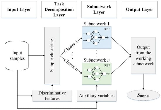
Figure 1.
The architecture of the proposed MNN.
- (1)
- The input layer is mainly responsible for importing the samples from the BSM1 model into the model.
- (2)
- The task decomposition layer decomposes the input samples into several clusters and allocates them to the respective modules. In this layer, we use a density-based clustering algorithm to decompose the input samples based on weather conditions using the most discriminative feature variables.
- (3)
- The subnetwork layer consists of several subnetworks, with the number of which determined by the number of clusters. The constructive RBF network based on error correction algorithm is utilized as the model for each subnetwork to predict BOD concentration. The input variables to the model are selected based on their correlation with SBOD,E.
- (4)
- The output layer obtains the final output by transporting the output of the working subnetwork.
The proposed scheme is introduced as follows in detail.
2.3. Task Decomposition in MNN
2.3.1. Feature Selection Method for Sample Clustering
To improve the results of sample clustering based on weather conditions, a filter-based feature selection method is used to select the most discriminative variables. The task decomposition layer could use these variables to divide the training samples into different clusters.
A discriminative index (DI) is defined to select the most discriminative features among groups from the input variables, which is measured by the ratio of between-group sum squares (BSS) to within-group sum squares (WSS). The DI value for each input variable is calculated according to
where Xp represents the normalized value of the pth sample (p = 1,…,p, and p is the number of samples) and Xk represents the vector of the variable in the group k (k = 1,…,K, and K is the number of groups). In this experiment, the group was defined by weather conditions, and K was set to 3 accordingly. mean() represents the average value and V is an indicator function. When the pth sample belongs to the group k, V equals to 1. Otherwise, V equals to 0.
Note that the discriminative variables should have a higher BSS value and a lower WSS value. Therefore, the variables which have DI values higher than a predefined threshold α are selected for task decomposition in MNN.
2.3.2. The Density-Based Clustering Algorithm
In the present study, the task decomposition layer adopted a density-based clustering algorithm [29] to divide the samples into several clusters using the selected discriminative features. It is based on the idea that cluster centers are characterized by a higher density than their neighbors and a relatively large distance from other samples with higher densities. For each sample, its local density is computed according to
where ρp is the local density of the pth sample and dp,i represents the distance between the pth and ith samples. dc is a cutoff distance and F is an indicator function. When dp,i − dc < 1, F equals 1. Otherwise, F equals 0. Note that the relative magnitude of ρp is used, and the choice of dc is thus robust for selecting the sample with a higher local density.
The relative distance is defined as the minimum distance between the sample and any other sample with a higher density. The relative distance of the pth sample is calculated as
For the sample with the highest density, its relative distance equals its maximum distance from any other samples. The samples with a higher local density and a higher relative distance could be recognized as the cluster centers. Therefore, an index γ is calculated for the pth sample according to
γp = δpρp
The samples with significantly higher γ values are identified as the cluster centers and the remaining samples are assigned to the same cluster that its nearest neighbors whose local densities are highest belong to. Subsequently, the samples from different clusters are input to respective subnetworks.
2.4. Design of the Subnetwork in MNN
2.4.1. Determination of Auxiliary Variables
In this paper, we adopt the mutual information (MI) to select auxiliary variables which are correlated with the effluent BOD. The MI between the mth input variable and the output variable is defined as
where Xm denotes the sample vector of the mth input variable and O represents the output vector. H(·) represents the entropy and is defined by Equation (7), taking Xm as an example.
where f(Xp,m) is a probability density function of the mth input variable estimated using the method of equal distance histogram. The joint entropy H(Xm,O) is defined as
where f(Xp,m,Op) denotes the joint probability density function of the mth input variable and the output variable, which is estimated using the method of equal distance histogram as well.
MI(Xm,O) = H(Xm) + H(O) − H(Xm,O)
The MI between each input variable and the output variable is calculated, and the variables which have higher MI values than a predefined threshold β are selected as auxiliary variables for each subnetwork. Note that the parameter β is set based on MI values for each input variable and with a moderate value to ensure the selection of auxiliary variables but without the loss of many features.
2.4.2. Construction of Models in Subnetworks
In the present study, the number of subnetworks in MNN equals the number of identified clusters. In each subnetwork, we adopt an RBF neural network as the model due to its strong capability for nonlinear system modeling, and the error correction algorithm [30] is utilized for constructing a compact structure automatically. We use the auxiliary variables as the input variables to the model. Training samples from different clusters are input to respective subnetworks. Let Xp = [Xp,1, Xp,2,…, Xp,M] denote the pth training sample in one subnetwork, where M is the number of auxiliary variables. The output of the hth hidden neuron in RBF neural network is calculated as
where ch and σh are the center and width of hth hidden neuron, respectively, and represents the Euclidean Norm. The network output for the pth sample is computed by
where ωh presents the connection weight between the hth hidden neuron (h = 1,2,…,H, with H the number of the hidden neuron) and network output and ω0 is the bias weight.
The procedure for error correction algorithm in each subnetwork is described as follows:
Step 1: Initialization. The number of hidden neurons is set to zero (H = 0). Set the parameters, including the maximal number of hidden neurons (Hm), the maximal iterations, and the desired training RMSE.
Step 2: Calculate the error between the desired and actual outputs for all training samples. The error for the pth sample is defined as
where Op and yp and are the desired and actual outputs for the pth sample. Find the maximal absolute error for all samples, and the samples with the maximal value is marked as pmax. Create a new hidden neuron by Equations (12)–(14)
and set H = H + 1.
ep = yp − Op
σH+1 = 1
ωH+1 = 1
Step 3: For the given RBF neural network, calculate Jacobian vector jp as
where
The quasi-Hessian matrix Q and the gradient vector g are obtained using Equations (19) and (20).
where ηp is the sub gradient vector. Then, update subnetwork parameters using Equation (21)
where I is the identity matrix and μ is the combination coefficient. t is the iteration step, and contains all the parameters to be updated in the subnetwork as
The training process is repeated until the desired training RMSE or the maximal number of iterations is reached.
Step 4: Calculate the training RMSE. If the training RMSE is no more than the desired training RMSE or the hidden neurons reaches Hm, the construction procedure ends. Otherwise, return to Step 2.
2.5. The Proposed Hybrid Scheme Based on MNN
The flowchart for the hybrid scheme proposed in the present study is illustrated in Figure 2. In brief, the DI value is first calculated for each input variables of training samples to select the discriminative variables for weather conditions. Then, the training samples are clustered using the density-based clustering algorithm, generating n clusters. Subsequently, an MNN consisting of n subnetworks is built, with the auxiliary variables selected based on MI as the inputs, and each subnetwork is self-constructed and trained using the error correction algorithm with the training samples from one cluster. When a testing sample comes in, it is allocated to one cluster, and the auxiliary variables of this testing sample are input to the corresponding subnetworks, with the output of this subnetwork as the predicted BOD concentration.
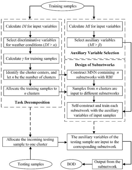
Figure 2.
The flowchart for the proposed hybrid scheme.
3. Results and Discussion
3.1. Experimental Setup
In the present study, 900 samples (500 samples from dry weather, 300 samples from rainy weather, and 100 samples from stormy weather) were collected from the BSM1 model. We randomly selected 80% of samples from each weather condition as training samples, and the remaining samples were used for testing. Each sample has 10 variables, with the effluent BOD concentration as the output variable and the remaining variables treated as the input variables. All the input and output variables were normalized to [0,1]. Twenty independent trails were conducted to evaluate the performance of the proposed scheme. The experiments were carried out in the MATLAB 9.0 environment running with an Inter(R) Core(TM) i7 CPU (2.00 GHz) and 8.00 GB RAM.
3.2. Discriminative Features for Sample Clustering
We set the threshold α to 3, and the variables with higher DI value than the threshold were selected as discriminative features. The average and standard deviation of DI value for each input variable over 20 independent trails were calculated, as listed in Table 1. We can see that three variables, QInf, SNH,E, and XTSS,E, have significantly higher DI values than other variables, indicating these variables are most discriminative among groups. To test the effectiveness of the feature selection method for sample clustering, the distributions of these three features are plotted in Figure 3. We can see that the distributions of these features are discriminative between different weather conditions, especially between the dry and other weather conditions.

Table 1.
The DI value for all input variables.
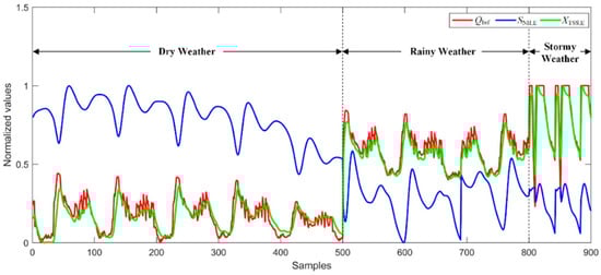
Figure 3.
Distributions of the three most discriminative features.
3.3. Sample Clustering
The training samples were then clustered by the density-based clustering algorithm using the most discriminative features. The cutoff distance dc was set to 0.1 in the present study. The index γ was calculated for each training sample and sorted in a descending order, and we plot it from one trail in Figure 4 as an example. Two samples exhibit significantly higher γ values than others, which are marked in red in the figure and thus considered as the cluster centers accordingly. The remaining training samples were assigned to the same cluster that its nearest neighbors whose local densities are highest belong to. For a testing sample, we calculated the distance between the testing sample and all training samples and assigned it to the same cluster as the nearest neighbors with the highest local density.
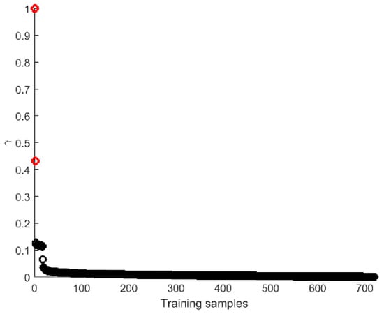
Figure 4.
The γ value in a descending order for all the training samples from one trail.
To figure out the effectiveness of the sample clustering, the average clustering results for training and testing samples over 20 independent trials are listed in Table 2. For the training samples, the first cluster consists of all samples from the dry weather and only few samples from the rainy and stormy weather, and the second cluster consists of samples only from rainy and stormy weather. The clustering accuracy is high for both training (99.92%) and testing samples (95.25%). These results demonstrate the effectiveness of the proposed scheme for sample clustering based on weather conditions. Since two clusters were obtained, the number of subnetworks in MNN was determined as 2. The samples after clustering were then input to the corresponding modules in MNN.
Table 2.
The average results for sample clustering.
3.4. Auxiliary Variables for BOD Prediction
The training samples were then used to select the auxiliary variables by calculating the MI between each input variable and the output variable. The average MI value for all input variables over 20 independent trials are listed in Table 3. In the present study, the threshold β was set to 6.5, and the variables which have a higher MI value than the threshold were selected. Accordingly, six variables, QInf, SNO,E, SNH,E, SCOD,Inf, SCOD,E, and XTSS,E, were mostly selected as the auxiliary variables for BOD prediction, which were the input variables for each subnetwork to train the model.
Table 3.
Values of MI for all input variables.
3.5. Results for BOD Prediction
For the training process of each subnetwork, the learning rate was set to 0.01, and the maximal number of iterations was set to 50. The training process ended when either the number of hidden neurons reached 10 or the training RMSE was not larger than 0.01. The root mean square error was used to evaluate the accuracy for BOD concentration prediction, which is defined as
where ep is the output error and p is the number of training samples.
Taking one trail as an example, we plot the training RMSE and the number of hidden neurons during training for each subnetwork in MNN in Figure 5. We can see that the training RMSE decreases with a sudden increase when the number of hidden neurons changes. With the increase of the hidden neurons, the training RMSE decreases and finally reaches the desired training RMSE, obtaining a compact network structure.
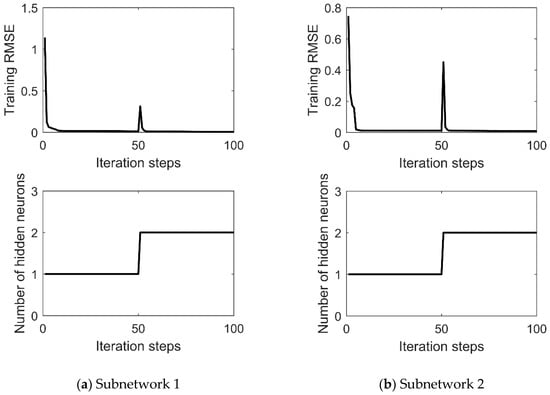
Figure 5.
The training RMSE and number of hidden neurons in each subnetwork in MNN during training.
After training, the testing sample was then presented to the corresponding subnetwork with its auxiliary variables input to the model, and the output was obtained from the model accordingly. Taking one trail as an example, Figure 6 shows the testing results and testing errors after anti-normalization, demonstrating the effectiveness of the proposed scheme.
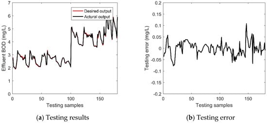
Figure 6.
The (a) testing results and (b) testing errors of the proposed scheme for BOD prediction.
To further evaluate the performance of the proposed scheme, the results were compared with other methods, including an MNN without consideration of the selection of discriminative features for sample clustering (AllClu-MNN), an MNN without the selection of auxiliary variables which uses all variables as the input variables for the subnetworks (AllIn-MNN), an MNN with the standard RBF neural network as the subnetworks (RBF-MNN), and one single RBF neural network with error correction algorithm (ErrCor-RBF). The training and testing RMSE, training time, and the number of hidden neurons in each subnetwork were used as the measurement for the performance evaluation, and the average results over 20 independent runs are listed in Table 4. We can see that the proposed scheme outperforms the other models in prediction accuracy, training time, and the compactness of the model structure.
Table 4.
Comparisons for average performance of different methods for BOD prediction in WWTP.
Comparison between the proposed MNN and AllClu-MNN demonstrates the performance improvement by the selection of discriminative features. In the proposed hybrid scheme, the discriminative features are used for sample clustering to improve the clustering accuracy, while AllClu-MNN uses all features for sample clustering, which may decrease the clustering accuracy and degenerate the model performance directly. Besides, comparing the proposed scheme with AllIn-MNN, the results show that the selection of the auxiliary variables can improve the generalization performance and shorten the training time, and the network structure is smaller as well. When we replace the subnetwork in the proposed MNN with a standard RBF (RBF-MNN), it directly causes a significant performance deterioration, demonstrating the superiority of using the ErrCor-RBF for subnetworks. Finally, the single ErrCor-RBF was tested, and the experimental results indicate that the modular structure can improve the generalization performance and significantly shorten the training time.
3.6. Performance Evaluation for Different Weather Conditions
To evaluate the performance of the proposed hybrid scheme on different weather conditions, we grouped the testing samples according to their labels for weather conditions, and the testing RMSE for each weather group was calculated (Table 5). We can see that the proposed MNN performs the best over other models for each weather condition. For the dry weather, the prediction accuracy is higher than other two weather conditions for all comparable models, the reason for which is that the key water parameters exhibit smaller fluctuations in the dry weather than other two weather conditions. Better prediction accuracy for rainy and stormy weather conditions is obtained by the proposed MNN and AllIn-MNN, indicating that using an individual module to model the data from rainy and stormy weather (all the training samples input to the second module are from the rainy and stormy weather, as shown in Table 2) provides a positive effect on the prediction accuracy for effluent BOD concentration. When using the single ErrCor-RBF to obtain a general model for data from different weather conditions, the prediction accuracy for effluent BOD concentration decreases for all the three weather conditions.
Table 5.
Testing RMSE of different methods for three weather groups.
4. Conclusions
We propose a novel hybrid scheme based on MNN combining the factor of weather condition to improve the BOD prediction. The effectiveness and superiority of the proposed scheme were evaluated on BSM1. Experimental results demonstrate that the proposed scheme outperforms the other models from the following aspects.
MNN is used as the model to predict effluent BOD with modules modeling using clustered samples based on weather conditions. Considering that different nonlinearities are observed for the key parameters in WWTP in different weather conditions, the input samples are clustered based on weather conditions and modeled by respective subnetworks. Experimental results demonstrate the superior performance of the proposed scheme on BOD prediction.
Discriminative features are selected to obtain a better clustering accuracy for samples from different weather conditions. These selected features are demonstrated to be discriminative among groups, and the accuracy for sample clustering is high to ensure a higher prediction accuracy for the effluent BOD.
Auxiliary variables which exhibit high correlations with the effluent BOD are selected as inputs to the model, which can improve the generalization performance, shorten the training time, and make the structure smaller.
The constructive RBF neural network with the error correction algorithm is used for each subnetwork in MNN. On the one hand, the structure of each subnetwork is determined automatically. On the other hand, the superior generalization performance and compact structure are provided by this model compared with the standard RBF neural network.
In summary, the proposed hybrid scheme based on MNN, in combination with weather conditions, improves the performance of the model, including the improved generalization ability, short training time, and compact structure. The BSM1 was used as a standard platform for the evaluation of the effectiveness of the proposed scheme, which provides a guidance for the soft measurement in the actual wastewater treatment process in the future.
Author Contributions
Conceptualization, W.L. and J.Z.; methodology, W.L.; software, J.Z.; validation, J.Z.; formal analysis, J.Z.; investigation, J.Z.; writing—original draft preparation, J.Z.; writing—review and editing, W.L.; visualization, J.Z.; supervision, W.L.; and funding acquisition, W.L. All authors have read and agreed to the published version of the manuscript.
Funding
This research was funded by the National Natural Science Foundation of China (61603009, 62021003, 61890930-5); the Natural Science Foundation of Beijing Municipality (4182007); the Beijing Municipal Education Commission Foundation (KM201910005023); and the Beijing Outstanding Young Scientist Program (BJJWZYJH01201910005020).
Conflicts of Interest
The authors declare no conflict of interest.
References
- Nordberg, M.; Templeton, D.M.; Andersen, O.; Duffus, J.H. Glossary of terms used in ecotoxicology (IUPAC Recommendations 2009). Pure Appl. Chem. 2009, 81, 829–970. [Google Scholar] [CrossRef]
- Spanjers, H.; Olsson, G.; Klapwijk, A. Determining influent short-term biochemical oxygen demand by combined respirometry and extimation. Water Sci. Technol. 1993, 28, 401–414. [Google Scholar] [CrossRef]
- Fulazzaky, M.A. Measurement of biochemical oxygen demand of the leachates. Environ. Monit. Assess. 2013, 185, 4721–4734. [Google Scholar] [CrossRef] [PubMed]
- Kwok, N.Y.; Dong, S.; Lo, W.; Wong, K.Y. An optical biosensor for multi-sample determination of biochemical oxygen demand (BOD). Sens. Actuators B Chem. 2005, 110, 289–298. [Google Scholar] [CrossRef]
- Niyomdecha, S.; Limbut, W.; Numnuam, A.; Asawatreratanakul, P.; Kanatharana, P.; Thavarungkul, P. A novel BOD biosensor based on entrapped activated sludge in a porous chitosan-albumin cryogel incorporated with graphene and methylene blue. Sens. Actuators B Chem. 2017, 241, 473–481. [Google Scholar] [CrossRef]
- Nakamura, H. Current status of water environment and their microbial biosensor techniques—Part II: Recent trends in microbial biosensor development. Anal. Bioanal. Chem. 2018, 410, 3967–3989. [Google Scholar] [CrossRef]
- Areerachakul, S.; Sanguansintukul, S. A Comparison between the Multiple Linear Regression Model and Neural Networks for Biochemical Oxygen Demand Estimations. In Proceedings of the 8th International Symposim on Natural Language Processing, Bangkok, Thailand, 20–22 October 2009; pp. 11–14. [Google Scholar] [CrossRef]
- Luo, L. Biochemical oxygen demand soft measurement based on LE-RVM. In Proceedings of the 2nd International Conference on Sustainable Development, Xi’an, China, 2–4 December 2017; Volume 94, pp. 164–167. [Google Scholar] [CrossRef]
- Yu, P.; Cao, J.; Jegatheesan, V.; Du, X. A real-time BOD estimation method in wastewater treatment process based on an optimized extreme learning machine. Appl. Sci. 2019, 9, 523. [Google Scholar] [CrossRef]
- Qiao, J.; Hu, Z.; Li, W. Soft measurement modeling based on chaos theory for biochemical oxygen demand (BOD). Water 2016, 8, 581. [Google Scholar] [CrossRef]
- Heddam, S.; Lamda, H.; Filali, S. Predicting effluent biochemical oxygen demand in a wastewater treatment plant using generalized regression neural network based approach: A comparative study. Environ. Process. 2016, 3, 153–165. [Google Scholar] [CrossRef]
- Dogan, E.; Sengorur, B.; Koklu, R. Modeling biological oxygen demand of the Melen River in Turkey using an artificial neural network technique. J. Environ. Manag. 2009, 90, 1229–1235. [Google Scholar] [CrossRef]
- Basant, N.; Gupta, S.; Malik, A.; Singh, K.P. Linear and nonlinear modeling for simultaneous prediction of dissolved oxygen and biochemical oxygen demand of the surface water—A case study. Chemom. Intell. Lab. Syst. 2010, 104, 172–180. [Google Scholar] [CrossRef]
- Khatri, N.; Khatri, K.K.; Sharma, A. Prediction of effluent quality in ICEAS-sequential batch reactor using feedforward artificial neural network. Water Sci. Technol. 2019, 80, 213–222. [Google Scholar] [CrossRef] [PubMed]
- Mirbagheri, S.A.; Bagheri, M.; Boudaghpour, S.; Ehteshami, M.; Bagheri, Z. Performance evaluation and modeling of a submerged membrane bioreactor treating combined municipal and industrial wastewater using radial basis function artificial neural networks. J. Environ. Health Sci. Eng. 2015, 13, 17. [Google Scholar] [CrossRef]
- Raheli, B.; Aalami, M.T.; El-Shafie, A.; Ghorbani, M.A.; Deo, R.C. Uncertainty assessment of the multilayer perceptron (MLP) neural network model with implementation of the novel hybrid MLP-FFA method for prediction of biochemical oxygen demand and dissolved oxygen: A case study of Langat River. Environ. Earth Sci. 2017, 76, 503. [Google Scholar] [CrossRef]
- Yan, J.; Xu, Z.; Yu, Y.; Xu, H.; Gao, K. Application of a hybrid optimized BP network model to estimatewater quality parameters of Beihai Lake in Beijing. Appl. Sci. 2019, 9, 1863. [Google Scholar] [CrossRef]
- Han, H.G.; Chen, Q.L.; Qiao, J.F. An efficient self-organizing RBF neural network for water quality prediction. Neural Netw. 2011, 24, 717–725. [Google Scholar] [CrossRef]
- Qiao, J.; Li, W.; Han, H. Soft computing of biochemical oxygen demand using an improved T—S fuzzy neural network. Chin. J. Chem. Eng. 2014, 22, 1254–1259. [Google Scholar] [CrossRef]
- Ahmed, A.A.M.; Shah, S.M.A. Application of adaptive neuro-fuzzy inference system (ANFIS) to estimate the biochemical oxygen demand (BOD) of Surma River. J. King Saud Univ. Eng. Sci. 2017, 29, 237–243. [Google Scholar] [CrossRef]
- Elkiran, G.; Nourani, V.; Abba, S.I. Multi-step ahead modelling of river water quality parameters using ensemble artificial intelligence-based approach. J. Hydrol. 2019, 577, 123962. [Google Scholar] [CrossRef]
- Lucas, F.S.; Therial, C.; Gonçalves, A.; Servais, P.; Rocher, V.; Mouchel, J.M. Variation of raw wastewater microbiological quality in dry and wet weather conditions. Environ. Sci. Pollut. Res. 2014, 21, 5318–5328. [Google Scholar] [CrossRef]
- Mines, R.O.; Lackey, L.W.; Behrend, G.H. The impact of rainfall on flows and loadings at Georgia’s wastewater treatment plants. Water Air Soil Pollut. 2007, 179, 135–157. [Google Scholar] [CrossRef]
- Alex, J.; Benedetti, L.; Copp, J.; Gernaey, K.V.; Jeppsson, U.; Nopens, I.; Pons, M.N.; Steyer, J.P.; Vanrolleghem, P.A. Benchmark Simulation Model no. 1 (BSM1); Lund University: Lund, Sweden, 2008; pp. 1–62. [Google Scholar]
- Rastegar, S.; Araújo, R.; Mendes, J. Online identification of Takagi-Sugeno fuzzy models based on self-adaptive hierarchical particle swarm optimization. Appl. Math. Model. 2017, 45, 606–620. [Google Scholar] [CrossRef]
- Li, Z.; Yan, X. Complex dynamic process monitoring method based on slow feature analysis model of multi-subspace partitioning. ISA Trans. 2019, 95, 68–81. [Google Scholar] [CrossRef] [PubMed]
- Li, D.; Huang, D.; Yu, G.; Liu, Y. Learning adaptive semi-supervised multi-output soft-sensors with co-training of heterogeneous models. IEEE Access 2020, 8, 46493–46504. [Google Scholar] [CrossRef]
- Modelling & Integrated Assessment. Available online: http://www.benchmarkWWTP.org/ (accessed on 15 June 2020).
- Rodriguez, A.; Laio, A. Clustering by fast search and find of density peaks. Science 2014, 344, 1492–1496. [Google Scholar] [CrossRef]
- Yu, H.; Reiner, P.D.; Xie, T.; Bartczak, T.; Wilamowski, B.M. An incremental design of radial basis function networks. IEEE Trans. Neural Netw. Learn. Syst. 2014, 25, 1793–1803. [Google Scholar] [CrossRef]


Publisher’s Note: MDPI stays neutral with regard to jurisdictional claims in published maps and institutional affiliations. |
© 2020 by the authors. Licensee MDPI, Basel, Switzerland. This article is an open access article distributed under the terms and conditions of the Creative Commons Attribution (CC BY) license (http://creativecommons.org/licenses/by/4.0/).