Optimal Robot Motion for Accelerated Life Testing of a 6-DoF Industrial Robot

Featured Application

The motion optimization method proposed in this study can be applied to the design of a test mode for performing system-level accelerated life tests of robot driving parts such as servo motors and gearboxes.

Abstract

In order to verify the reliability of drive components for industrial robots, component-level life tests must be accompanied by a system-level life test using actual robots in which predefined robot motions are repeated throughout the test. To properly verify the durability of drive components through a system-level life test, it is important to design test modes so that the required test time is the same for all joint drive components of the robot, and it is necessary to design test modes with a high acceleration factor so as to shorten the required test time as much as possible. To solve this problem, the present research proposes a method for designing robot motions that makes the accelerated life test time for all the drive components of the robot equal. In particular, we solve a dynamic based motion optimization problem for an industrial 6-DoF (degrees-of-freedom) robot that minimizes the AM-GM (arithmetic mean to geometric mean) ratio of the acceleration factors of each joint. The results show that $C^2$-continuous test modes with the same acceleration factor, which is inversely proportional to the cycle time of the robot motion, can be derived.

1. Introduction

Industrial 6-DoF (degrees-of-freedom) robots are widely used for the automation of various manufacturing processes, such as welding, assembly, painting, inspection, etc. As the demand for industrial 6-DoF robots continues to increase, robot manufacturers are correspondingly researching the development and performance improvement of robots to meet the requirements of various applications.

It is imperative to ensure the performance and reliability of robot drive components including servo motors and gearboxes in improving the accuracy and responsiveness of industrial robots. In particular, a high-precision gearbox with little backlash and high reduction ratio is a key component which determines the accuracy and performance of a robot, and since the weight of the gearbox is directly related to the payload of robots, a small size, light weight, and high torque density design is required. Therefore, high-precision gearboxes, such as harmonic drives [1] and planocentric type 2-stage precision gearboxes [2], are applied to many industrial robots requiring high accuracy and responsiveness. High-precision drive components occupy the highest proportion in the manufacturing cost of robots, and it is essential to ensure stable performance and reliability because they can cause downtime and accidents of the automated process in the event of a failure.

In the field of reliability application, the most commonly used test methods for reliability qualification are zero-failure acceptance tests since they require fewer test samples and less test time compared to other test methods that guarantee the same reliability with a given confidence level [3]. To verify the reliability of drive components for industrial multi-joint robots, component-level life tests must be accompanied by a system-level life test in which the drive components are mounted on an actual robot, and predefined test modes are repeated to verify the durability.

A zero-failure acceptance test concept can be applied to calculate the test time for the guaranteed life of each joint part in system-level life test, and an acceleration test is designed by comparing the test load with the load in guaranteed conditions. The load applied to the drive components of each joint of the robot will depend on the payload and the motion profile. This can also result in differences in the degree of damage to the drive components, which results in a difference in the required test time.

As a consequence, the overall zero failure test time is determined by the longest test time among the required test times of each joint of the robot. If the variation of the required test time for each joint is large, the parts tested in excess of the required time have higher probability of failure, necessitating the repair or replacement of damaged components, and thus requiring more time and cost for the test. There is a method to stop the motion of the joint after the test time has been completed, but it can be cumbersome for the tester such as monitoring the time when the test time for each axis is completed and operating in a new test mode, etc. especially when the test scale is large.

Therefore, one of the ideas to verify the durable life of a robot drive component through system-level accelerated life testing is to design a test mode with the same zero failure test time for all the joint drive components. At the same time, it is necessary to design the test with a high acceleration factor to reduce the test time required to verify the durable life. For this purpose, the industry has been using robot simulation software to design test modes based on experience and intuition of engineers and trial and error. Therefore, it took a lot of time to derive robot motions that match the test times for the components of the individual joints equally, and there was a limit in the accuracy.

Motivated by the above observation, the goal of this study is to develop a numerical method for designing robot motions for system-level life test of drive components of robot.

In order to achieve the research goal, this study drew the following results: (1) A dynamic based optimization problem was formulated in which motion profiles defined over a fixed cycle time are used as optimization variables and the AM-GM ratio of the acceleration factors of each joint is used as an objective function. (2) For a given initial and final pose of a robot, a global minimum solution that that makes the accelerated life test times for the drive components of all joints of a robot equal was derived. (3) Using the kinematics and dynamics parameters of an actual 6-DoF industrial robot, a global optimal solution was obtained for various cycle times and it was confirmed that the acceleration factor is inversely proportional to the cycle time.

From the above results, it was possible to design robot motions which have the following useful properties for system-level life test: equal test time for the drive components of all joints of a robot, smooth joint displacement so that the required joint torque is continuous, and high acceleration factor to shorten the required test time.

Robotic motion optimizations for various robots have been studied to date [4,5,6,7,8,9,10], but most have focused on optimizing efficiency and performance, such as minimizing energy consumption or shortening cycle time to perform a particular task. What distinguishes the present study from past works relating the robot motion optimization is that the present study is a result of studies on motion optimization to ensure that the load applied to each drive component is evenly distributed.

In refs. [4,5,6,7,8], motion optimization problems are established with robot dynamics based on Lie group. A recursive algorithm to obtain the analytic gradient that can be used to perform motion optimization is presented, and the displacement of the robot joint was parameterized with a B-spline curve to convert the problem into a finite-dimensional constrained optimization problem. In Martin et al. [6] and Bobrow et al. [7], minimum effort optimal motions for various open chain manipulators are examined, In Wang el al. [8], the result of applying motion optimization for maximizing payload to the industrial robot PUMA is presented. The result of applying motion optimization technique to the hydraulic excavator and the bipedal humanoid robot are given in [9] and [10], respectively. The efficient generation of the natural robot motion based on dynamics-based optimization and principal component analysis is presented in [11].

Studies on the reliability and lifetime of robots have been conducted mainly on a component-by-component basis, and there have been few studies to systematically design the life test at system-level. In this paper, it was attempted to design robot motions for the accelerated life test of drive components at system level by applying a robot motion optimization technique.

Studies on the reliability and lifetime of precision gearboxes used in robots are presented in [12,13,14] and work on servo motors are summarized in [15]. In ref. [16], an accelerated life test was performed on individual components to calculate the reliability of the entire system from the reliability of each component of the robot, and the average lifetime of the system was estimated from the results. In ref. [17], a study on motion optimization to increase the service life of the robot gearbox was conducted.

This paper is configured as follows. In Section 2, modeling for the dynamic analysis of industrial 6-DoF is presented. Section 3 introduces a concept of a zero failure life test and an acceleration factor in relation to an accelerated life test for drive components of an industrial 6-DoF robot. Section 4 establishes a motion optimization problem that can verify the lifetime of all the drive components within the zero failure test time by matching the acceleration factor of each robot joint equally. Section 5 shows the results of performing the motion profile optimization to the actual 6-DoF industrial robot. Section 6 summarizes the main results of the study as a conclusion.

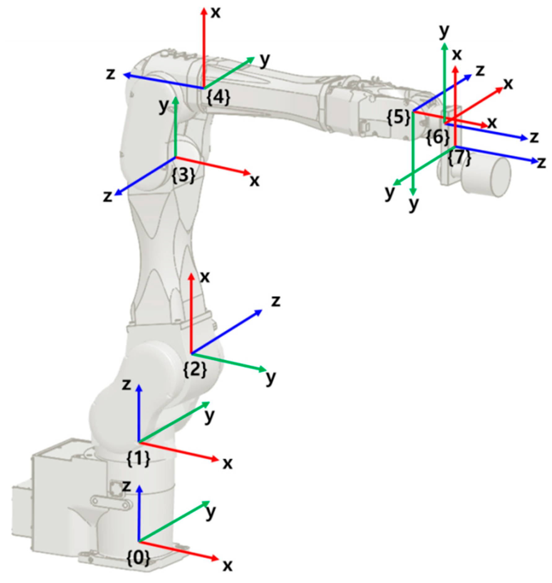
2. Dynamic Modeling of the Robot

Figure 1 represents a 6-DoF industrial robot that is the subject of this study. The robot link is numbered from 1 to 6 and the body-fixed coordinate frames are attached to each link as in the figure. The coordinate frame 0 is a space fixed frame of reference and coordinate frame 7 is attached to an object fixed to the link 6.

The equation of motion for such a serial robot can be described with a recursive Newton-Euler equation. The Newton-Euler equation can be expressed using Lie algebraic expressions as shown in Equations (1)–(6) [18,19].

Given arbitrary value of joint angle $q_i$, speed ${\dot{q}}_i$ and acceleration ${\ddot{q}}_i$, the inverse dynamics algorithm given in Equations (1)–(6) calculates the joint torque ${\tau }_i$. The algorithm starts by initializing the generalized velocity of the space fixed frame and the generalized forces exerted on the end-effector as in Equation (1). The load torque by gravity is reflected in the joint torque by initializing the generalized acceleration of the space fixed frame to the acceleration due to gravity.

In the outward recursion phase, the coordinate transformation matrices between the adjacent links $T_{i-1,i}$ are calculated for the joint angle as Equation (2), where $M_i$ are the coordinate transformation matrices in home position. Then the generalized velocity $V_i$ and their time derivatives ${\dot{V}}_i$ are calculated recursively in the order from the base frame to the end effector as Equations (3) and (4).

In the inward recursion phase, the generalized forces $F_i$ for each link are obtained recursively by solving the Equation (5) in the order from the end effector to the base frame. The joint torque is then calculated from the joint motion direction component of the generalized force as Equation (6).

The derivation of the algorithm including the mathematical definition of the adjoint operators $A{d}_T$ and $a{d}_V$ can be found in the original paper [18,19].

Initialization:

$$V_0=0, {\dot{V}}_0={\left[0,0,0,0,0,g\right]}^T, F_{n+1}=0.$$

(1)

Outward recursion (from i = 1 to i = 6):

$$T_{i-1,i}=M_i{e}^{S_i{q}_i},$$

(2)

$$V_i=A{d}_{T_{i-1,i}^{-1}}{V}_{i-1}+S_i{\dot{q}}_i,$$

(3)

$${\dot{V}}_i=A{d}_{T_{i-1,i}^{-1}}{\dot{V}}_{i-1}+a{d}_{V_i}{S}_i{\dot{q}}_i+S_i{\ddot{q}}_i.$$

(4)

Inward recursion (from i = 6 to i = 1):

$$F_i=A{d}_{T_{i-1,i}^{-1}}^{*}{F}_{i+1}+J_i{\dot{V}}_i-a{d}_{V_i}^{*}{J}_i{V}_i,$$

(5)

$${\tau }_i=S_i^T{F}_i.$$

(6)

3. Accelerated Life Testing of Robot

Among the drive components of the high-precision robot dealt with in this study, the high-precision gearbox is the most prone to deterioration due to friction and wear, and thus can be seen as a component that has the greatest influence on the durability of the robot. The life of the high-precision gearbox is determined by the life of the bearing supporting the input-side rotary shaft. Therefore, the zero failure test time $T_n$ to verify the durability of the gearbox is derived from Equation (7) [3].

$$T_n=B_{100p}{\left[\frac{\ln \left(1-CL\right)}{n·\ln \left(1-p\right)}\right]}^{\frac{1}{\beta }}.$$

(7)

where B_100p is the guaranteed lifetime according to the conditions of use, $CL$ is the required confidence level, $n$ is the number of samples, $p$ is the cumulative probability of failure, and $\beta$ is the shape parameter.

The guaranteed lifetime for the rated use conditions of the gearbox is usually given by component-level life test results from the manufacturer. The precision gearbox used in a variable load environment can then be guaranteed in service life only when used within the permissible torque presented by the manufacturer, which is related to the service life of the bearings of the precision gearbox components.

Ball bearings (e.g., in harmonic gearboxes) or roller bearings (e.g., in planocentric type 2-stage precision gearboxes) are used in precision gearboxes depending on the load class and characteristics [1,2]. Bearings have a well-established theory and wealth of verifications, and the lifetimes of precision reducers are also calculated according to this theory.

First, from the load torque $\tau$ and speed $\omega$ of the gearbox over a fixed cycle time of $t_f$, equivalent load torque ${\tau }_{eq}$ and equivalent speed ${\omega }_{eq}$ are defined as Equations (8) and (9). Here, the index $\mathsf{\alpha }$ is determined by the type of bearings used: $\mathsf{\alpha }=3$ when ball bearings are used and $\mathsf{\alpha }=10/3$ when roller bearings are used as input rotary parts [20].

$${\tau }_{eq}={\left(\frac{{\int }_0^{t_f}\left|\omega \right|{\left|\tau \right|}^{\mathsf{\alpha }}dt}{{\int }_0^{t_f}\left|\omega \right|dt}\right)}^{1/\mathsf{\alpha }},$$

(8)

$${\omega }_{eq}=\frac{1}{t_f}{\int }_0^{t_f}\left|\omega \right|dt.$$

(9)

Then, the acceleration factor $AF$ of the motion profile having the equivalent load torque ${\tau }_{eq}$ and the equivalent speed ${\omega }_{eq}$ based on the rated torque ${\tau }_{rate}$ and the rated speed ${\omega }_{rate}$ of the robot’s precision gearbox can be defined as the Equation (10).

Consequently, according to the definition of zero failure test time $T_n$ and the acceleration factor, the accelerated life test time $T_{accel}$ can be calculated as in Equation (11) [21].

$$AF={\left(\frac{{\tau }_{eq}}{{\tau }_{rate}}\right)}^{\mathsf{\alpha }}·\left(\frac{{\omega }_{eq}}{{\omega }_{rate}}\right)=\frac{1}{t_f}\frac{{\int }_0^{t_f}\left|\omega \right|{\left|\tau \right|}^{\mathsf{\alpha }}dt}{{\tau }_{rated}^m·{\omega }_{rated}},$$

(10)

$$T_{accel}=\frac{T_n}{AF}.$$

(11)

The purpose of the present study is to design a test mode in which the system-level life test of precision gearboxes for robots is completed in the shortest time possible, and the durability of all gearboxes can be verified in one test without replacing samples during the life test.

In other words, the goal is to design a motion profile that allows the accelerated life test time $T_{accel}$ required by the precision gearbox mounted to each joint of the robot to be the same, and makes $T_{accel}$ as small as possible.

4. Formulation of Optimization Problem

Without loss of generality, and under the assumption that the zero failure life test time $T_n$ required for the gearboxes used in each joint of the robot are the same, all acceleration factors must be the same to ensure that the acceleration life test time $T_{accel}$ is the same for each joint.

All of the acceleration factors of the drive components derived from Equations (8)–(10) for each joint of the robot have non-negative values, so an inequality as shown in Equation (12) holds for their arithmetic and geometric means. Here, the degrees of freedom of robot is designated by $N$ to make the expression more general. The necessary and sufficient condition to make them equal is that acceleration factors for all drive components have the same value.

$$\frac{A{F}_1+A{F}_2+\cdots +A{F}_N}{\mathrm{N}}\ge \sqrt[\mathrm{N}]{A{F}_1·A{F}_2\cdots A{F}_N}.$$

(12)

Therefore, in this study, a function J, which represents the ratio of the arithmetic mean of the acceleration factors to their geometric mean, is defined as Equation (13), and its logarithmic value as in Equation (14) is defined as the cost function of the optimization problem. This ensures that the acceleration factor of each drive component converges to the same value when the global minimum is reached, where the cost function is zero as in Equation (15).

$$\mathrm{J}=\frac{1}{\mathrm{N}}\sum _{\mathrm{i}=1}^{\mathrm{N}}A{F}_i/{(\prod _{\mathrm{i}=1}^{\mathrm{N}}A{F}_i)}^{\frac{1}{\mathrm{N}}}\ge 1,$$

(13)

$$\log \mathrm{J}=\log \frac{1}{\mathrm{N}}{\displaystyle \sum }_{\mathrm{i}=1}^{\mathrm{N}}A{F}_i-\frac{1}{\mathrm{N}}{\displaystyle \sum }_{\mathrm{i}=1}^{\mathrm{N}}\log A{F}_i\ge 0,$$

(14)

$$\log \mathrm{J}=0\leftrightarrow A{F}_1=A{F}_2=\cdots =A{F}_N.$$

(15)

As a result, the problem of obtaining a motion profile in which all acceleration factor are the same during the predefined cycle time $t_f$ can be defined as a constrained optimization problem that minimizes the logarithm of AM-GM ratio (Equation (16)) while satisfying constraints on torque ${\tau }_i\left(t\right)$, speed ${\dot{q}}_i\left(t\right)$, and displacement $q_i\left(t\right)$ of the robot drive components as in Equations (18)–(22). Here, the Equation (17) is the dynamic equation which is solved from the Equations (1)–(6) and ${\tau }_i^{max}$, ${\dot{q}}_i^{max}$ is limit on joint torque and speed, respectively. The lower and upper bound of each joint displacement is designated by $q_i^{min}$ and $q_i^{max},$ and the initial and final value of the joint angles during the specific cycle time $t_f$ is $q_0$ and $q_f$.

$$\underset{q\left(t\right)}{\min }(\log \frac{1}{N}\sum _{i=1}^{N}A{F}_i-\frac{1}{N}\sum _{i=1}^N\log A{F}_i),$$

(16)

$$\mathrm{M}\left(q\right)\ddot{q}+C\left(q, \dot{q}\right)\dot{q}+G\left(q\right)=\tau ,$$

(17)

$$-{\tau }_i^{max}\le {\tau }_i\left(t\right)\le {\tau }_i^{max},$$

(18)

$$-{\dot{q}}_i^{max}\le {\dot{q}}_i\left(t\right)\le {\dot{q}}_i^{max},$$

(19)

$$q_i^{min}\le q_i\left(t\right)\le q_i^{max},$$

(20)

$$q\left(0\right)=q_0, q\left(t_f\right)=q_f,$$

(21)

$$\dot{q}\left(0\right)=0, \dot{q}\left(t_f\right)=0.$$

(22)

Since the motion profile that causes the acceleration factor of the gearboxes of each joint to be the same is not unique the above optimization problem may contain multiple global minimum. Therefore, the solution of the above constrained optimization problem can converge to different global optimal solutions depending on the initial setting values of the optimization variable. Moreover, according to the definition of the acceleration factor in Equation (10), the acceleration factor can be maximized by making the drive torque ${\tau }_i\left(t\right)$ of the individual gearbox have two states of $\pm {\tau }_i^{max}$.

However, the drive torque ${\tau }_i\left(t\right)$ obtained through such two state controls can cause chattering. In addition, the stepwise rapid change of drive torque can stimulate unmodeled dynamics such as the stiffness of the links and joints of the robot. This can lead to oscillatory robot motion, and the acceleration factor will also vary as the robot may not move as intended.

Therefore, in this study, the displacement of the robot drive component $q\left(t\right)$, which is an optimization variable, is limited to have a sufficiently smooth profile that is continuous up to the second derivative. This ensures the resulting load torque ${\tau }_i\left(t\right)$ of the robot drive component is continuous function of the time.

To this end, by parametrizing the displacement of each joint using B-spline as in Equation (23), we converted the constrained optimization problem defined in Equations (16)–(22) into a finite-dimensional constrained optimization problem [4,5,6,7,8].

$$q_i\left(t\right)={\displaystyle \sum }_{j=0}^{m-1}{p}_i^j{B}_{j,k}\left(t\right),\hspace{1em}\hspace{1em}i=1,\dots , N.$$

(23)

where $k$ is the order of the B-spline, $m$ is the number of control points, $p_i^j$ is the $j$-th control point for interpolation of the displacement of the $i$-th joint, and $B_{j,k}\left(t\right)$ is the B-spline basis function.

According to the definition of B-spline curve, the knot sequence was defined as a sequence $\mathsf{\delta }$ of $m+k+1$ elements, and all elements in the sequence except for $k+1$ overlapped elements at the beginning and end increase at equal intervals as the Equation (24)

$$\mathsf{\delta }=\left[\stackrel{k+1}{\overbrace{0, \dots ,0}}, \frac{t_f}{m-k}, \frac{2t_f}{m-k}, \dots , \frac{\left(m-k-1\right)t_f}{m-k}, \stackrel{k+1}{\overbrace{t_f, \dots ,t_f}}\right].$$

(24)

When the displacement of the robot drive component is expressed using B-spline, the constraint Equations (21) and (22) on the displacement and speed of the optimization problem can be satisfied by setting four points of the B-spline control points as in Equations (25) and (26) [8].

$$p_i^0=p_i^1=q_i\left(0\right), i=1,\dots ,N,$$

(25)

$$p_i^{m-2}=p_i^{m-1}=q_i\left(t_f\right),i=1,\dots ,N.$$

(26)

Therefore, the optimal variable $x$ is defined as in Equation (27) by augmenting $m-4$ B-spline control points that describes the displacement of the drive components for each joint of the robot.

$$x=\left[p_i^j\right]={\left[p_1^2, \dots , p_1^{m-3}, \dots , p_N^2, \dots , p_N^{m-3}\right]}^T\in R^{N\left(m-4\right)}.$$

(27)

To summarize the above results, the constrained optimization problem of Equations (16)–(22) can be expressed as a finite-dimensional optimization problem of Equations (28)–(30) for the optimization variable $x$.

$$\underset{x}{\min }(\log \frac{1}{N}\sum _{i=1}^{N}A{F}_i-\frac{1}{N}\sum _{i=1}^N\log A{F}_i+{\int }_0^{t_f}{\rho }^T\rho dt),$$

(28)

$$-c\le Ax+b\le c,$$

(29)

$$\underset{\_}{x}\le x\le \overline{x}.$$

(30)

The linear inequality in Equation (29) represents the constraint in Equation (19) for the rotational speed of each joint in terms of the optimization variable $x$, and the inequality in Equation (30) represents the constraint condition in Equation (20) for the displacement of each joint.

The matrix $A$ of Equation (29) is a block diagonal matrix and it is defined as a matrix having submatrix $A_i\in {\mathrm{R}}^{\left(\mathrm{m}-3\right)\times \left(\mathrm{m}-4\right)}$ as elements. Submatrix $A_i$ is a band diagonal matrix and is defined as Equation (31).

$$A=diag\left\{A_1,\dots , A_N\right\}, A_i\left(j,k\right)=\{\begin{array}{cc}1& if j=k,\\ -1& if j=k+1,\\ 0& otherwise.\end{array}$$

(31)

The vector $b$ in Equation (29) is an augmentation of vector $b_i\in R^{\left(m-3\right)}$, defined as in Equation (32). Then the deviation between adjacent control points of the B-spline was calculated by linear transformation of $Ax+b$.

$$b={\left[b_1^T, \dots , b_N^T\right]}^T,b_i={\left[-q_i\left(0\right), 0,\dots ,0,q_i\left(t_f\right)\right]}^T.$$

(32)

The vector $c$ in the Equation (29) is an augmentation of vector $c_i\in R^{\left(m-3\right)}$, defined as in Equation (33), and the vector $c_i$ is derived by removing the first two and the last two elements from the knot sequence $\mathsf{\delta }$ of Equation (24) and using the $k$-th difference of thus formed sequence where $k$ is the B-spline order.

$$c={\left[c_1^T, \dots , c_N^T\right]}^T, c_i=\frac{{\dot{q}}_i^{max}}{k}{\left[{\mathsf{\delta }}_{k+2}-{\mathsf{\delta }}_2, \dots , {\mathsf{\delta }}_{k+m-2}-{\mathsf{\delta }}_{m-2}\right]}^T.$$

(33)

The vector ${\underset{\_}{x}}_i, {\overline{x}}_i\in R^{\left(m-3\right)}$ is defined by Equations (34) and (35) and includes parameters for the minimum and maximum angles of the individual joints.

$$\underset{\_}{x}={\left[{\underset{\_}{x}}_1^T, \dots , {\underset{\_}{x}}_N^T\right]}^T, {\underset{\_}{x}}_i={\left[q_i^{min},\dots ,q_i^{min}\right]}^T,$$

(34)

$$\overline{x}={\left[{\overline{x}}_1^T, \dots , {\overline{x}}_N^T\right]}^T,{\overline{x}}_i={\left[q_i^{max},\dots ,q_i^{max}\right]}^T.$$

(35)

The optimization tool utilized in this paper (python Scipy.optimize module) requires the objective function and the function for the constraint are entered separately, so if the constraint Equation (18) for the driving torque of each joint is reflected as a hard constraint, the dynamic equation must be evaluated in duplicate. In addition, it is necessary to implement a function with dimension as high as the number of sampling points to check whether the torque constraint is satisfied for each evaluation point. As a result, it may take longer computation time to solve the optimization problem. Therefore, we decide to reflect the constraint Equation (18) as a soft constraint by adding the quadratic penalty function of the vector $\rho$ defined in Equation (36) to the objective function.

As a result, a constrained optimization problem with linear constraints on the control points of the B-Spline curve, which is an optimization variable, was established.

$$\rho ={\left[{\rho }_1^T, \dots , {\rho }_N^T\right]}^T, {\rho }_i={\left[\max \left(0, {\tau }_i-{\tau }_i^{max}\right), \max \left(0, {\tau }_i^{min}-{\tau }_i\right)\right]}^T\in R^2.$$

(36)

5. Optimization Result

5.1. Problem Data

In order to analyze the dynamics of the 6-DoF industrial robot with the above algorithm, kinematic parameters such as the coordinate transformation matrices at home position $M_i=\left[\begin{array}{cc}{R}_i& p_i\\ 0& 1\end{array}\right]$ and the screw vectors $S_i$ are necessary that appears in Equation (2). Here, $R_i$ represents a rotation matrix to convert a 3D spatial vector represented in the $i$-th link coordinates into the $i-1$-th link coordinates. $p_i$ is a vector in which the origin of the $i$-th link coordinates is represented in the $i-1$-th link coordinates. $S_i$ represents a screw vector to express the degree of freedom of the $i$-th joint.

Table 1. Coordinate transformation matrices and screw vectors for the 6-DoF robot.

$\mathbf{Index} \left(\mathit{i}\right)$	$\mathbf{Rotation} \left({\mathit{R}}_{\mathit{i}}\right)$	$\mathbf{Translation} \left({\mathit{p}}_{\mathit{i}}\right)$	$\mathbf{Screw} \mathbf{Vector} \left({\mathit{S}}_{\mathit{i}}\right)$
1	$\lceil \begin{array}{ccc}1& 0& 0\\ 0& 1& 0\\ 0& 0& 1\end{array}\rceil$	$\lceil \begin{array}{c}0\\ 0\\ 0.108\end{array}\rceil$	$\left[\begin{array}{c}0\\ 0\\ 1\\ 0\\ 0\\ 0\end{array}\right]$
2	$\lceil \begin{array}{ccc}0& 1& 0\\ 0& 0& 1\\ 1& 0& 0\end{array}\rceil$	$\lceil \begin{array}{c}0.200\\ 0.177\\ 0.250\end{array}\rceil$
3	$\lceil \begin{array}{ccc}0& 1& 0\\ 1& 0& 0\\ 0& 0& -1\end{array}\rceil$	$\lceil \begin{array}{c}0.560\\ 0\\ -0.177\end{array}\rceil$
4	$\lceil \begin{array}{ccc}0& 0& -1\\ 1& 0& 0\\ 0& -1& 0\end{array}\rceil$	$\lceil \begin{array}{c}0.178\\ 0.140\\ 0\end{array}\rceil$
5	$\lceil \begin{array}{ccc}0& -1& 0\\ 0& 0& 1\\ -1& 0& 0\end{array}\rceil$	$\lceil \begin{array}{c}0\\ 0\\ -0.472\end{array}\rceil$
6	$\lceil \begin{array}{ccc}0& 0& 1\\ 0& -1& 0\\ 1& 0& 0\end{array}\rceil$	$\lceil \begin{array}{c}0.063\\ 0\\ 0\end{array}\rceil$
7	$\lceil \begin{array}{ccc}0& -1& 0\\ 1& 0& 0\\ 0& 0& 1\end{array}\rceil$	$\lceil \begin{array}{c}0\\ -0.058\\ 0.016\end{array}\rceil$	-

shows the kinematic parameters for the industrial robot used in this study.

In the dynamics analysis with inward recursion, an inertial parameter expressed as

$$J_i=\left[\begin{array}{cc}{I}_i-m_i{\left[r_i\right]}^2& m_i\left[r_i\right]\\ -m_i\left[r_i\right]& m_i·1\end{array}\right]$$

is required. Here, $I_i$ is the rotational inertia at the center of gravity of the $i$-th link, $r_i$ is the position of the center of gravity of the $i$-th link expressed in the $i$-th link coordinates, and $m_i$ is the mass of the $\mathrm{i}$-th link.

Table 2. Inertial parameters for the 6-DoF robot.

Link	${\mathit{I}}_{\mathit{x}\mathit{x}} \left(kg{m}^2\right)$	${\mathit{I}}_{\mathit{x}\mathit{y}} \left(kg{m}^2\right)$	${\mathit{I}}_{\mathit{x}\mathit{z}} \left(kg{m}^2\right)$	${\mathit{I}}_{\mathit{y}\mathit{y}} \left(kg{m}^2\right)$	${\mathit{I}}_{\mathit{y}\mathit{z}} \left(kg{m}^2\right)$	${\mathit{I}}_{\mathit{z}\mathit{z}} \left(kg{m}^2\right)$
1	1.035 × 100	1.615 × 10−2	−4.038 × 10−1	1.749 × 100	6.423 × 10−3	1.704 × 100
2	6.968 × 10−2	4.534 × 10−3	3.603 × 10−2	1.064 × 100	−3.916 × 10−3	1.095 × 100
3	2.853 × 10−2	−1.836 × 10−3	−3.915 × 10−3	3.356 × 10−2	−5.231 × 10−3	3.721 × 10−2
4	2.602 × 10−1	−1.805 × 10−7	2.179 × 10−4	2.563 × 10−1	−2.879 × 10−4	2.102 × 10−2
5	1.250 × 10−3	1.078 × 10−5	4.926 × 10−8	1.699 × 10−3	0 × 100	2.103 × 10−3
6	2.935 × 10−4	0 × 100	0 × 100	2.935 × 10−4	0 × 100	4.615 × 10−4
7	1.577 × 10−2	0 × 100	5.550 × 10−3	2.324 × 10−2	0 × 100	1.279 × 10−2
Link	${\mathit{r}}_{\mathit{x}} \left(m\right)$	${\mathit{r}}_{\mathit{y}} \left(m\right)$	${\mathit{r}}_{\mathit{z}} \left(m\right)$	$m \left(kg\right)$
1	4.969 × 10−2	2.218 × 10−2	1.757 × 10−1	7.147 × 101
2	2.675 × 10−1	1.557 × 10−2	−3.977 × 10−3	2.468 × 101
3	2.386 × 10−2	1.063 × 10−1	1.526 × 10−3	2.592 × 100
4	−5.593 × 10−5	4.071 × 10−4	−2.620 × 10−1	7.889 × 100
5	1.490 × 10−2	−2.619 × 10−4	3.226 × 10−6	1.029 × 100
6	0 × 100	0 × 100	−1.775 × 10−2	4.183 × 10−1
7	−4.213 × 10−2	0 × 100	6.046 × 10−2	5.785 × 100

is the inertial parameters for the industrial robot used in this study. The inertial matrix $J_7$ for the object fixed to link 6 was converted into a representation of the coordinates of link 6 as

$$A{d}_{T_{6,7}^{-1}}^{*}{J}_{w}A{d}_{T_{6,7}^{-1}}$$

and the analysis was performed by summing it up to the rotational inertia of link 6.

The limit on displacement, speed and torque of each joint is given in

Table 3. Limit on joint displacement, speed and torque.

Joint	${\mathit{q}}_{\mathit{m}\mathit{i}\mathit{n}} (°)$	${\mathit{q}}_{\mathit{m}\mathit{a}\mathit{x}} (°)$	${\dot{\mathit{q}}}_{\mathit{m}\mathit{a}\mathit{x}} \left(\mathbf{r}\mathbf{p}\mathbf{m}\right)$	${\dot{\mathit{q}}}_{\mathit{r}\mathit{a}\mathit{t}\mathit{e}} \left(\mathbf{r}\mathbf{p}\mathbf{m}\right)$	${\mathit{\tau }}_{\mathit{m}\mathit{a}\mathit{x}} \left(\mathbf{N}\mathbf{m}\right)$
1	−172	172	38	15	412
2	−180	78	38	15	412
3	−82	180	38	15	245
4	−180	180	72	40	25
5	−135	135	72	40	16
6	−360	360	107	40	16

, where the rated torque ${\tau }_{rate}$ for each joint is assumed to be same with the maximum torque ${\tau }_{max}$.

Table 4. Initial and final joint angle.

Joint	$\mathbf{Initial} (°)$	$\mathbf{Final} (°)$
1	120	−120
2	−40	40
3	−40	60
4	−10	30
5	−30	35
6	170	−170

presents information on the start and end postures of the robot joint displacement. The initial value of the B-spline control parameter, which is the optimization variable, was set to the motion profile moving at a constant velocity by applying the value obtained by dividing the start and end posture of the robot joint displacement by equal intervals.

The order of the B-spline describing the displacement of each joint was set to 3 to ensure $C^2$ continuity of the motion profile, and the number of spline control points for each joint was set to 10.

5.2. Implementation of the Methodology

The inverse dynamic algorithm presented in Equations (1)–(6) was implemented as a function using the kinematics and the dynamics parameter of the robot given in Table 1 and Table 2, respectively. In order to evaluate the objective function given in Equation (28), it is necessary to calculate the acceleration factor in Equation (10) for the given motion profile. Therefore, the inverse dynamics algorithm must be called as much as the number of sampling points for numerical integration calculation in Equation (10). That means the inverse dynamics function must be executed $\frac{{\mathrm{t}}_{\mathrm{f}}}{\Delta \mathrm{t}}\times Number of iterations$ times during an optimization, where $\Delta \mathrm{t}$ is the time step (10 ms in this study) for the numerical integration.

As a result, quick processing of the inverse dynamics routine is critical for the computation time. To this end, we implemented the inverse dynamics routine with C++. The matrix operation required for the calculation of dynamics was implemented using the free software library Eigen (https://eigen.tuxfamily.org).

To solve the optimization problem formulated as in Equations (28)–(30), an optimization algorithm was implemented. The optimization algorithm initializes the matrix $A$ and vectors $b, c$ in Equation (29) using the problem data given in Table 3 and Table 4. The bound $\underset{\_}{x}$ and $\overline{x}$ in Equation (30) are initialized using the problem data given in Table 3. The objective function for the optimization problem which is a part of the algorithm receives the B-spline control points as an input and evaluates the joint torques for each sampling points by invoking the inverse dynamic algorithm. Then, the objective function calculates the acceleration factor defined in Equation (10) for all joints of robot and returns AM-GM ratio of the acceleration factors.

The optimization algorithm was implemented in Python 3.5.2 environment. In particular, the interpolation module for SciPy library (version 1.2.1) was used to evaluate the B-spline value at the sampling points. Sequential Least Squares Programming (SLSQP) solver provided by the optimize package was also utilized to solve the constrained optimization problem (https://docs.scipy.org/doc/scipy/reference/index.html).

5.3. Optimization Results

The optimization problem is solved for various cycle times on an Intel Core i9-8950HZ CPU 2.9 GHz personal computer with Linux (Ubuntu 16.04 LTS) operating system. The computation times to solve the optimization problems are given in

Table 5. Computation times for the optimization problem.

	${\mathit{t}}_{\mathit{f}} \left(\mathbf{s}\right)$	$\mathbf{Computation} \mathbf{Time} \left(\mathbf{s}\right)$
Case 1	2.0	449
Case 2	3.0	324
Case 3	4.0	511
Case 4	5.0	704
Case 5	6.0	1458
Case 6	7.0	1918
Case 7	8.0	3207
Case 8	9.0	3054
Case 9	10.0	3886

.

Table 6. Acceleration factors for the initial and the optimal motion.

${\mathit{t}}_{\mathit{f}} \left(\mathbf{s}\right)$			$\mathit{A}{\mathit{F}}_1$	$\mathit{A}{\mathit{F}}_2$	$\mathit{A}{\mathit{F}}_3$	$\mathit{A}{\mathit{F}}_4$	$\mathit{A}{\mathit{F}}_5$	$\mathit{A}{\mathit{F}}_6$
Case 1	2.0	Initial	1.166 × 10−2	5.401 × 10−2	4.294 × 10−2	1.072 × 10−3	1.541 × 10−2	1.846 × 10−2
		Optimal	4.520 × 10−2	4.520 × 10−2	4.515 × 10−2	4.528 × 10−2	4.524 × 10−2	4.533 × 10−2
Case 2	3.0	Initial	6.836 × 10−4	1.546 × 10−2	1.975 × 10−2	4.308 × 10−4	9.300 × 10−3	9.026 × 10−3
		Optimal	2.453 × 10−2	2.451 × 10−2	2.452 × 10−2	2.452 × 10−2	2.453 × 10−2	2.452 × 10−2
Case 3	4.0	Initial	9.131 × 10−5	8.147 × 10−3	1.293 × 10−2	2.740 × 10−4	7.096 × 10−3	6.260 × 10−3
		Optimal	1.172 × 10−2	1.172 × 10−2	1.173 × 10−2	1.169 × 10−2	1.170 × 10−2	1.174 × 10−2
Case 4	5.0	Initial	1.915 × 10−5	5.468 × 10−3	9.699 × 10−3	2.038 × 10−4	5.774 × 10−3	4.856 × 10−3
		Optimal	6.334 × 10−3	6.342 × 10−3	6.352 × 10−3	6.352 × 10−3	6.354 × 10−3	6.342 × 10−3
Case 5	6.0	Initial	5.347 × 10−6	4.127 × 10−3	7.805 × 10−3	1.635 × 10−4	4.867 × 10−3	3.985 × 10−3
		Optimal	3.834 × 10−3	3.837 × 10−3	3.841 × 10−3	3.838 × 10−3	3.837 × 10−3	3.835 × 10−3
Case 6	7.0	Initial	1.818 × 10−6	3.328 × 10−3	6.550 × 10−3	1.370 × 10−4	4.203 × 10−3	3.386 × 10−3
		Optimal	2.327 × 10−3	2.331 × 10−3	2.331 × 10−3	2.331 × 10−3	2.332 × 10−3	2.331 × 10−3
Case 7	8.0	Initial	7.138 × 10−7	2.798 × 10−3	5.653 × 10−3	1.182 × 10−4	3.697 × 10−3	2.947 × 10−3
		Optimal	1.740 × 10−3	1.744 × 10−3	1.743 × 10−3	1.742 × 10−3	1.745 × 10−3	1.741 × 10−3
Case 8	9.0	Initial	3.130 × 10−7	2.419 × 10−3	4.977 × 10−3	1.040 × 10−4	3.299 × 10−3	2.610 × 10−3
		Optimal	1.432 × 10−3	1.435 × 10−3	1.435 × 10−3	1.436 × 10−3	1.435 × 10−3	1.434 × 10−3
Case 9	10.0	Initial	1.497 × 10−7	2.134 × 10−3	4.450 × 10−3	9.294 × 10−5	2.977 × 10−3	2.343 × 10−3
		Optimal	1.208 × 10−3	1.209 × 10−3	1.209 × 10−3	1.208 × 10−3	1.209 × 10−3	1.209 × 10−3

shows the result of optimization according to cycle time $t_f$. The acceleration factors for the initial uniform motion and the optimal motion are compared for each cycle time. It can be observed that the initial acceleration factors with large deviations become uniform after the optimization.

As the cycle time is decreased, the required speed to reach from the start position to the end position is increased, so the constraint on the speed is not satisfied if the cycle time is too short. In this study, optimization was performed by shortening the cycle time up to $t_f=2$ s.

The acceleration factors converge to 0.045 when the cycle time $t_f=2$, which means that about 22 $\left(\approx 1/0.045\right)$ times longer test time is required for the system-level accelerated life test than that of component-level life test in which the drive components are tested under the rated conditions.

Table 7. Mean value, standard deviation, coefficient of variation of the acceleration factors.

${\mathit{t}}_{\mathit{f}} \left(\mathbf{s}\right)$			$\mathbf{Mean} (\mathsf{\mu })$	$\mathbf{Standard} \mathbf{Deviation} (\mathsf{\sigma })$	$\mathbf{Coefficient} \mathbf{of} \mathbf{Variation} \left(=\mathsf{\sigma }/\mathsf{\mu }\right)$
Case 1	2.0	Initial	1.693 × 10−2	1.845 × 10−2	108.9%
		Optimal	4.522 × 10−2	5.921 × 10−5	0.1%
Case 2	3.0	Initial	9.163 × 10−3	7.069 × 10−3	77.1%
		Optimal	2.452 × 10−2	5.624 × 10−6	0.0%
Case 3	4.0	Initial	6.678 × 10−3	4.496 × 10−3	67.3%
		Optimal	1.172 × 10−2	1.563 × 10−5	0.1%
Case 4	5.0	Initial	5.162 × 10−3	3.369 × 10−3	65.3%
		Optimal	6.347 × 10−3	7.260 × 10−6	0.1%
Case 5	6.0	Initial	4.056 × 10−3	2.719 × 10−3	67.0%
		Optimal	3.837 × 10−3	2.385 × 10−6	0.1%
Case 6	7.0	Initial	3.357 × 10−3	2.290 × 10−3	68.2%
		Optimal	2.331 × 10−3	1.599 × 10−6	0.1%
Case 7	8.0	Initial	2.872 × 10−3	1.982 × 10−3	69.0%
		Optimal	1.743 × 10−3	1.727 × 10−6	0.1%
Case 8	9.0	Initial	2.514 × 10−3	1.749 × 10−3	69.6%
		Optimal	1.435 × 10−3	1.224 × 10−6	0.1%
Case 9	10.0	Initial	2.238 × 10−3	1.567 × 10−3	70.0%
		Optimal	1.209 × 10−3	6.390 × 10−7	0.1%

shows the mean, standard deviation, and coefficient of variation for the acceleration factor of each joint. Compared to the initial uniform motion, as a result of the optimization, it is confirmed that acceleration factor of each joint converges to the same value within a range of 0.1% or less based on the coefficient of variation.

Figure 2 shows the average value of the acceleration factors according to cycle time and indicates that performing optimization while reducing cycle time can result in a motion profile having a higher acceleration factor.

Figure 3 represents an objective function according to the number of iterations when optimization is performed by setting cycle time $t_f=2$, and Figure 4 shows an acceleration factor of each joint according to number of iterations. It can be confirmed that the objective function converges to the global minimum of 0, and accordingly, the acceleration factors converge to the same value.

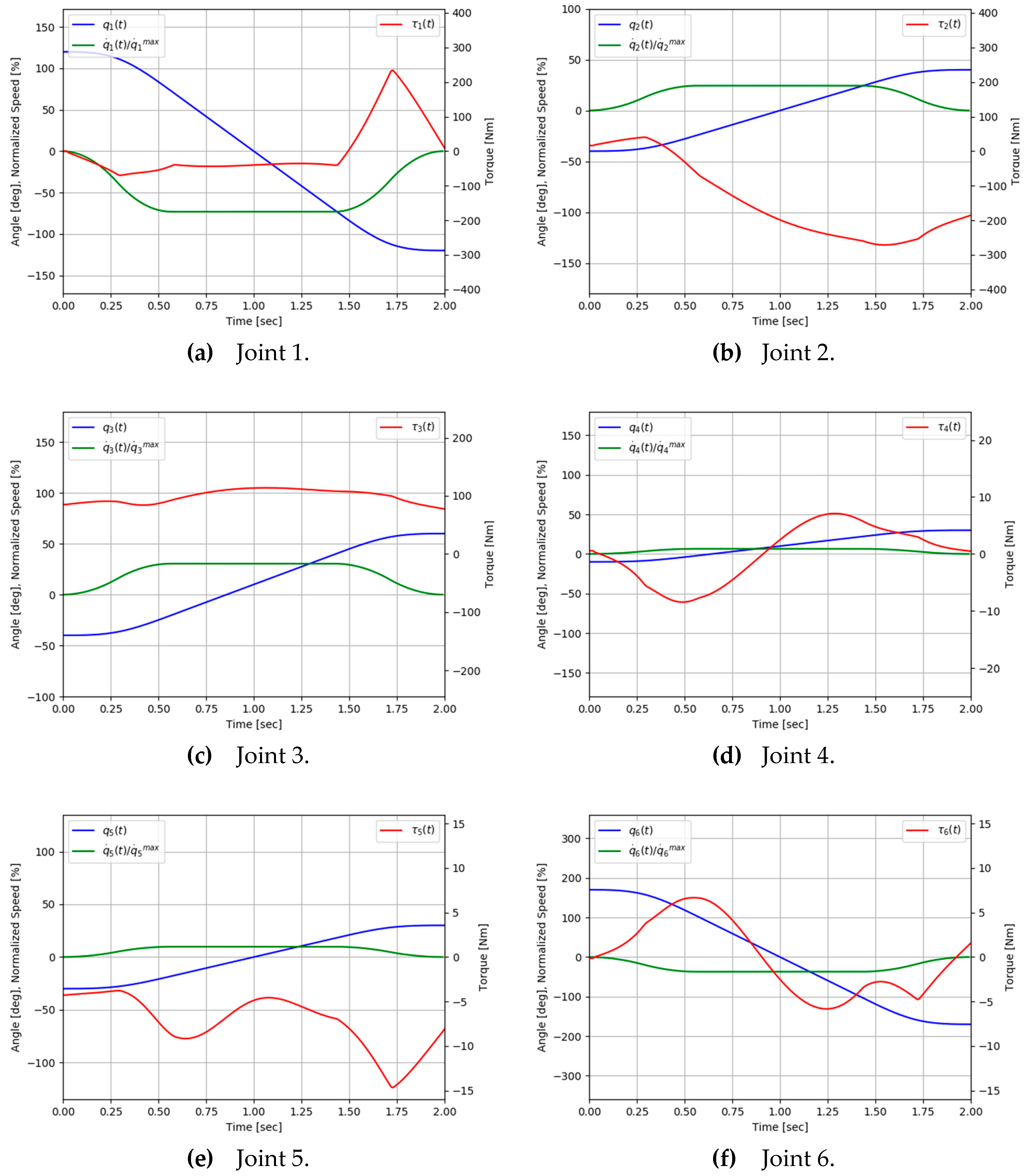
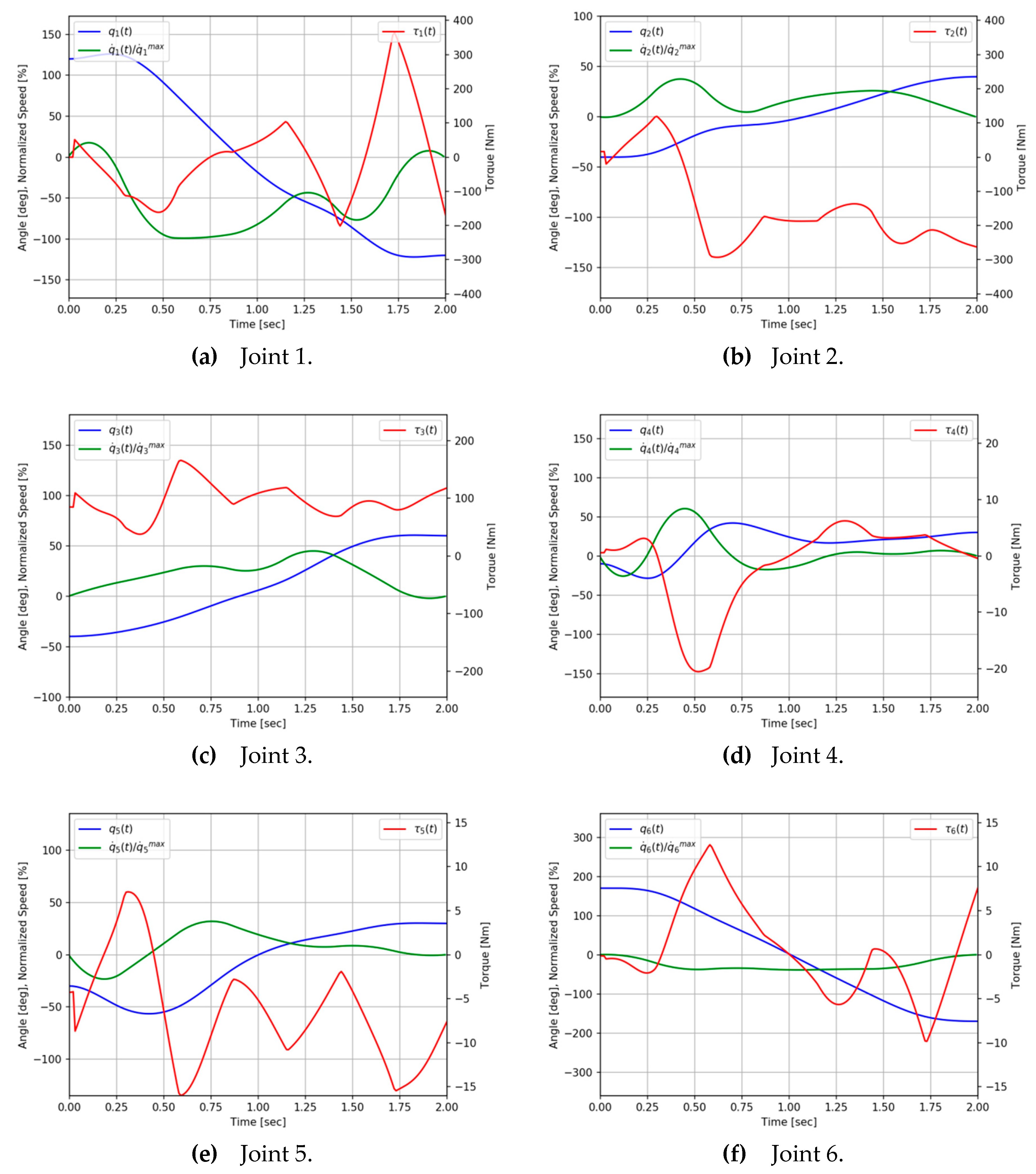
Figure 5 and Figure 6 represent the initial and the optimal motion profiles, respectively, for the case of $t_f=2$ s. Each joint begins to move at the initial angle and stops at the final angle, which are given in Table 4, at the end of the cycle time $t_f$. In the initial motion, the speed is uniform except for the initial and final acceleration/deceleration of the cycle time, while in the optimal motion, the speed fluctuates significantly. In particular, for optimal motion, it can be seen that the speed of joint 1 and torque of joint 5 reach the lower limit in 0.6 s and remain within the bound in Table 3 for the rest of the time (Figure 6).

Since the spline order was set to 3, it was possible to obtain a continuous motion profile up to the second derivative of the displacement, and it was confirmed that the profile of the driving torque also has a continuous waveform.

6. Conclusions

In this study, a numerical method to design robot motions for system-level life test of drive components of robot is developed. The major results of the paper are summarized as follows.

In order to derive the robot motion that makes the acceleration factor of each joint equal, we formulated a robot motion optimization problem that minimizes the AM-GM ratio of the acceleration factor of each joint.

Starting from the initially linear motion, a global optimal robot motion was derived that make the objective function of the optimization problem converges to zero. The optimal robot motion was shown to be $C_2$ continuous and make the acceleration factor of each joint equal.

Using the parameters of an actual 6-DoF industrial robot, global optimal robot motions were obtained for various cycle times and it was confirmed that the acceleration factor is inversely proportional to the cycle time.

It is expected that the motion optimization method proposed in the present study can be utilized to design a test mode for performing a system-level accelerated life test in which the robot drive component composed of a servo motor and a gearbox are mounted on the robot.

The results obtained so far assume the cycle time and initial and final posture of the robot are the fixed data of the optimization problem and consider only the trajectory of joint variables as the optimization variables.

In future work, we will explore more efficient test modes by including the robot’s cycle time, initial and final posture of robot, inertial parameter of the weight in the optimization variables. The effect of spline order and initial robot motion on the optimal solution will also be explored further in future studies.