Abstract
High-accuracy and dependable prediction of the bias of space-borne atomic clocks is extremely crucial for the normal operation of the satellites in the case of interrupted communication. Currently, the clock bias prediction for the Chinese BeiDou Navigation Satellite System (BDS) remains still a huge challenge. To develop a high-precision approach for forecasting satellite clock bias (SCB) in allusion to analyze the shortcomings of the exponential smoothing (ES) model, a modified ES model is proposed hereof, especially for BDS-2 satellites. Firstly, the basic ES models and their prediction mechanism are introduced. As the smoothing coefficient is difficult to determine, this leads to increasing fitting errors and poor forecast results. This issue is addressed by introducing a dynamic “thick near thin far (TNTF)” principle based on the sliding windows (SW) to optimize the best smoothing coefficient. Furthermore, to enhance the short-term forecasted accuracy of the ES model, the gray model (GM) is adopted to learn the fitting residuals of the ES model and combine the forecasted results of the ES model with the predicted results of the GM model from error learning (ES + GM). Compared with the single ES models, the experimental results show that the short-term forecast based on the ES + GM models is improved remarkably, especially for the combination of the three ES model and GM model (ES3 + GM). To further improve the medium-term prediction accuracy of the ES model, the new algorithms in ES with GM error learning based on the SW (ES + GM + SW) are presented. Through examples analysis, compared with the single ES2 (ES3) model, results indicate that (1) the average forecast precision of the new algorithms ES2 + GM + SW (ES3 + GM + SW) can be dramatically enhanced by 49.10% (56.40%) from 5.56 ns (6.77 ns) to 2.83 ns (2.95 ns); (2) the average forecast stability of the new algorithms ES2 + GM + SW (ES3 + GM + SW) is also observably boosted by 53.40% (49.60%) from 8.99 ns (16.13 ns) to 4.19 ns (8.13 ns). These new coupling forecast models proposed in this contribution are more effective in clock bias prediction both forecast accuracy and forecast stability.
1. Introduction
The Chinese Beidou Navigation Satellite System (BDS), to date, has completed the construction of its regional system BDS-2, which consists of 15 satellites [1]. The system can provide positioning, navigation, timing, and short message communication services for users in the Asia and Pacific. Over the past few years, it has made great strides in building global navigation systems such as BDS-3. By the end of 2018, a total of 19 BDS-3 satellites had been launched to enable the primary system for global services. With a total of 33 operational satellites, namely, 5 geostationary earth orbits (GEO), 7 inclined geosynchronous orbits (IGSO), and 21 medium earth orbits (MEO), the standard positioning accuracy of the orbits is achieved 5 m in both horizontal and vertical directions for the Asia-Pacific users and 10 m for global users approximately. By 23 June 2020, with the successful launch of the 55th networking satellite, it marks the complete networking of the BDS [2].
As one of the vital payloads of the Global Navigation Satellite System (GNSS), the performance of the satellite clocks and the accuracy, stability, and reliability of satellite clock bias (SCB) prediction are one of the critical factors affecting the positioning, navigation, and timing (PNT) service capabilities of the whole system [3,4,5]. Due to the rapid development of navigation satellite technology and its widespread use in practical applications, users’ requirements for accuracy are getting higher and higher. Many factors affect the capability of the PNT services, among which the impact of the SCBs is one of the most important factors [6,7]. Even a clock bias of 1 ns will produce a range error of 0.3 m approximately, which seriously influences the positioning and timing accuracy of navigation systems [8,9]. In order to meet the requirements of users for centimeter-level positioning, it is essential to establish a high-precision time system. The clock bias products released by the international IGS server are a post-precision clock bias file with high accuracy, but the acquisition time is longer and cannot fulfill the necessities of real-time positioning [10,11,12]. The improvement of the precision of clock bias forecast will contribute to the acquisition of a priori information required for satellite autonomous navigation and the ability to improve precise point positioning (PPP) accuracy [13,14,15]. Therefore, studying how to further the stability and accuracy of clock bias prediction is of paramount importance for boosting the quality of clock bias products and the ability of navigation and positioning.
At present, in order to enhance the precision level of SCBs prediction, many scholars had conducted multi-angle, multi-directional, and in-depth studies on SCBs prediction from various aspects, and a variety of clock bias prediction models had been established, e.g., polynomial prediction model, gray model (GM), auto-regressive moving average model (ARMA), spectrum analysis model (SAM), Least Squares Support Vector Machines (LSSVM), functional network, etc. [16,17,18,19,20,21]. Since the interruption of satellite clock information will affect the accuracy of real-time PPP, some methods, such as the optimal arc length identifying, diverse polynomial power forecasting and empirical model made of a sixth-power harmonic function, etc., were proposed as a way to build up the performance of real-time PPP [22,23,24]. Furthermore, a predicted method of clock bias with a wavelet neural network (WNN) model was put forth, and some outcomes were obtained via the prediction tests. Compared with the IGU-P clock bias products, this method could better improve the prediction accuracy, but this approach did not consider the periodic errors and the frequency shift errors [25]. Then, considering the characteristics of the rate of change of the clock bias, an improved WNN model (its activation function was reconstructed) was put forward to predict SCBs of the GPS satellites, and the prediction results showed the model had higher prediction accuracy and robustness [26]. A mathematical approach based on stochastic differential equations was presented to forecast the behavior of in-orbit atomic clocks. Concurrently, they considered respective diverse situations with conclusive and stochastic signatures and optimized prediction results of clock bias. The most considerable issue was that the structure of this model was complex [27].
Nevertheless, the characteristics of the clock bias of the BDS are different from those of Galileo, GLONASS, and GPS because of its special constellation, which involves MEO satellites, GEO satellites, and IGSO satellites. Hence, the forecasting models of the Galileo, GLONASS, and GPS clock bias cannot be simply applied mechanically in the BDS-2 clock bias forecast. In 2020, the fractal behavior of the BDS clock bias was demonstrated by using the moving-average rescaled range analysis approach, and the results of this study suggested that the BDS clock bias had a memory [28]. Further, because of the advantages of simple modeling, easy calculation, less data to be stored, and the ability to quickly calculate new predicted values from recent observed values, the exponential smoothing (ES) model is widely concerned in time series forecasting, such as transportation, power load forecasting, industry, and finance [29,30,31,32]. Up to now, very few studies have focused on the ES model in satellite clock forecasting. The ES model was first introduced into the short-term, medium-term, and long-term prediction of clock bias in 2017, but the selection of the smoothing coefficient was blind [33]. The 0.618 method was used to search for the best smoothing coefficient, and then, the model was established to predict the power load by using the found optimal smoothing coefficient. However, the optimization method was complex in operation and the forecast result was poor [34]. In the ES model, the determination of the smoothing coefficient is very complicated. In order to address this challenge, the “thick near thin far (TNTF)” principle is introduced to search for the best smoothing coefficient for better prediction. Then, in order to weaken the cumulative effect of errors due to the increase in forecast time, the idea of a sliding window (SW) is used to boost the forecast performance of the ES model employing the approach of a dynamic smoothing coefficient (ES based on SW). Besides, to further improve the forecast performance of the ES model, the GM model is used to learn the fitting error sequence of the ES model in the modeling process, and an SW is also adopted in the process (ES + GM based on SW), and then, the prediction results of the ES model and the GM model are combined as the final prediction clock bias. All these coupling algorithms are demonstrated by examples.
The remaining paper is organized as follows. The prediction theory of the ES + GM based on the SW idea is introduced—which includes the prediction principle of the ES method, the process of searching for the best smoothing coefficients utilizing the TNTF principle, the prediction principle of the ES model based on the SW idea, and the prediction principle of the ES + GM based on the SW idea—in Section 2. The sources of experimental data and the evaluation criteria used to evaluate the prediction performance of these coupling algorithms are introduced in Section 3. In Section 4, the forecasting performance of these coupling algorithms is demonstrated through examples and the forecasting advantages of these coupling algorithms are also analyzed in this section. Finally, some outcomes are drawn in Section 5.
2. Theory of Improved Exponential Smoothing Method Prediction
The modeling principles of the basic one exponential smoothing (ES1) model, two exponential smoothing (ES2) model, and three exponential smoothing (ES3) model are introduced first. Then, the principle and process of searching for the optimal smoothing coefficient using the TNTF principle is described in detail. Meanwhile, the prediction principles of the ES model based on the SW idea are introduced. Finally, the forecasting principles of the combined prediction method of the ES model and the GM model based on the SW idea are presented.
2.1. Exponential Smoothing Prediction Model
The ES model is a predicting method that is a weighted average of the clock bias time series observed in the past. The basic idea is that each time series has its inherent characteristics, that is, there is a certain basic mathematical model. However, the time series of actual observed clock bias not only embodies the above basic ideas but also reflects the characteristics of its random variation. In general, the impact of historical clock bias time series on future clock bias decreases with time gradually. Therefore, a more practical approach should be that the ES value of clock bias at the time is equal to the weighted average of the actual observed value of clock bias at the time and the ES value of clock bias at the time . In other words, the influence of the maximum and minimum is eliminated in the historical clock bias data to obtain the smoothed value of the clock bias time series. These smoothed clock biases are used as the forecast value of the clock bias at the future time.
In the whole forecasting process, the ES model can continuously correct new forecast values using forecast errors, i.e., the principle of “error feedback” can be utilized to correct the sequences of the forecasted clock bias, to boost the accuracy of the forecasted values of clock bias. The detailed process of the ES model is calculated as follows.
Suppose the current time is , and the observed value of the corresponding clock error series is , then the ES1 value of the clock bias time series at this time is [35,36]
where and refer to the ES1 value of the observed clock bias time series at the time and , respectively; denotes the smoothing coefficient; and is the time series of the observed clock bias at the time .
Equation (1) can be described as follows:
Combined Equations (1) and (2) can be obtained as follows:
At the time , the prediction model for the ES1 method can be written as
where indicates the predicted value of the observed clock bias time series at the time . It can be seen from Equation (4) that the predicted value of clock bias at time is the exponential smoothing value at time .
From Equations (1) and (4), the following equation can be derived.
The ES2 is performed based on ES1, and then, the value of ES2 at time is
where refer to the ES1 value of the observed clock bias sequences at time ; and represent the ES2 values of the observed clock bias sequences at the time and , respectively; and is the smoothing coefficient.
In the same way, the ES3 is performed based on ES2, then the value of ES3 at time is
where refers to the ES2 value of the observed clock bias sequences at time ; and represent the ES3 values of the observed clock bias sequences at the time and , respectively; and is the smoothing coefficient.
The prediction model for the ES2 method can be written as [37]
where ; represents the prediction value of the observed clock bias sequences at the time .
The prediction model for the ES3 method can be written as [37]
where,
and represents the forecast value of the observed clock bias sequences at the time .
Since the ES method is a recursive calculation formula, for the convenience of calculation, it is usually expressed as follows:
The most critical problem of the ES prediction model is how to determine an appropriate smoothing coefficient accurately. Since different will have a larger influence on the forecast result, the value of should be chosen between the interval according to the specific situation of the clock bias sequences. The value of reflects the degree of correction. The larger the value of , the larger the degree of correction; the smaller the value of , the smaller the degree of correction. Generally, when there is a big random fluctuation in the time series data of the clock bias, a big should be selected to keep up with the recent changes in the clock bias quickly. When the time series of the clock bias is relatively stable, a smaller should be selected. To address this conundrum that the smoothing coefficient is hard to determine in the ES forecast model, the principle of the TNTF is adopted to optimize the smoothing coefficient to achieve a better forecasting results in this contribution.
The ES1 prediction model is applicable to time series with less pronounced change trends. The ES2 prediction model is suitable for time series like linear variation trends. The ES3 prediction model is mainly applied to time series with quasi-nonlinear variation trends. Considering the characteristics of clock bias time series changes, we analyze the forecasting performance of the ES2 model, the ES3 model, and the forecasting models using different modeling strategies for SCBs.
2.2. Optimize the Smoothing Coefficient Using the “TNTF” Principle
The TNTF principle means that the trend of clock bias over the future period depends more on the recent development law in the historical clock bias, while the correlation of the development trend between long-term historical and the future clock bias is weak. Principle TNTF has a variety of specific implementation methods, the method adopted in this contribution is to introduce a fitting error weight coefficient (varies from 0 to 1), and the fitting error weight coefficient is divided into 9 equal parts (0.1, 0.2,…,0.9). The fitting errors of the model are determined by employing the weighted mean absolute percentage error (WMAPE) as follows [38].
where the value of represents the degree of TNTF principle; is the analog value of the clock bias; is the observed value of the clock bias; is the number of the clock bias participating in modeling.
The most commonly used methods to search for the optimal smoothing coefficient include the theoretical method and the empirical approach. In this contribution, the equipartition method is adopted. Compared with other methods, the equipartition method has the advantages of simplicity and intuition. The search process of is as follows.
(1) Values assigned to , respectively.
(2) Divide () into 999 parts evenly, namely ().
(3) We substitute into Equations (3), (6), and (7) in turn, and then the corresponding , , and can be calculated by combining Equation (10).
(4) The analog values of the ES method can be obtained by substituting the calculated , , and into Equations (8) and (9), respectively.
(5) By substituting the analog values of the calculated clock bias and the actual observed values of the clock bias and the given into Equation (11), the values WMAPE corresponding to a set of can be obtained.
(6) Repeat operation steps from (2) to (5) for each given to obtain 9 × 999 corresponding WMAPE, and then, compare these values. The corresponding to the smallest WMAPE is the optimal smoothing coefficient searched out. The flow of the specific optimization process is depicted in Figure 1.
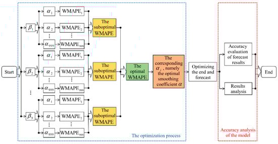
Figure 1.
Flow chart of the optimization process of the thick near thin far (TNTF) principle.
2.3. Prediction Principle of ES Based on Sliding Window
Since the smoothing coefficients of the ES method are difficult to determine and the error accumulation is relatively large as the forecast time increases, the algorithm is improved using the idea of sliding windows (SW) in forecasting SCBs. The flow of the SW method for forecasting SCBs is shown in Figure 2. The flow of the improved algorithm using the SW is shown in Figure 3. The process of forecasting the clock bias is divided into steps. In each step, the best smoothing coefficient is chosen to reduce the prediction errors. The range of the smoothing coefficient is (0,1). In the first step, to obtain the optimal smoothing coefficient, the interval of (0,1) is divided into 999 parts on average, and the first value is 0.001 and the last value is 0.999. The above TNTF principle is employed in searching for the best smoothing coefficient. The found best smoothing coefficient is then used to develop an ES model to forecast the clock bias with the following length of L1. In the second step, the clock bias forecasted in the first step is used as the fitting sample for the ES model, and then, the best smoothing coefficient can be found employing the same method as in the first step. Based on the found optimal smoothing coefficient, an ES model is established to forecast the clock bias of the following length of L2. Repeat this until the end of the nth step. The final forecast clock bias is the sum of the forecast clock bias for each step. Taken together, the detailed steps for the ES model using the SW (ES + SW) are as follows. The flow of the ES + SW models are depicted in Figure 4.
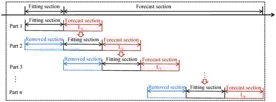
Figure 2.
Prediction flow chart of the sliding window method.
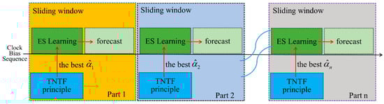
Figure 3.
Flow chart of exponential smoothing (ES) clock bias prediction using a sliding window.
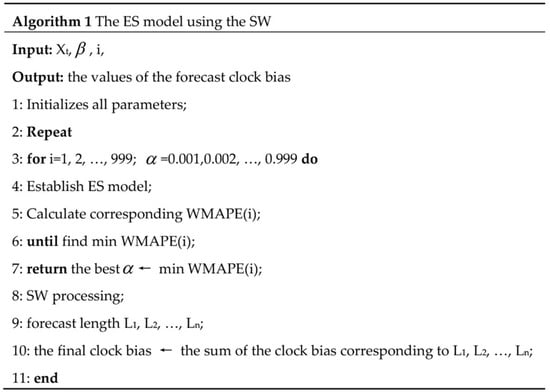
Figure 4.
Flow of the ES model using a sliding window.
Take the first part as an example, and the rest of the parts are similar to the first one.
Step 1 (parameter initialization). All parameters of the algorithm are initialized.
Step 2 (searching for the best smoothing coefficient). The interval of (0,1) is divided into 999 parts equally, and the first value is 0.001, and the last value is 0.999. The TNTF principle is adopted to search for the best smoothing coefficient.
Step 3 (modeling and forecasting). An ES model is developed for forecasting based on the searched best smoothing coefficients.
Step 4 (SW processing). Take the previous steps as an example; in the first step, the forecast is stopped when the length of the forecast reaches L1. In the second step, the clock bias from the first step forecast is used as the fitting sample for modeling, and the forecast is stopped when the length of the forecast reaches L2. Repeat until the end of the nth step, and the final complete forecast clock bias sequences are the sum of the clock errors corresponding to L1 + L2 + …+Ln.
2.4. Prediction Principle of ES + GM Using Sliding Window
To further boost the accuracy of clock bias prediction, the GM model is used to learn the fitting errors generated by the ES model during the modeling process, and forecast the value of the fitting errors of the ES model. The final prediction values of clock bias can be obtained by combining the predicted values of the ES model and the GM model. The detailed process of this fusion algorithm is shown in Figure 5. The specific steps for this fusion algorithm of the ES model and the GM model using the SW (ES + GM + SW) are as follows.
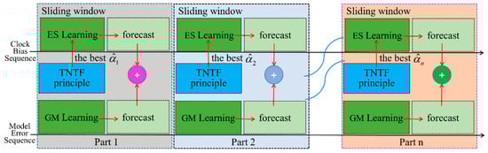
Figure 5.
Flow chart of ES + GM clock bias prediction using a sliding window. GM, gray model.
Take the first part as an example, and the rest of the parts are similar to it. Steps 1 to 3 of ES + GM + SW are the same as ES + SW (see Section 2.3).
Step 4 (GM forecast). During step 3, an ES model is built based on the optimal smoothing coefficients, which generates a fitting error series during the modeling process, and then, the GM model is used to learn the fitting error series and forecast.
Step 5 (SW processing). The processing method of this step is similar to step 4 of the ES model based on the SW.
Step 6 (fusion forecasting). Combining the prediction value of the ES model and the prediction value of the GM model in each part, the final prediction value of clock bias can be obtained.
In step 4, the GM model is used to learn the fitting error sequence of the ES model, and the modeling process is as follows.
Suppose that the fitting error sequence of the ES model is , a new sequence is generated by one-time accumulation as follows [39].
Establish a first-power differential equation for the sequences as shown below.
The first-power differential equation (13) could be described by the matrix equation form (14) after discretization.
where,
The least-squares solution to the matrix Equation (14) is obtained employing the least-squares method (LSM) as follows.
Substituting Equation (16) into Equation (13), the following Equation (17) can be obtained.
The solution of the time response function (17) can be expressed as
Since sequence is the cumulative sequence of sequence , the prediction model for the fitting error sequence of the ES model can be written as follows:
3. Experimental Data and Evaluation Indicators
The data source selected for the experiment and analysis is first introduced in detail. Furthermore, evaluation indicators used to evaluate the prediction performance of these models are then presented.
3.1. Experimental Datasets
To fully investigate the forecasting performance of these model aforementioned in this contribution, the clock bias of the BDS-2 satellites with the first day to the second day of the 737 weeks (16–17 February 2020) released by the International GNSS Monitoring and Assessment System (iGMAS) were selected as experimental data.
In order to make the research results provide some references for PPP, these data were interpolated into the clock bias of the 30 s intervals before modeling and predicting. There are three types of BDS-2 satellites: the GEO satellites, the IGSO satellites, and the MEO satellites, with a total of 15 satellites, containing 5 GEO satellites, 7 IGSO satellites, and 3 MEO satellites. The clock bias of two satellites with continuous and complete data with no clock jumps and outliers were selected from each type of satellite for the experiments. The selected satellites are C 01 (GEO), C 05 (GEO), C 10 (IGSO), C 16 (IGSO), C 11 (MEO), and C 12 (MEO), respectively, with a total of six satellites. As of February 2020, information about these satellites is listed in Table 1 [40].

Table 1.
Information on selected satellites (as of February 2020).
3.2. Evaluation Criteria
To fully assess the predicted performances of these models, the root mean square (RMS) and Range (the absolute value of the error between the maximum errors and the minimum errors) are used as the statistics to evaluate the models’ forecast results. Among them, the RMS represents the forecast accuracy of the model, and the Range denotes the stability of the model. The expression of RMS and Range can be written as [41]
where, refer to the forecast error of the model; and indicate the predicted and real clock bias in epoch , respectively; is the number of observed clock bias. and represent the maximum and minimum value of the model prediction errors, respectively.
As shown in Equations (20) and (21), values of RMS and Range will be obtained by using different models. Also, the smaller the values of RMS and Range represent the better-predicted performances of the model.
4. Results and Discussion
Five modeling strategies are used to predict SCBs for short-term prediction first, and the forecasting performance of these models is analyzed in detail. Then, the medium-term prediction of SCBs is performed using seven modeling strategies, and the prediction performance of these models is analyzed.
4.1. Short-Term Forecast Performance Analysis
The first day clock bias data of the 737 weeks (16 February 2020) are used to build a model. Then, the established model can be applied to forecast the clock bias data for the next 6 h. Since the length of the forecast is not long, SW processing is not adopted. The modeling strategies are as follows.
(1) The ES2 and ES3 models are built using the first day clock bias data of the 737 weeks (16 February 2020), respectively, and the established ES2 and ES3 models can be employed to predict the next 6 h clock bias data.
(2) To boost the forecast accuracy of the ES2 (ES3) model, the GM model is utilized to learn the fitting error of the ES2 (ES3) model during the modeling process. In other words, a combined forecasting model of the ES2 (ES3) model and the GM model (abbreviated as ES2 + GM and ES3 + GM) is developed. The coupling model algorithm is as follows. First, an ES2 (ES3) model is set up employing the clock bias data of the first day of the 737 weeks (16 February 2020), and the established ES2 (ES3) model can be applied to predict the next 6 h clock bias data. Then, the GM model is applied to learn the fitting error of the ES2 (ES3) model during the modeling process, and the predicted results of the fitting error for the next 6 h will be obtained. The final predicted clock bias is the sum of the clock bias predicted by the ES2 (ES3) model and the predicted value of the fitting error predicted by the GM model.
(3) Besides this, to serve as a comparison algorithm, the single GM model is built using the clock error of the first day of the 737 weeks (16 February 2020) and forecast the clock bias data of the next 6 h.
For convenience, the labels “GM,” “ES2,” “ES2 + GM,” “ES2 + SW,” “ES2 + GM + SW,” “ES3,” “ES3 + GM,” “ES3 + SW,” and “ES3 + GM + SW,” stand for the gray model, two exponential smoothing model, the combined model using the gray model to learn the fitting error of two exponential smoothing model, two exponential smoothing model using sliding windows, the combination of two exponential smoothing model and gray model using sliding windows, three exponential smoothing model, the combined model using the gray model to learn the fitting error of three exponential smoothing model, three exponential smoothing model using sliding windows, and the combination of three exponential smoothing model and gray model using sliding windows, respectively, in named system of Figure 6, Figure 7, Figure 8, Figure 9, Figure 10, Figure 11, Figure 12 and Figure 13 and Table 2, Table 3, Table 4 and Table 5.
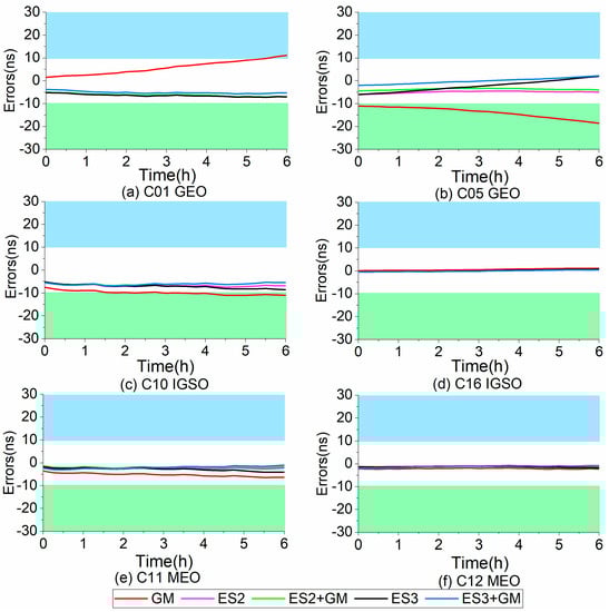
Figure 6.
Variation diagram of 6 h satellite clock bias forecast errors using different models: (a) is the changes of the C 01 SCBs forecast, (b) is the changes of the C 05 SCBs forecast, (c) is the changes of the C 10 SCBs forecast; (d) is the changes of the C 16 SCBs forecast, (e) is the changes of the C 11 SCBs forecast, and (f) is the changes of the C 12 SCBs forecast.
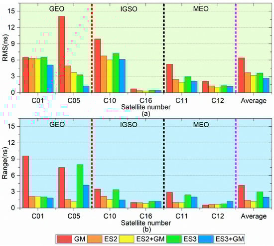
Figure 7.
Variation diagram of 6 h forecast accuracy (RMS) and stability (Range) using different models: (a) is the changes of RMS, and (b) is the changes of Range.
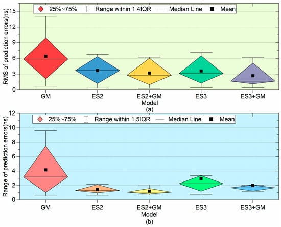
Figure 8.
Boxplot change diagram of 6 h prediction accuracy (a) and stability (b) using different models.
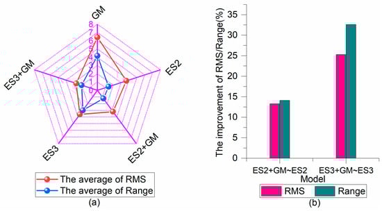
Figure 9.
The average accuracy (RMS), stability (Range), and improvement percentage of 6 h forecast using different models: (a) is the changes of RMS and Range, and (b) is the changes of improvement percentage of RMS and Range.
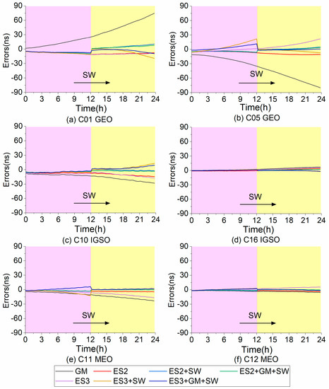
Figure 10.
Variation diagram of 24 h satellite clock bias forecast errors using different models: (a) is the changes of the C 01 SCBs forecast, (b) is the changes of the C 05 SCBs forecast, (c) is the changes of the C 10 SCBs forecast; (d) is the changes of the C 16 SCBs forecast, (e) is the changes of the C 11 SCBs forecast, and (f) is the changes of the C 12 SCBs forecast.
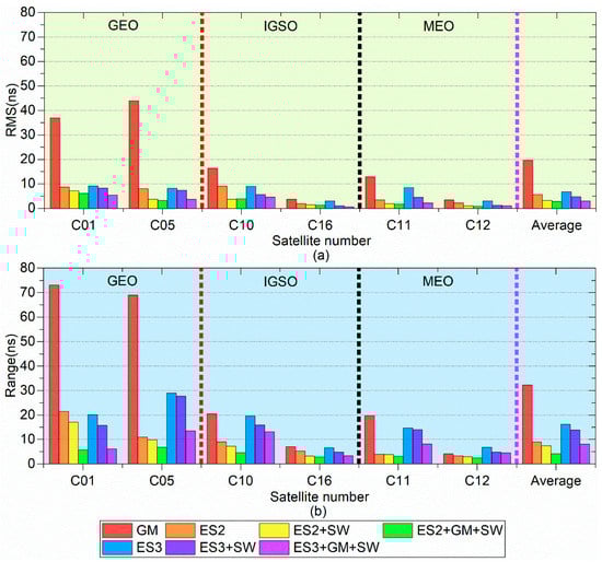
Figure 11.
Variation diagram of 24 h forecast accuracy (RMS) and stability (Range) using different models: (a) is the changes of RMS, and (b) is the changes of Range.
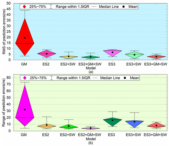
Figure 12.
Boxplot change diagram of 24 h prediction accuracy (a) and stability (b) using different models.
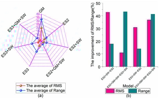
Figure 13.
Change of average accuracy (RMS), stability (Range), and improvement rate of 24 h forecast using different models: (a) is the changes of RMS and Range, and (b) is the changes of improvement percentage of RMS and Range.
Table 2.
Statistics of the different models for 6 h prediction (ns).
Table 3.
Statistics of the average prediction precision (RMS), stability (Range), and improvement of the different models for 6 h (ns).
Table 4.
Statistics of the different models for 24 prediction (ns).
Table 5.
Statistics of the average prediction precision (RMS), stability (Range), and improvement of the different models for 24 h (ns).
Figure 6 shows the error change of 6 h SCBs forecast using different models, where Figure 6a is the changes of the C 01 (GEO) SCBs forecast, Figure 6b is the changes of the C 05 (GEO) SCBs forecast, Figure 6c is the changes of the C 10 (IGSO) SCBs forecast, Figure 6d is the changes of the C 16 (IGSO) SCBs forecast, Figure 6e is the changes of the C 11 (MEO) SCBs forecast, and Figure 6f is the changes of the C 12 (MEO) SCBs forecast.
Figure 7 shows the variation of 6 h forecast accuracy (RMS) and stability (Range) using different models, where Figure 7a is the changes of forecast accuracy (RMS) and average forecast accuracy (RMS), and Figure 7b is the changes of forecast stability (Range) and average forecast stability (Range).
Figure 8 shows the boxplot changes of 6 h prediction accuracy (RMS) and stability (Range) using different models, where Figure 8a is the boxplot changes of RMS of prediction errors, and Figure 8b is the boxplot changes of Range of prediction errors.
Figure 9 shows the changes of the average accuracy (RMS), stability (Range), and improvement percentage for 6 h prediction using different models, where Figure 9a is the changes of the average of RMS and Range, Figure 9b is the improvement of the ES2 + GM (ES3 + GM) model compared to the ES2 (ES3) model The 6 h prediction statistics for the different satellites with different models are listed in Table 2, and the statistics of the average forecast precision (RMS), stability (Range), and improvement of the different models for 6 h prediction are shown in Table 3.
From Figure 6, Figure 7, Figure 8 and Figure 9 and Table 2 and Table 3, we can see that in terms of a single model, the average forecast accuracy of the ES3 model is roughly the same as that of the ES2 model, while the average forecast accuracy of the ES3 model is slightly better than that of the ES2 model. The average forecast accuracy of the GM model is worse than that of the ES2 model. As for the combined model, the GM model is used to learn the fitting errors of the ES model and forecast the values of the fitting errors. The comparative analysis between the combined models (ES2 + GM and ES3 + GM) and the single ES models (ES2 and ES3) show that the prediction results of the combined ES model can boost the forecast performance of the ES model. Especially, the performance enhancement of the ES3 model is remarkable and their prediction accuracy has been further heightened. Compared with the single ES (ES2 and ES3) model, the average forecast accuracy of the ES2 + GM (ES3 + GM) model has been increased by 13.30% (25.30%) from 3.68 ns (3.59 ns) to 3.19 ns (2.68 ns), and the average forecast stability of the ES2 + GM (ES3 + GM) model has been increased by 14.10% (32.60%) from 1.42 ns (2.98 ns) to 1.22 ns (2.01 ns).
In general, apart from the prediction algorithm, the MEO satellites accomplish a fairly superior forecast accuracy, followed by IGSO satellites. The worst is GEO satellites, which are probably related to the poor observed structures and observations.
4.2. Medium-Term Forecast Performance Analysis
The clock bias data of the first day of the 737 weeks (16 February 2020) are employed to build a model. Then, the established model can be applied to predict the next 24 h clock bias. The modeling strategies are as follows.
(1) The ES2 and ES3 models are established employing the clock bias data of the first day of the 737 weeks (16 February 2020), respectively, and the established ES2 and ES3 models can be employed to predict the next 24 h clock bias data.
(2) Because of the longer forecast length, to boost the forecast accuracy of the ES2 (ES3) model, SW processing is adopted, that is, a combined forecasting model of the ES2 (ES3) model using the SW processing (abbreviated as ES2 + SW and ES3 + SW), is established. The coupling model algorithm is as follows. The length of the forecast is divided into two parts equally. First, an ES2 (ES3) model is developed by using the clock bias of the first day of 737 weeks (16 February 2020) to forecast the next 12 h clock bias data. Then, the 12 h clock bias predicted in the previous step and the last 12 h clock bias the first day of the 737 weeks (16 February 2020), the of 24 h clock bias data are used to establish an ES2 (ES3) model to forecast the clock bias for the next 12 h. Finally, the final forecasted clock bias is the combination of the clock bias of the first part of the forecast and the clock bias of the second part of the forecast.
(3) Since the forecast time is relatively long, to further improve the forecast accuracy of the ES2 (ES3) model, the GM model is applied to learn the fitting error of the ES2 (ES3) model during the modeling process, and then, the SW processing method is employed to establish a combination forecast model: the ES2 (ES3) model and GM model using SW processing (abbreviated as ES2 + GM + SW and ES3 + GM + SW). The coupling model algorithm is as follows. The length of the forecast is divided into two parts equally. First, an ES2 (ES3) model is developed by using the clock bias of the first day of 737 weeks (16 February 2020) to predict the next 12 h clock bias data. Then, the GM model is applied to learn the fitting error of the ES2 (ES3) model during the modeling process, and the predicted values of the fitting error for the next 12 h will be obtained. The clock bias of the first part is equal to the sum of the clock bias predicted by the ES2 (ES3) model and the forecast value of the fitting error predicted by the GM model. Then, the SW processing is adopted, and the 12 h clock bias predicted in the previous step and the last 12 h clock bias of the first day of the 737 weeks (16 February 2020), the 24 h clock bias data, are used to establish an ES2 (ES3) model to forecast the clock bias for the next 12 h. Then, using the same processing method as the first part, the clock bias of the second part is equal to the sum of the clock bias predicted by the ES2 (ES3) model and the forecast value of the fitting error predicted by the GM model. Finally, the final forecasted clock bias is the combination of the clock bias of the first part and the clock bias of the second part.
(4) Besides this, the single GM model as a comparison algorithm is established, employing the clock bias of the first day of the 737 weeks (16 February 2020) and forecast the clock bias data of the next 24 h.
Figure 10 shows the error changes of 24 h SCBs forecast using different prediction models, where Figure 10a is the changes of the C 01 (GEO) SCBs forecast, Figure 10b is the changes of the C 05 (GEO) SCBs forecast, Figure 10c is the changes of the C 10 (IGSO) SCBs forecast, Figure 10d is the changes of the C 16 (IGSO) SCBs forecast, Figure 10e is the changes of the C 11 (MEO) SCBs forecast, and Figure 10f is the changes of the C 12 (MEO) SCBs forecast.
The changes in the bar chart for 24 h forecast accuracy (RMS) and stability (Range) using different models are shown in Figure 11, where Figure 11a is the changes of the forecast accuracy (RMS) for the different satellites, and Figure 11b is the changes of the forecast stability (Range) for the different satellites.
Figure 12 shows the boxplot changes of 24 h prediction accuracy and stability using different models, where Figure 12a is the boxplot changes of RMS of prediction errors, and Figure 12b is the boxplot changes of Range of prediction errors.
Figure 13 reveals the changes of the average accuracy (RMS), stability (Range), and improvement percentage for 24 h prediction, where Figure 13a is the changes of the average of RMS and Range, Figure 13b is the improvement of the ES2 + SW, ES2 + GM + SW, ES3 + SW, and ES3 + GM + SW model compared to the ES2, ES2 + SW, ES3, and ES3 + SW model, respectively. The 24 h prediction statistics for the different satellites with different models are exhibited in Table 4, and the Statistics of the average forecast precision (RMS), stability (Range), and improvement of the different models for 24 h prediction are shown in Table 5.
From Figure 10, Figure 11, Figure 12 and Figure 13 and Table 4 and Table 5, it can be seen that the medium-term forecast performance of the ES2 model is slightly better than that of the ES3 model with respect to single-model forecasting. These mean that the ES3 model is more suitable for short term forecast, while the ES2 model is more suitable for medium-term forecast by comparison with the abovementioned parts. Compared with the prediction performances of the ES2 model and the ES3 model, the GM model has a slightly worse performance in medium-term prediction. The forecast performance of both the ES2 model and ES3 model has been boosted to a great degree after using the SW processing.
Compared with the single ES2 (ES3) model, the average forecast accuracy of the combined model of the ES2 (ES3) model and the SW processing has been increased by 42.80% (31.00%) from 5.56 ns (6.77 ns) to 3.18 ns (4.67 ns), and the average forecast stability has been increased by 17.90% (14.10%) from 8.99 ns (16.13 ns) to 7.38 ns (13.86 ns). The aforementioned comparative analysis shows that the use of the SW processing strategy can significantly boost the forecast performance of the ES model, especially for the ES2 model, both in terms of forecast accuracy and forecast stability.
The forecast accuracy and stability of these fusion prediction algorithms are further improved by using the GM model to learn the fitting errors of the ES model in the modeling process followed based upon the SW processing. Compared with the single ES2 (ES3) model that does not use the GM model to learn the fitting error, the average forecast accuracy of these fusion algorithms is increased by 11.00% (36.80%) from 3.18 ns (4.67 ns) to 2.83 ns (2.95 ns), and the average forecast stability is increased by 43.20% (41.30%) from 7.38 ns (13.86 ns) to 4.19 ns (8.13 ns). Overall, the GM model is used to learn the fitting error of the ES model, and then the fusion prediction algorithm with the SW processing can significantly improve the performance of the ES model. In particular, the performance of the medium-term prediction of the ES3 model has been improved greatly. In addition, both single algorithm and fusion algorithm have better prediction performance for recently launched satellites than for early launched satellites.
5. Conclusions
In the applications of the GNSS, the clock bias forecast is a critical issue. The accuracy and stability of SCBs prediction determine the accuracy of satellite navigation and positioning directly. For purpose of improving the accuracy and stability of clock bias prediction, a new fusion prediction algorithm is proposed in this contribution to perform short-term and medium-term prediction of clock bias. The clock bias data of the BDS-2 satellites with the first day to the second day of the 737 weeks of the DOY released by the iGMAS are selected as experimental data to assess the prediction performance of these new models. For the comparison and analysis, the single GM, ES2, and ES3 models are regarded as reference, then the prediction performance of the ES2 + SW, ES3 + SW, ES2 + GM + SW, and ES3 + GM + SW model for clock bias are then analyzed.
As for the short-term clock bias prediction, the method of predicting after learning the fitting error for the ES model during the modeling process using the GM model can enhance the forecast performance of the ES model dramatically: both the forecast accuracy and the stability of the forecast. In particular, the average forecast accuracy of the ES3 model has the greatest improvement, up to 25.30% going from 3.59 ns to 2.68 ns, and the average forecast stability of the ES3 model has the greatest improvement, up to 32.60% going from 2.98 ns to 2.01 ns. With respect to the medium-term prediction of clock bias, the fusion prediction algorithm using two processing strategies can improve the forecasting performance of the ES model, whether in terms of forecast accuracy or forecast stability. Above all, the most significant improvement in the prediction performance of the ES model is achieved by using a GM model to learn the fitting errors during the modeling process, followed by an SW processing strategy. Its average forecast accuracy is improved by 49.10% (56.40%) from 5.56 ns (6.77 ns) to 2.83 ns (2.95 ns), and the average forecast stability is improved by 53.40% (49.60%) from 8.99 ns (16.13 ns) to 4.19 ns (8.13 ns), compared with the single ES2 (ES3) model.
Overall, this new fusion prediction algorithm is advantageous and can be used to forecast the BDS-2 clock bias with high-precision both in the short-term and medium-term. Therefore, it is recommended that this new algorithm can be utilized to predict clock bias for BDS-2 satellites. Furthermore, this study provides a theoretical reference for SCBs in terms of high-precision prediction and practical applications, and also provides a new guideline for continued research in SCBs forecast technology in the future.
Author Contributions
Y.Y. and M.H. designed the experiments. Y.Y. contributed to the tests and analyzed the data. T.D., C.W., and R.H. validated the experimental results and reviewed the paper. Y.Y. wrote the paper. All authors have read and agreed to the published version of the manuscript.
Funding
Funding supports from the Postdoctoral Science Foundation of China (No. 2019M650801) and Director′s Foundation of Institute of Microelectronics, Chinese Academy of Sciences (No. E0518101).
Acknowledgments
We thank the editors and the anonymous reviewers for their valuable comments and suggestions to improve the paper. Many thanks go to the IGS MGEX for providing clock bias products.
Conflicts of Interest
The authors declare no conflict of interest.
Abbreviations
| Abbreviation | The full name |
| BDS | BeiDou Navigation Satellite System |
| SCB | Satellite Clock Bias |
| ES | Exponential Smoothing |
| TNTF | Thick Near Thin Far |
| SW | Sliding Windows |
| GM | Gray Model |
| ES1 | One Exponential Smoothing |
| ES2 | Two Exponential Smoothing |
| ES3 | Three Exponential Smoothing |
| ES + SW | Exponential Smoothing using Sliding Windows |
| ES + GM | the combination model of the ES model and the GM |
| ES2 + GM | the combination model of the ES2 model and the GM |
| ES3 + GM | the combination model of the ES3 model and the GM |
| ES2 + GM + SW | the combination of the ES2 model and the GM using sliding windows |
| ES3 + GM + SW | the combination of the ES3 model and the GM using sliding windows |
| GNSS | Global Navigation Satellite System |
| GPS | Global Positioning System |
| GLONASS | GLObal NAvigation Satellite System |
| PNT | Positioning, navigation, and timing |
| IGS | International GNSS Service |
| PPP | Precise point positioning |
| ARMA | Auto-Regressive Moving Average model |
| SAM | Spectrum Analysis Model |
| LSSVM | Least Squares Support Vector Machines |
| WNN | Wavelet Neural Network |
| MEO | Medium Earth Orbit |
| GEO | Geosynchronous Earth Orbit |
| IGSO | Inclined Geosynchronous Satellite Orbit |
| WMAPE | Weighted Mean Absolute Percentage Error |
| iGMAS | international GNSS Monitoring & Assessment System |
| PRN | Pseudo-Random Noise code |
| LSM | Least Squares Method |
| RMS | Root Mean Square |
References
- CSNO. Development of the BeiDou Navigation Satellite System (Version 4.0). Available online: http://www.beidou.gov.cn/xt/gfxz/201912/P020191227337020425733.pdf (accessed on 15 October 2020).
- Tu, R.; Zhang, R.; Fan, L.H.; Han, J.Q.; Zhang, P.F.; Lu, X.C. Real-Time Detection of Orbital Maneuvers Using Epoch-Differenced Carrier Phase Observations and Broadcast Ephemeris Data: A Case Study of the BDS Dataset. Sensors 2020, 20, 4584. [Google Scholar] [CrossRef]
- Montenbruck, O.; Steigenberger, P.; Prange, L. The multi GNSS experiment (MGEX) of the international GNSS service (IGS)–achievements, prospects and challenges. Adv. Space Res. 2017, 59, 1671–1697. [Google Scholar] [CrossRef]
- Cai, C.; Gao, Y. GLONASS-based precise point positioning and performance analysis. Adv. Space Res. 2013, 51, 514–524. [Google Scholar] [CrossRef]
- Zhang, L.; Yang, H.; Gao, Y.; Yao, Y.; Xu, C. Evaluation and analysis of real-time precise orbits and clocks products from different IGS analysis centers. Adv. Space Res. 2018, 61, 2942–2954. [Google Scholar] [CrossRef]
- Ge, M.R.; Chen, J.P.; Dousa, J.; Gendt, G.; Wickert, J. A computationally efficient approach for estimating high-rate satellite clock corrections in realtime. GPS Solut. 2012, 16, 9–17. [Google Scholar] [CrossRef]
- Huang, G.W.; Cui, B.B.; Zhang, Q.; Fu, W.J.; Li, P.L. An Improved Predicted Model for BDS Ultra-Rapid Satellite Clock Offsets. Remote Sens. 2018, 10, 60. [Google Scholar] [CrossRef]
- Xu, B.; Wang, L.; Fu, W.; Chen, R.; Li, T.; Zhang, X. A Practical Adaptive Clock Offset Prediction Model for the Beidou-2 System. Remote Sens. 2019, 11, 1850. [Google Scholar] [CrossRef]
- He, L.; Zhou, H.; Wen, Y.; He, X. Improving Short Term Clock Prediction for BDS-2 Real-Time Precise Point Positioning. Sensors 2019, 12, 2762. [Google Scholar] [CrossRef]
- Senior, K.L.; Ray, J.R.; Beard, R.L. Characterization of periodic variations in the GPS satellite clocks. GPS Solut. 2008, 12, 211–225. [Google Scholar] [CrossRef]
- Heo, Y.J.; Cho, J. Improving prediction accuracy of GPS satellite clocks with periodic variation behavior. Meas. Sci. Technol. 2010, 21, 073001–073008. [Google Scholar] [CrossRef]
- Lu, J.C.; Zhang, C.; Zheng, Y.; Wang, R.P. Fusion-based Satellite Clock Bias Prediction Considering Characteristics and Fitted Residue. J. Navig. 2018, 71, 1–16. [Google Scholar] [CrossRef]
- Xu, A.; Xu, Z.; Xu, X. Precise Point Positioning Using the Regional BeiDou Navigation Satellite Constellation. J. Navig. 2014, 67, 523–537. [Google Scholar] [CrossRef]
- Zhao, Q.; Guo, J.; Hu, Z.; Shi, C.; Liu, J. Initial results of precise orbit and clock determination for compass navigation satellite system. J. Geod. 2013, 87, 475–486. [Google Scholar] [CrossRef]
- Hauschild, A.; Montenbruck, O.; Steigenberger, P. Short-term analysis of GNSS clocks. GPS Solut. 2013, 17, 295–307. [Google Scholar] [CrossRef]
- Wang, D.; Guo, R.; Xiao, S.; Xin, J.; Tang, T.; Yuan, Y. Atomic clock performance and combined clock error prediction for the new generation of BeiDou navigation satellites. Adv. Space Res. 2018, 63, 2889–2898. [Google Scholar] [CrossRef]
- Liang, Y.; Ren, C.; Yang, X.; Pang, G.; Lan, L. A grey model based on first differences in the application of satellite clock bias prediction. Chin. Astron. Astrophys. 2015, 40, 79–93. [Google Scholar] [CrossRef]
- Liu, Q.; Sun, J.; Chen, X.; Liu, J.; Zhang, Q. Application analysis of CPSO-LSSVM algorithm in AR clock error prediction. J. Jilin Univ. Eng. Technol. Ed. 2014, 44, 807–811. [Google Scholar]
- He, L.; Zhou, H.; Liu, Z.; Wen, Y.; He, X. Improving clock prediction algorithm for BDS-2/3 satellites based on LS-SVM method. Remote Sens. 2019, 11, 2554. [Google Scholar] [CrossRef]
- Wang, Y.; Lv, Z.; Ning, W.; Li, L.; Gong, X. Prediction of navigation satellite clock bias considering clock’s stochastic variation behavior with robust least square collocation. Acta Geod. Cartogr. Sin. 2016, 45, 646–655. [Google Scholar]
- Xu, B.; Wang, Y.; Yang, X. Navigation satellite clock error prediction based on functional network. Neural Process. Lett. 2013, 38, 305–320. [Google Scholar] [CrossRef]
- El-Mowafy, A.; Deo, M.; Kubo, N. Maintaining real-time precise point positioning during outages of orbit and clock corrections. GPS Solut. 2017, 21, 937–947. [Google Scholar] [CrossRef]
- Pan, L.; Zhang, X.; Li, X.; Liu, J.; Guo, F.; Yuan, Y. GPS inter-frequency clock bias modeling and prediction for real-time precise point positioning. GPS Solut. 2018, 22, 1–15. [Google Scholar] [CrossRef]
- Li, Y.; Gao, Y.; Li, B. An impact analysis of arc length on-orbit prediction and clock estimation for PPP ambiguity resolution. GPS Solut. 2015, 19, 201–213. [Google Scholar] [CrossRef]
- Wang, Y.; Lu, Z.; Qu, Y. Improving prediction performance of GPS satellite clock bias based on wavelet neural network. GPS Solut. 2017, 21, 523–534. [Google Scholar] [CrossRef]
- Wang, X.; Chai, H.; Wang, C.; Chong, Y. A wavelet neural network for optimal wavelet function to predict GPS satellite clock bias. Acta Geod. Cartogr. Sin. 2020, 49, 983–992. [Google Scholar]
- Panfilo, G.; Tavella, P. Atomic clock prediction based on stochastic differential equations. Metrologia 2008, 45, S108–S116. [Google Scholar] [CrossRef]
- Han, T. Fractal behavior of BDS-2 satellite clock offsets and its application to real-time clock offsets prediction. GPS Solut. 2020, 24, 35–47. [Google Scholar] [CrossRef]
- Yang, D.; Sharma, V.; Ye, Z.; Lim, L.; Zhao, L.; Aryaputera, A. Forecasting of global horizontal irradiance by exponential smoothing, using decompositions. Energy 2015, 81, 111–119. [Google Scholar] [CrossRef]
- Chan, K.; Dillon, T.; Singh, J.; Chang, E. Neural network-based models for short-term traffic flow forecasting using a hybrid exponential smoothing and Levenberg-Marquardt algorithm. IEEE Trans. Intell. Transp. Syst. 2012, 13, 644–654. [Google Scholar] [CrossRef]
- Yang, Q.; Yang, Y.; Feng, Z.; Zhao, X. Prediction method for passenger volume of city public transit based on grey theory and Markov model. China J. Highw. Transp. 2013, 26, 169–175. [Google Scholar]
- Liu, S.; Gu, S.; Bao, T. An automatic forecasting method for time series. J. Electron. 2017, 26, 445–452. [Google Scholar] [CrossRef]
- Wang, L.; Zhang, Q.; Huang, G.; Tian, J. GPS satellite clock bias prediction based on exponential smoothing method. Geomat. Inf. Sci. Wuhan Univ. 2017, 42, 995–1001. [Google Scholar]
- Mi, J.; Fan, L.; Duan, X.; Qiu, Y. Short-term power load forecasting method based on improved exponential smoothing grey model. Math. Probl. Eng. 2018, 2018, 1–11. [Google Scholar] [CrossRef]
- Guan, P.; Wu, W.; Huang, D. Trends of reported human brucellosis cases in mainland China from 2007 to 2017: An exponential smoothing time series analysis. Environ. Health Prev. Med. 2018, 23, 2–7. [Google Scholar] [CrossRef] [PubMed]
- Raha, S.; Gayen, S.K. Simulation of meteorological drought using exponential smoothing models: A study on Bankura District, West Bengal, India. SN Appl. Sci. 2020, 2, 909. [Google Scholar] [CrossRef]
- Ge, P.; Wang, J.; Ren, P.; Gao, H.; Luo, Y. A new improved forecasting method integrated fuzzy time series with the exponential smoothing method. Int. J. Environ. Pollut. 2013, 51, 206–221. [Google Scholar] [CrossRef]
- Chen, J.; Ji, P.R.; Lu, F. Exponential smoothing method and its application to load forecasting. J. China Three Gorges Univ. Nat. Sci. 2010, 32, 37–41. [Google Scholar]
- Zeng, B.; Zhou, M.; Liu, X.; Zhang, Z. Application of a new grey prediction model and grey average weakening buffer operator to forecast China’s shale gas output. Energy Rep. 2020, 6, 1608–1618. [Google Scholar] [CrossRef]
- BEIDOU CONSTELLATION STATUS. Available online: https://www.glonass-iac.ru/en/BEIDOU/index.php (accessed on 16 February 2020).
- Li, Y.; Zhan, X.; Mei, H.; Liu, B. Particle swarm adaptive satellite clock error prediction model based on grey theory. J. Harbin Inst. Technol. 2018, 50, 71–77. [Google Scholar]


Publisher’s Note: MDPI stays neutral with regard to jurisdictional claims in published maps and institutional affiliations. |
© 2020 by the authors. Licensee MDPI, Basel, Switzerland. This article is an open access article distributed under the terms and conditions of the Creative Commons Attribution (CC BY) license (http://creativecommons.org/licenses/by/4.0/).