A Transitional Connection Method for the Design of Functionally Graded Cellular Materials

Featured Application

Functionally graded materials composed of cellular structures have the characteristics of high specific stiffness/strength, energy absorption, etc. On the occasion of their structural lightweight and energy absorption, functionally graded materials are often used in engineering.

Abstract

In recent years, the functionally graded materials (FGM) with cellular structure have become a hot spot in the field of materials research. For the continuously varying cellular structure in the layer-wise FGM, the connection of gradient cellular structures has become the main problem. Unfortunately, the effect of gradient connection method on the overall structural performance lacks attention, and the boundary mismatch has enormous implications. Using the homogenization theory and the level set method, this article presents an efficient topology optimization method to solve the connection issue. Firstly, a simple but efficient hybrid level set scheme is developed to generate a new level set surface that has the partial features of two candidate level sets. Then, when the new level set surface is formed by considering the level set functions of two gradient base cells, a special transitional cell can be constructed by finding the zero level set of this generated level set surface. Since the transitional cell has the geometric features of two gradient base cells, the shape of the transitional cell fits perfectly with its connected gradient cells on both sides. Thus, the design of FGM can have a smooth connectivity with C¹ continuity without any complex numerical treatments during the optimization. A number of examples on both 2D and 3D are provided to demonstrate the characteristics of the proposed method. Finite element simulation has also been employed to calculate the mechanical properties of the designs. The simulation results show that the FGM devised by the proposed method exhibits better mechanical performances than conventional FGM with only C⁰ continuity.

1. Introduction

Organisms like bamboo, to adapt the environment [1], often consist of a gradient structure. Inspired by the materials that already exist in nature [2], functionally graded materials (FGM) is usually composed of continuously varying cellular structures in one direction and self-repeated in the other direction. Due to their excellent performances, FGM has been extensively studied and reported [3,4]. In particular, this study focuses on the man-made FGMs constructed by a series of porous microstructures due to their design flexibility and high performances [5]. With the development of additive manufacturing, the fabrication of complex cellular structures has become possible and artificial FGMs are also widely utilized in engineering applications [6,7,8]. However, cellular FGM often contains complex and spatially varying microstructures. It is difficult to simultaneously devise all the different microstructures and ensure their connection at the boundaries. Because different microstructures usually have different topologies, and there often lacks a proper mechanism on the macro scale to connect all the microstructures, especially when tailoring the FGMs with the topology optimization [9,10,11].

Over the past few years, for the design of the cellular structures, researchers have widely adopted topology optimization (TO) technology and the numerical homogenization method [12]. Topology optimization is regarded as an effective structure optimization method by using the finite element method (FEM) and advanced optimization algorithms. Under the given boundary and loading conditions, TO takes the structural performances as the design objective and gradually achieves the optimal material distribution within the design domain [13]. Up to now, several TO methods have been developed, e.g., the homogenization method [14], solid isotropic material with penalization (SIMP) method [15,16], evolutionary structural optimization (ESO) [17,18], level set methods (LSM) [19,20,21,22], and so on. There are many other ways to describe the configuration of the structure, such as the SIMP approach based on non-uniform rational basis spline (NURBS) framework [23,24,25]. Moreover, the numerical homogenization method has been developed as an efficient tool to evaluate effective properties of the periodic porous materials [26]. Considering the scale effect, the above cellular solid performs more like a material whose elasticity tensor can be approximately calculated by imposing periodic boundary assumptions. For the topological optimization design of periodic cellular materials, the incorporation of the topology optimization scheme with the homogenization theory can automatically devise the geometrical configuration of cellular structures with extreme performances, such as maximum bulk or shear modulus [27], negative Poisson’s ratio [28,29,30], thermoelastic property [31], and so on. On the other hand, cellular structures with desired properties can also be tailored by utilizing an inverse homogenization procedure [32,33]. The above studies mainly assume that the whole design domain consists of a number of uniform cellular materials. However, FGMs with spatially varying cellular microstructures always have more design freedom and can facilitate the exploration of combined functions for real-world applications [6,34].

FGM can be regarded as a kind of artificial composite that can continuously change their volume fraction, composition or microstructures, so as to adapt to the service environments [35]. Therefore, mechanical performances (e.g., stiffness, strength, and toughness) of the FGM can be greatly improved when compared to the traditional materials with uniform cellular structures [3]. However, how to achieve FGM properties via the change of material constituents or porous microstructures over layer or volume is always a difficult task. In later studies, researchers focus on the design of the cellular structure with specific performances [36,37,38] or gradient properties [30,39] by using the discipline of topology optimization. Particularly, for an FGM composed of cellular structures, the connectivity issue along the gradient direction has to be considered. Otherwise, the fabrication of the FGM structure is not able to be guaranteed [40,41]. As a result, many researches have been done for tackling this specific issue in the topology optimization of FGMs. For instance, Zhou and Li [9] systematically proposed three different approaches to solve the connectivity issue between adjacent cellular structures, and made an in-depth discussion about the connection effect. Radman et al. [10] devised a way to optimize all three cells simultaneously, and developed a filtering scheme to enhance the connectivity between different material microstructures. Cadman et al. [11] used a kinematically connective constraint approach to guarantee the connectivity of the neighboring cellular structures. Zong et al. [42,43] proposed a VCUT level set method to generate functional graded cellular structure, where a high-order continuity between the graded microstructures can be achieved. Maskery et al. [44] investigated the surface-based FGM, and illustrated the connection issue between completely different unit cells. Above-mentioned studies revealed that while considering the connectivity, the smoothness of the boundary makes a significant impact on the mechanical property and manufacturability of the cellular FGMs [40,41]. However, the existing methods used to tackle the connectivity problem are usually coupled with the optimization process, which may reduce the efficiency of the optimization process and increase the complexity of the design formulation. An efficient method that is independent of the optimization process can alleviate this issue.

Level set methods [45], owing to their perfect description of the smooth boundary, are effective ways to divide solid and void parts of the structure in topology optimization. This favorable feature of the level set methods makes it to be considered as a favorable candidate to handle the connectivity issue in the topology optimization design for FGMs. The main concept of LSM is to describe a low-dimensional structural geometry with the high-dimensional level set function, and the zero level set represents the structural boundary. In the classic level set method, the structural boundary propagation is governed by solving the Hamilton–Jacobi partial differential equation (H-J PDE) [19,46], which usually requires complex numerical schemes. Furthermore, it is not easy to incorporate the classic level set method with the well-established structural optimization algorithms, like the optimality criteria (OC) method [47], the method of moving asymptotes (MMA) [48], and so on. In order to use the existing optimization algorithms and reduce the computational complexity, several alternative LSMs [49,50,51] have been developed. Especially, the parametric level set methods (PLSM) use the radial basis functions (RBFs) [52] to interpolate the level set function, and thus the time and spatial variables in the level set function are decoupled. In this fashion, the complicated H-J PDE-driven topology optimization problem in the traditional LSM can be converted into a compact parameterized optimization problem, which can be easily solved by the gradient-based algorithms. This study adopts the PLSM due to its high efficiency.

Based on the above considerations, this paper systematically investigates the topological optimization design of FGMs, from the generating of cellular structures to the connectivity of adjacent microstructures. In this study, the cellular FGMs endowed the property of extreme bulk or shear modulus are devised by using the incorporation of the TO method with numerical homogenization theory. Specifically, a PLSM is employed to ensure the smoothness of the boundary, the numerical homogenization method is introduced to evaluate the microstructural property, and the OC optimization algorithm is applied to iteratively update the design boundary until the final design is achieved. Based on the characteristics of level sets, this study proposes a simple but efficient hybrid level set scheme to solve the connection issue. For the two gradient base cells that are separately tailored by the PLSM, a special transitional cell is constructed with the level set function of the existing base cells. This transitional cell contains the geometry characteristics of both the two gradient base cells, and the interface with C¹ continuity between gradient cells can be guaranteed. Because the transitional cell is the interpolation result that is out of the optimization loop, the efficiency of this method can be ensured. More importantly, the introduction of the transitional cell will not affect the upper optimization design results by using the PLSM and numerical homogenization. Several FGM design examples in both 2D and 3D are provided to show the merits of the proposed method. To prove the validity of this method, examples of the proposed transitional connection (C¹ continuity) and conventional gradient connection (C⁰ continuity) for the FGM design are given, and comparative simulation analysis has been performed. Moreover, the proposed method is also applicable to the hybridization of different types of cellular structures.

2. Design of Base Cells

In this section, the optimization design process of the base cells is presented, including the PLSM, the numerical homogenization method, the optimization formulation, and the design sensitivity analysis.

2.1. Description of the Cellular Configuration

In the level set method, the solid and void regions are represented by different values of the level set function. The mathematical expression for the design domain can be described as [53,54]:

$$\{\begin{array}{c}\mathsf{\Phi }\left(x\right)>0,\\ \mathsf{\Phi }\left(x\right)=0,\\ \mathsf{\Phi }\left(x\right)<0,\end{array}\begin{array}{c}\forall x\mathsf{\in }\mathsf{\Omega }\backslash \partial \mathsf{\Omega }\\ \forall x\in \partial \mathsf{\Omega }\cap D\\ \forall x\in D\backslash \mathsf{\Omega }\end{array}\begin{array}{c}(Solid)\\ (Boundary)\\ (Void)\end{array}$$

(1)

where $D\subset R^d(d=2,3)$ denotes a reference design domain, $\mathsf{\Omega }$ denotes the set of possible shape in the domain, $\partial \mathsf{\Omega }$ is the structural boundary, and $x$ denotes the point coordinates in $D$. The readers can refer to [53,54] for more details of the level set-based boundary description. By introducing the time variable t, we can gain the following Hamilton–Jacobi partial differential equation (H-J PDE) [19,46]:

$$\frac{\partial \mathsf{\Phi }(x,t)}{\partial t}-V_n\cdot \left|\nabla \mathsf{\Phi }(x,t)\right|=0$$

(2)

Equation (2) reflects that the structural boundary evolution is described by the velocity field. In the level set method, the propagation of level set surface is triggered by the moving of velocity field [21]. Therefore, for a structural optimization design, the key step is to find an appropriate $V_n$ to drive the change of structural topology and shape [21]. However, the H-J PDE is usually hard to solve, and the reinitialization scheme of the level set function consumes a lot of extra computing efforts. Thus, in this study, the more efficient PLSM is adopted. In the PLSM [51], the level set function is interpolated by a series of compactly supported radial basis functions (CSRBFs). More specifically, the discrete level set function is represented by a set of constant CSRBFs $\phi (x)$ and a number of varying expansion coefficients $\alpha (t)$ [51]:

$$\mathsf{\Phi }(x,t)=\phi (x)\cdot \alpha (t)={\displaystyle \sum _{i=1}^N{\phi }_i(x)\cdot {\alpha }_i(t)}$$

(3)

where N is the total interpolation points in the design domain. Substituting Equation (3) into Equation (2), the complicated H-J PDE coverts to an ordinary differential equation, and the velocity field used to propagate the level set front can be naturally extended from the boundary to the whole design region. As the CSRBFs $\phi (x)$ are constant during the optimization, the cellular structure configuration is mainly affected by the expansion coefficients $\alpha (t)$. Therefore, the complex PDE-driven design problem for cellular structures is converted to a relatively simple parametric optimization problem with the design variables of $\alpha (t)$. By using the PLSM, the cellular structure optimization can be conveniently solved by the gradient-based algorithms, including the OC and MMA. Moreover, we can use a level set function to denote a particular cellular structure configuration, which paves the way for the latter transitional cell method.

2.2. Property Evaluation for the Cellular Structure

To design the gradient structure made up with special porous microstructure, the numerical homogenization method [26] is applied. It is an effective method to estimate the properties of periodic microstructure imposing periodic boundary conditions. When the size of a cellular structure is small enough compared to the bulk structure, the elasticity tensor $D^H$ of a periodic composite material is calculated by:

$$D_{ijkl}^H=\frac{1}{\left|V\right|}{\displaystyle {\mathrm{\int }}_V({\epsilon }_{pq}^{0(ij)}-{\epsilon }_{pq}^{\ast (ij)})}{D}_{pqrs}({\epsilon }_{rs}^{0(kl)}-{\epsilon }_{rs}^{\ast (kl)})dV$$

(4)

where $i,j,k,l=1,2$. $\left|V\right|$ denotes the volume of the cellular structure, and $D_{pqrs}$ is the stiffness tensor of solid material. In the 2D case, ${\epsilon }_{pq}^{0(ij)}$ represent the macroscopic strain field, including the horizontal directional unit strain ${\epsilon }_{pq}^{0(11)}=(1,0,0{)}^{\mathrm{T}}$, the vertical directional unit strain ${\epsilon }_{pq}^{0(22)}{=(0,1,0)}^{\mathrm{T}}$, and the shear unit strain ${\epsilon }_{pq}^{0(12)}{=(0,0,1)}^{\mathrm{T}}$. ${\epsilon }_{pq}^{\ast (ij)}$ represents the locally varying strain fields, and it can be described by:

$${\epsilon }_{pq}^{\ast (ij)}={\epsilon }_{pq}^{\ast }(u^{(ij)})=\frac{1}{2}(u_{p,q}^{(ij)}+u_{q,p}^{(ij)})$$

(5)

The displacement field $u^{(ij)}$ can be calculated by the Equation (6):

$${\displaystyle {\mathsf{\int }}_V{D}_{pqrs}}{\epsilon }_{rs}^{*}(v^{(ij)}){\epsilon }_{pq}^{\ast }(u^{(ij)})dV={\displaystyle {\mathrm{\int }}_V{D}_{pqrs}}{\epsilon }_{rs}^{*}(v^{(ij)}){\epsilon }_{pq}^{0(ij)}dV\hspace{1em}\hspace{1em}\forall v\in V$$

(6)

where $v$ denotes the virtual displacement field in the cellular structure, while $V$ denotes the set of displacements over the design domain. In the 2D case, the elasticity tensor $D^H$ of a periodic composite material is represented by a 3 × 3 matrix. While for the 3D case, it is a 6 × 6 matrix.

Due to the gradient characteristics, the macrostructures in practice cannot be filled exactly with a periodic arrangement of identical microstructures in the layer-wise FGMs. However, as reported in [27,30,31,36,37], the numerical homogenization method is still applicable for approximating the effective properties of layer-wise composites with FGMs, especially when the property gradient variation between the adjacent microstructures is relatively small [27,30,31,36,37].

2.3. Topology Optimization and Sensitivity Analysis

Combining the PLSM and numerical homogenization theory, the topology optimization model for cellular structure with extreme properties can be established:

$$\begin{array}{l}find:{\alpha }_i(i=1,2,3...N)\\ Maximize:J(u,\mathsf{\Phi })={\displaystyle \sum _{i,j,k,l=1}^d{\omega }_{ijkl}{D}_{ijkl}^H}(u,\mathsf{\Phi })\\ Subject to:\{\begin{array}{c}G(\mathsf{\Phi })={\displaystyle \int {}_{V}H(\mathsf{\Phi })dV}\le V_{\max }\\ a(u,v,\mathsf{\Phi })=l(u,v)\\ {\alpha }_{\min }\le {\alpha }_i\le {\alpha }_{\max }\end{array}\end{array}$$

(7)

In the optimization model, ${\alpha }_i$ is the expansion coefficient of level set function $\mathsf{\Phi }$, which works as the design variable. ${\alpha }_{\min }$ and ${\alpha }_{\max }$ respectively represent the lower and upper bounds of the design variables. In the PLSM, ${\alpha }_{\min }$ can be selected as $2\times \min ({\alpha }_i{}^{(\gamma -1)})$, ${\alpha }_{\max }$ can be defined as $2\times \max ({\alpha }_i{}^{(\gamma -1)})$ [51]. Here, $\gamma$ represent the iteration number, and ${\alpha }_i{}^{(\gamma -1)}$ denotes the design variables in the last iteration. N is the total number of design variables, which is also the number of the level set nodes or finite element nodes [50,51]. ${\omega }_{ijkl}$ in the objective function represents the weight factors of different parameters in the elasticity tensor $D^H$. $G(\mathsf{\Phi })$ is the volume constraint with a maximum volume $V_{\max }$. $H(\mathsf{\Phi })$ is the Heaviside function used to distinguish different parts in the design domain. Considering a smooth Heaviside function, $H(\mathsf{\Phi })$ can be defined as [20]:

$$H\left(\mathsf{\Phi }\right)=\{\begin{array}{cc}\eta ,& \mathsf{\Phi }<-\mathsf{\Delta }\hfill \\ \frac{3(1-\eta )}{4}(\frac{\mathsf{\Phi }}{\mathsf{\Delta }}-\frac{{\mathsf{\Phi }}^3}{3{\mathsf{\Delta }}^3})+\frac{1+\eta }{2},& \hfill -\mathsf{\Delta }\le \mathsf{\Phi }\le \mathsf{\Delta }\\ 1,& \mathsf{\Phi }>\mathsf{\Delta }\hfill \end{array}$$

(8)

In case of the numerical singularity, $\eta$ is set to be a small positive number. $\mathsf{\Delta }$ represents the width of the numerical approximation. The equation of bilinear energy form and linear load form are respectively defined as follows:

$$\{\begin{array}{c}a(u,v,\mathsf{\Phi })={\displaystyle {\int }_V{\epsilon }_{pq}^{\ast }(u^{(ij)})D_{pqrs}{\epsilon }_{rs}^{*}({\nu }^{(ij)})H(\mathsf{\Phi })dV}\\ l(\nu ,\mathsf{\Phi })={\displaystyle {\int }_V{\epsilon }_{pq}^{0(ij)}{D}_{pqrs}{\epsilon }_{rs}^{*}({\nu }^{(ij)})H(\mathsf{\Phi })dV}\end{array}$$

(9)

To solve the optimization Formulation (7), the derivatives of the objective function and the volume constraint with respect to the design variables should be computed. Based on the theory of shape derivative [21], the sensitivity analysis can be conducted, and the derivatives of $D^H(u,\mathsf{\Phi })$,$a(u,v,\mathsf{\Phi })$,$l(\nu ,\mathsf{\Phi })$ with respect to time t are respectively described by:

$$\begin{array}{l}\frac{\partial D_{ijkl}^H}{\partial t}=\frac{1}{\left|V\right|}{\displaystyle \int {}_V}({\epsilon }_{pq}^{0(ij)}-{\epsilon }_{pq}^{\ast }(u^{(ij)}))D_{pqrs}({\epsilon }_{rs}^{0(kl)}-{\epsilon }_{rs}^{\ast }(u^{(kl)}))V_n\left|\nabla \mathsf{\Phi }\right|\delta (\mathsf{\Phi })dV\\ -\frac{2}{\left|V\right|}{\displaystyle {\int }_V({\epsilon }_{pq}^{\ast }}({\dot{u}}^{(ij)}))D_{pqrs}\left({\epsilon }_{rs}^{0(kl)}-{\epsilon }_{rs}^{\ast }(u^{(kl)})\right)H(\mathsf{\Phi })dV\end{array}$$

(10)

$$\begin{array}{l}\frac{\partial a}{\partial t}={\displaystyle {\int }_V{\epsilon }_{pq}^{\ast }}(u^{(ij)})D_{pqrs}{\epsilon }_{rs}^{\ast }(v^{(ij)})V_n\left|\nabla \mathsf{\Phi }\right|\delta \left(\mathsf{\Phi }\right)dV\\ +{\displaystyle {\int }_V({\epsilon }_{pq}^{\ast }}({\dot{u}}^{(ij)})D_{pqrs}{\epsilon }_{rs}^{\ast }(v^{(ij)})+{\epsilon }_{pq}^{\ast }(u^{(ij)})D_{pqrs}{\epsilon }_{rs}^{\ast }({\dot{v}}^{(ij)}))H(\mathsf{\Phi })dV\end{array}$$

(11)

$$\frac{\partial l}{\partial t}={\displaystyle {\int }_V{\epsilon }_{pq}^{(ij)}{D}_{pqrs}{\epsilon }_{rs}^{\ast }(v^{(ij)})V_n\left|\nabla \mathsf{\Phi }\right|}\delta (\mathsf{\Phi })dV+{\displaystyle {\int }_V{\epsilon }_{pq}^{(ij)}{D}_{pqrs}{\epsilon }_{rs}^{\ast }}({\dot{v}}^{(ij)})H(\mathsf{\Phi })dV$$

(12)

where $\delta \left(\mathsf{\Phi }\right)$ is the derivative of $H(\mathsf{\Phi })$ [20], and the conjugate equation can be established:

$${\displaystyle {\int }_V{\epsilon }_{pq}^{\ast }(u^{(ij)})D_{pqrs}{\epsilon }_{rs}^{\ast }({\dot{v}}^{(ij)})H(\mathsf{\Phi })}dV={\displaystyle {\int }_V{\epsilon }_{pq}^{0(ij)}{D}_{pqrs}{\epsilon }_{rs}^{\ast }}({\dot{v}}^{(ij)})H(\mathsf{\Phi })dV$$

(13)

It was known from the equivalent equation that the derivative of $a(u,v,\mathsf{\Phi })$ and $l(\nu ,\mathsf{\Phi })$ with respect to time t are equal. By combining Equations (11)–(13), it yields:

$${\displaystyle {\int }_V({\epsilon }_{pq}^{0(ij)}-{\epsilon }_{pq}^{\ast }(u^{(ij)}))D_{pqrs}{\epsilon }_{rs}^{\ast }(v^{(ij)}))V_n\left|\nabla \mathsf{\Phi }\right|}\delta (\mathsf{\Phi })dV={\displaystyle {\int }_V{\epsilon }_{pq}^{\ast }({\stackrel{·}{u}}^{(ij)})D_{pqrs}{\epsilon }_{rs}^{\ast }}(v^{(ij)})H(\mathsf{\Phi })dV$$

(14)

Substituting Equation (14) and the velocity field in Equation (2) into Equation (10), we can have:

$$\frac{\partial D_{ijkl}^H}{\partial t}=-\frac{1}{\left|V\right|}{\displaystyle {\int }_V({\epsilon }_{pq}^{0(ij)}-{\epsilon }_{pq}^{\ast }(u^{(ij)}))D_{pqrs}({\epsilon }_{rs}^{0(kl)}-{\epsilon }_{rs}^{\ast }(u^{(kl)}))\phi (x)\alpha ’(t)}\delta (\mathsf{\Phi })dV$$

(15)

Based on the chain rule, the derivative of elasticity tensor $D^H$ with respect to time t can be computed:

$$\frac{\partial D_{ijkl}^H}{\partial t}=\frac{\partial D_{ijkl}^H}{\partial \alpha }\cdot \alpha ’(t)$$

(16)

By comparing the corresponding terms in Equations (15) and (16), the derivative of elasticity tensor $D^H$ with respect to design variables $\alpha$ can be obtained by:

$$\frac{\partial D_{ijkl}^H}{\partial \alpha }=-\frac{1}{\left|V\right|}{\displaystyle {\int }_V({\epsilon }_{pq}^{0(ij)}-{\epsilon }_{pq}^{\ast }(u^{(ij)}))D_{pqrs}({\epsilon }_{rs}^{0(kl)}-{\epsilon }_{rs}^{\ast }(u^{(kl)}))\phi (x)}\delta (\mathsf{\Phi })dV$$

(17)

Similarly, the sensitivity of the volume constraint can be derived by:

$$\frac{\partial G}{\partial \alpha }=\frac{1}{\left|V\right|}{\displaystyle {\int }_V\phi (x)}\delta (\mathsf{\Phi })dV$$

(18)

After the sensitivity of the objective function and the volume constraint are obtained, the OC algorithm [47] can be used to iterative optimize the cellular structure according to the sensitivity information.

3. Transitional Cell for Connectivity

In this article, the FGM is formulated by a family of cellular base structure (CBS) with different layouts or shapes. In order to enable the gradient change in the FGM, geometric differences between two connected cells along the gradient direction are bound to exist, so the connectivity issue must be considered to make sure the feasibility and manufacturability. Shape interpolation technology [12] can be used to connect the CBS, in which the C⁰ connectivity is maintained due to the similar topologies. However, the smoothness of boundary isn’t taken into consideration, as shown in Figure 1. Obviously, the boundary mismatch will cause a stress concentration or manufacturing issue for the cellular structural FGM.

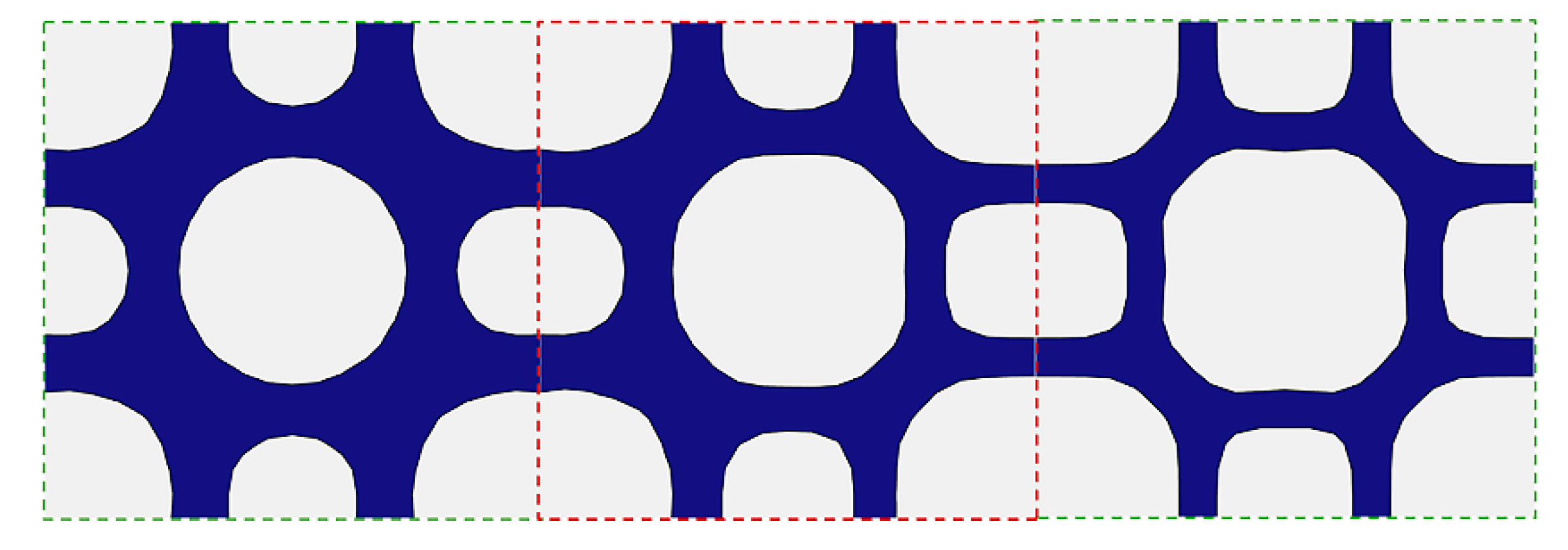
In order to ensure the smooth boundary, PLSM is adopted. Considering that the cellular structural boundary is embedded in the level set function $\mathsf{\Phi }(x)$, a specific level set determines the exact configuration of a cellular structure. Usually, for a periodic cellular structure, $\mathsf{\Phi }(x)$ is a square matrix, and the dimension is depended on the number of level set knots. To connect two adjacent cellular structures, a transitional cellular structure (TCS) can be generated via the interpolation of two level sets that respectively represent those two cellular structures. The constructed TCS can have partial features of both the adjacent cellular structures, so as to better fit the continuous change between different boundaries. 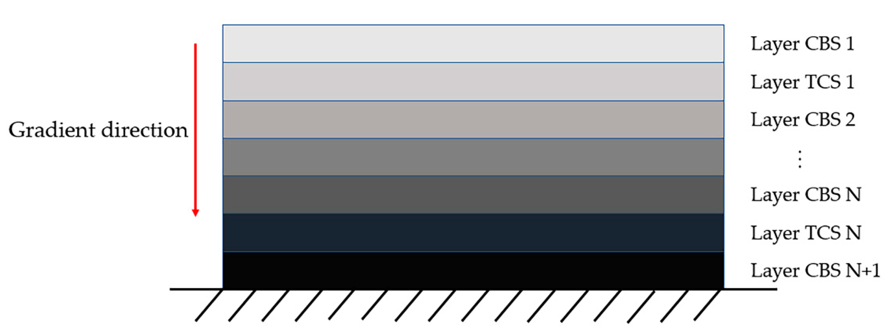A C¹ connection between gradient microstructures by using the proposed method is shown in Figure 2. Through the proposed method, the mismatch phenomenon can be completely avoided. To design the layer-wise FGM, this study creates a TCS between every two CBS over layers to maintain the C¹ connection. The macro configuration of the concerned FGM is shown in Figure 3, where every two CBS layers contain a transitional connecting TCS layer.

To construct a TCS, the corresponding level set functions of two optimized CBS are required. Different from the existing work, the $\mathsf{\Phi }(x)$ of TCS is not optimized but numerically interpolated. Thus, the level set function $\mathsf{\Phi }(x)$ of TCS can be obtained by using a very small computational effort. The interpolation process for TCS can be mathematically expressed as:

$${\mathsf{\Phi }}_{trans}(i)=(1-\beta (i))\cdot {\mathsf{\Phi }}_1(i)+\beta (i)\cdot {\mathsf{\Phi }}_2(i)(i=1,2...n)$$

(19)

where ${\mathsf{\Phi }}_{trans}$ is the level set function of the TCS. ${\mathsf{\Phi }}_1$ and ${\mathsf{\Phi }}_2$ respectively represent the level set function of the left and right CBS in Figure 2. n is the number of columns in the matrix of the level set function. $\beta$ is a weighting factor reflecting the degree of transition from left to right. In the interpolation process, the parameter $\beta$, which is a continuously changing value from 0 to 1, governs the geometry varying process from one CBS to the other CBS. Considering all the CBS in the FGM design, a transition cell can be easily constructed by using the level set functions of every two adjacent CBS. Therefore, the geometric continuity between two layers of the FGM can reach up to C¹. More importantly, the construction of every TCS in a cellular FGM has nothing to do with the optimization for the CBS. This means the CBS can be topologically designed without considering the connectivity constraints, and the performances of all the CBS will not be affected.

4. Numerical Examples in 2D Case

Generally, when considering the stiffness of a cellular structure, the bulk modulus and shear modulus are two main key properties to take into consideration [10]. In this section, to verify the validity of the proposed method, a family of CBS with maximum bulk modulus or shear modulus is firstly optimized with the volume fraction gradient change. Then, a series of TCS between every two CBS is interpolated, and the perfect connection state with C¹ smoothness is achieved by using the proposed transitional connection method.

In this study, the material properties of the CBS are reflected by the elasticity tensor $D^H$. For the topological optimization of CBS with extreme performances (i.e., maximum shear and bulk modulus) in 2D case, the objective function can be respectively established as follows:

$$J=\max D_{33}^H$$

(20)

$$J=\max \frac{1}{4}{\displaystyle \sum _{i,j}^2{D}_{i,j}^H}$$

(21)

Similarly, in the 3D case:

$$J=\max \frac{1}{3}(D_{44}^H+D_{55}^H+D_{66}^H)$$

(22)

$$J=\max \frac{1}{9}{\displaystyle \sum _{i,j=1}^3{D}_{i,j}^H}$$

(23)

4.1. Comparison of FGMs with C⁰ and C¹ Smoothness

For comparison, two different gradient connection methods are considered to construct the FGM, where the interfaces between different CBSs are respectively characterized with C⁰ and C¹ smoothness. First of all, FGM is devised by using the proposed transitional cell method, in which the FGM is consisting of CBSs and TCSs. Here, CBSs are optimized with the extreme performance of maximum bulk modulus, and the property gradient is governed by the gradually changing volume fraction along the predefined direction. In this example, each CBS is discretized into $20\times 20$ four-node quadrilateral elements. The Young’s modulus and Poisson’s ratio of the solid material are set as $\mathrm{E}=910\mathrm{MPa}$ and $\nu =0.3$, while in case of computational singularity, for the void material, ${\mathrm{E}}_{\mathrm{void}}=0.001\mathrm{MPa}$ and ${\nu }_{\mathrm{void}}=0.3$. The volume fraction of each CBS and TCS are displayed in

Table 1. Volume fraction of each cellular structure in Figure 4 (from left to right).

Serial Number	CBS 1	TCS 1	CBS 2	TCS 2	CBS 3
Volume fraction	0.25	0.3	0.35	0.4	0.45

. The optimized FGM with the specified gradient in volume fraction is presented in Figure 4. With the construction of transition cells, a smooth connection is achieved between the neighboring cellular structures. At the same time, the required characteristic of the volume fraction gradient is maintained.

Under the condition that each layer of the cellular structures in the FGM has the same volume fraction, the conventional FGM constituted by C⁰ connection is designed. In particular, the FGM with C⁰ connection can be implemented by respectively devising the CBSs with the corresponding gradient volume constraints. Then, the tailored CBSs are resembled along the gradient direction without constructing the TCS layers. In order to compare the effects of the two gradient connection methods on the structural mechanical properties, statics analysis in ANSYS Workbench is conducted. To ensure the validity of simulation, the gradient structure is tiled into 9 columns (Figure 5) and modelled with 1 mm thickness. The loading and boundary conditions are shown in Figure 6, where the bottom of the structure fixed and a set of uniformly distributed forces F = 20 N is applied at the top. The Young’s modulus and Poisson’s ratio of the solid material are set to be the same with the optimization configurations.

The simulation results are plotted in Figure 7, where the stresses on two selected joints in both the FGMs obtained by considering different interface smoothness are displayed. For the design with the C⁰ connection, the magnitude of the stresses is 5.9 MPa and 12.7 MPa. While for the design with C¹ smoothness, the magnitude of the stresses is 3.6 MPa and 5.9 MPa at the same sample points. From the results of the simulation analysis, it can be clearly seen that with the force applying on the top, the obvious stress concentration occurs at the interface between two adjacent cellular structures. When comparing to the result obtained by using the proposed transitional connection method, conventional FGM design with C⁰ connection displayed more serious stress concentration. Because the C⁰ connection only ensures that the similar CBSs can be connected, the connected interface lacks a smooth transition. In such a case, the connection surfaces in the FGM with C⁰ connection will be more likely to collapse. This proves that the proposed method can guarantee the higher-order continuity at the interfaces between the optimized CBSs, and thus alleviate the stress concentration at those interfaces.

In this study, the strain energy caused by the applied loads is selected as an indicator to illustrate the structural stiffness of the devised FGM. In other words, the smaller internal strain energy of a structure is, the better structural stiffness it will be [41]. For the two different FGM designs, the strain energy generated inside the structure is shown in

Table 2. Strain energy in simulations.

Connection Methods	C0 Connection	C1 Connection
Strain energy (mJ)	3.12	2.85

. The results show that the relative difference in the FGM with different connection methods is 8.65%, which means the proposed transitional connection method can also greatly increase the stiffness of the optimized FGM.

4.2. FGM with Maximum Bulk Modulus CBS

Section 4.1 illustrates that the FGM devised by using the transitional connection method can show the greater structural mechanical performances. In this section, the FGM design is compared to the design with uniformly shaped CBS. Here, the FGM with a smaller volume fraction gradient is considered. Each single cellular structure is discretized with 20 × 20 four-node quadrilateral elements, and the material properties are selected as $\mathrm{E}=910\mathrm{MPa}$ and $\nu =0.3$. The optimization objective of each CBS is the maximum bulk modulus. For comparison, the conventional porous structure with a single type CBS is also devised, under the same total volume constraint as well as the identical objective function. Two design results are shown in Figure 8, and the volume fraction of each CBS or TCS is shown in

Table 3. Volume fraction of cellular structure in Figure 8 (from left to right).

Cell Number	CBS 1	TCS 1	CBS 2	TCS 2	CBS 3	TCS 3	CBS 4
Volume fraction of each cell in Figure 8a	0.25	0.274	0.3	0.325	0.35	0.376	0.4
Volume fraction of each cell in Figure 8b	0.325	0.325	0.325	0.325	0.325	0.325	0.325

.

For the convenience of simulated analysis, two design results are tiled into 11 columns, and modelled with 1 mm thickness. For comparison, three different loading and boundary conditions are investigated, as shown in Figure 9. The magnitude of all the forces in the examples is set to be F = 50 N. Figure 10 shows the structure deformation within the two types of designs under the cantilever beam type condition. The strain energy under different loading and boundary conditions is compared in Figure 11. The improvement in structural stiffness of the FGM design when compared to the design with a single type CBS is also presented in

Table 4. The improvement on structural stiffness of the FGM design comparing to the design with single type CBS.

Loading Condition	Cantilever Beam	MBB Beam	Loading on Top
Performance improvement (%)	10.6	15.8	21

. The results clearly indicate that, under three common boundary conditions, the FGM design always performs better than the design with a single type CBS. It implies that the gradient structure can improve the mechanical performance. It is worth nothing that in some particular loading cases, the total deformation of FGM designs might be worse than that of the designs with uniform structures. In this case, the FGM design should be achieved by considering the coupling between macro and micro scales. However, this is beyond the scope of this study.

4.3. FGM with Maximum Shear Modulus CBS

In this example, CBS with extreme performance of maximum shear modulus is adopted for the design of FGM. Identically, the transitional connection method is used for the smooth connection of the microstructural boundary. The gradient of volume fraction is varying from 0.25 to 0.4. Each single cell is discretized by $20\times 20$ four-node quadrilateral elements, and the material properties are selected as $\mathrm{E}=910\mathrm{MPa}$ and $\nu =0.3$. Similarly, for comparison, the conventional porous structure with single type CBS is devised with the same total volume fraction. Two design results are shown in Figure 12, and the volume fraction of each CBS or TCS is shown in

Table 5. Volume fraction of cellular structure in Figure 12 (from left to right).

Cell Number	CBS 1	TCS 1	CBS 2	TCS 2	CBS 3	TCS 3	CBS 4
Volume fraction of each cell in Figure 12a	0.25	0.274	0.3	0.325	0.35	0.376	0.4
Volume fraction of each cell in Figure 12b	0.325	0.325	0.325	0.325	0.325	0.325	0.325

.

In the simulation analysis, the FGM is tiled into 11 columns, and modelled with 1 mm thickness. Similarly, three common boundary conditions given in Figure 9 are considered. The magnitude of all the forces in the examples is set to be 50 N, and the material properties in the simulation process are exactly the same as those in the optimization process. Figure 13 shows the structure deformation within the two designs under the same loading case of the cantilever beam type. The strain energy under different loading and boundary conditions is compared in Figure 14. The improvement in structural stiffness of the FGM design when compared to the design with a single type CBS is also presented in

Table 6. The improvement on structural stiffness of the FGM design comparing to the design with single type CBS.

Loading Condition	Cantilever Beam	MBB Beam	Loading on Top
Performance improvement (%)	8.8%	13.9%	25%

. It can be seen from the numerical results that, with the transitional connection, the FGM with maximum shear modulus CBS also shows a greater stiffness under the three different loading and boundary conditions.

4.4. FGM with Hybrid CBS

The rapid development of additive manufacturing promotes the design of complex structures. Another form of functionally gradient materials is the variation in the type of CBSs. For different type of CBSs, the discrepancy in both the shape and topology is even more obvious. As a result, the boundary mismatches are more prominent. What is worse, there are cases that two adjacent cellular structures are too different in their configurations to be able to connect. Fortunately, the proposed method can also be used to solve the smooth connection between different types of cellular structures.

Here, two different design methods are compared: one is to directly assemble the two types of cellular structures, the other is to use the proposed connection method to realize the smooth connection between the two types of cellular structures. In particular, two types of CBSs are optimized, i.e., the CBS with maximum bulk modulus and the CBS with maximum shear modulus. The volume fraction of every CBS is chosen as 0.35. Two FGM designs that are consisting of two different types of CBSs are shown in Figure 15. The constructed transitional cellular structure in Figure 15b shows the geometric features of both the two CBSs, which clearly illustrates the process of transition from one type of CBS to another type of CBS. It is obvious that the FGM in Figure 15b has a smooth boundary between two different types of CBSs. Thus, it can greatly facilitate the manufacturing process and a decrease in stress concentration is expected.

5. Numerical Examples in 3D Case

To demonstrate the proposed method for the design of 3D FGM, this example gives several 3D FGM with a volume fraction gradient. The 3D CBSs are optimized with maximum bulk modulus and maximum shear modulus. Each of the cellular structure is discretized with $20\times 20\times 20$ eight-node cubic elements. The Young’s modulus and Poisson’s ratio of the solid material in the optimization are selected as $\mathrm{E}=\mathrm{10,000}\mathrm{MPa}$ and $\nu =0.3$. The Young’s modulus and Poisson’s ratio for the void part in the optimization are ${\mathrm{E}}_{\mathrm{void}}=0.001\mathrm{MPa}$ and ${\nu }_{\mathrm{void}}=0.3$. In the same way, the 3D transitional cellular structures are constructed using the proposed method. The 3D FGM with two different extreme performances CBS are shown in Figure 16, and the volume fraction of each CBS or TCS are shown in

Table 7. Volume fraction of each cellular structure in Figure 16 (from left to right).

Cell Number	CBS 1	TCS 1	CBS 2	TCS 2	CBS 3
Volume fraction of each cell in Figure 16a	0.325	0.337	0.35	0.363	0.375
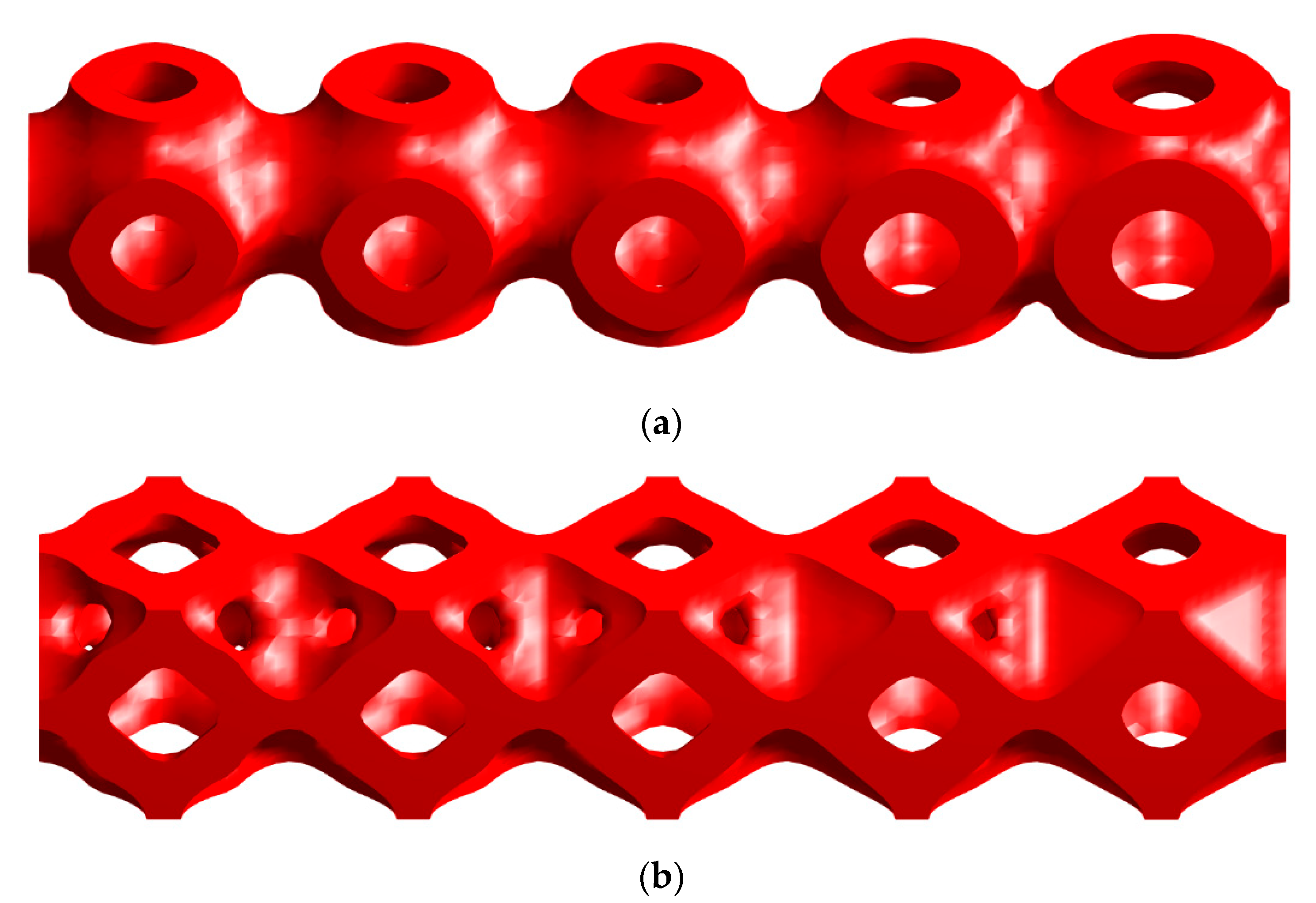
Volume fraction of each cell in Figure 16b	0.325	0.337	0.35	0.362	0.375

. The design results show that the boundaries between different cellular structures can be connected smoothly. From the connection modality, it clearly demonstrates that the proposed transitional connection method also applies to the 3D case.

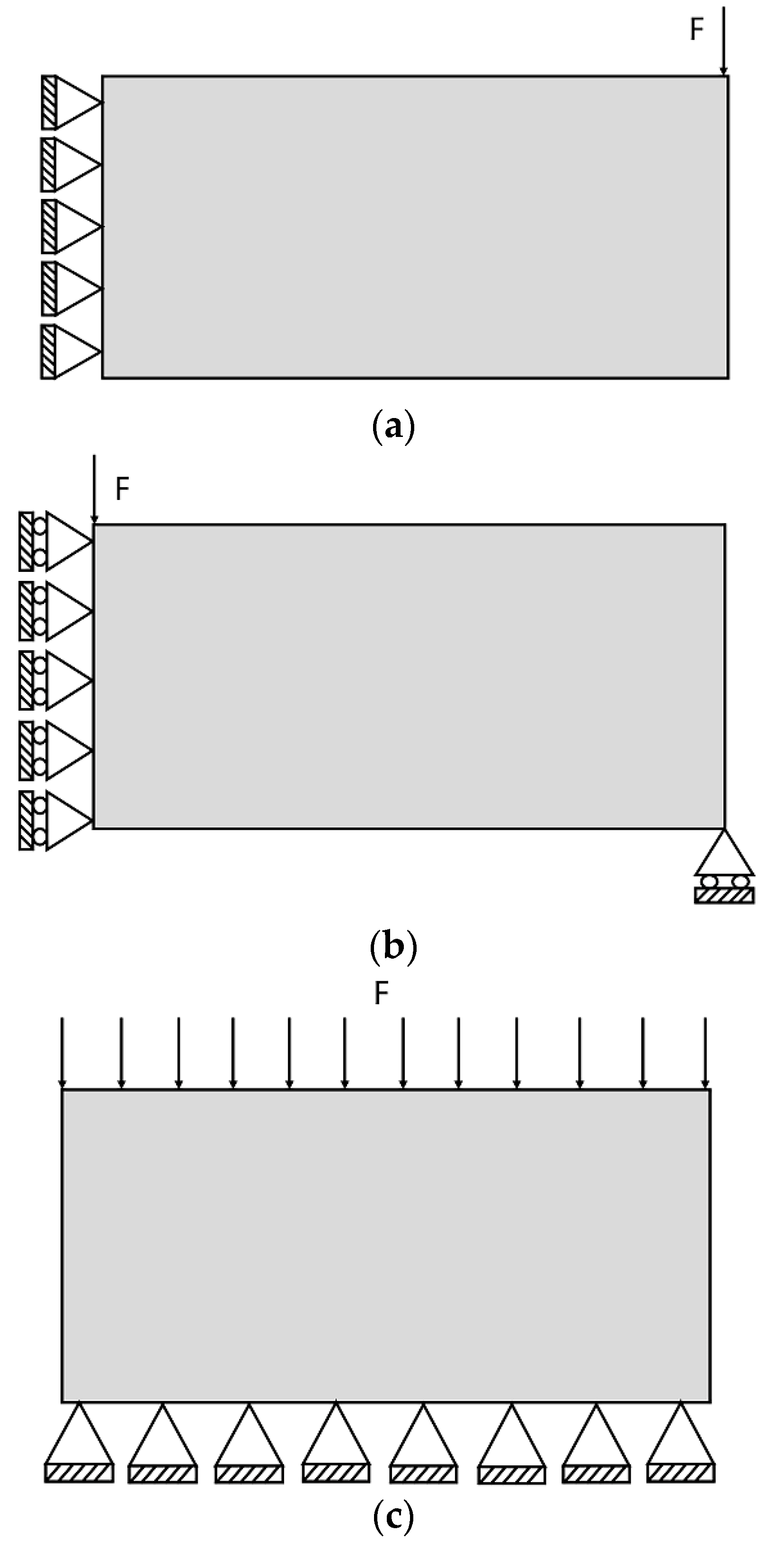
For comparison, the porous structure with a single type 3D maximum shear modulus CBS is also devised. The volume fraction of every single CBS is selected as 0.35, which ensures the total volume fraction of the design is exactly the same as that of the FGM design in Figure 16b. The optimized porous structure with a single type 3D maximum shear modulus CBS is shown in Figure 17. The comparative analysis of the mechanical properties is implemented in ANSYS Workbench. The two designs are arrayed in a 5 × 5 structure. The loading and boundary conditions are presented in Figure 18, and the magnitude of the force is set to be 10 kN. 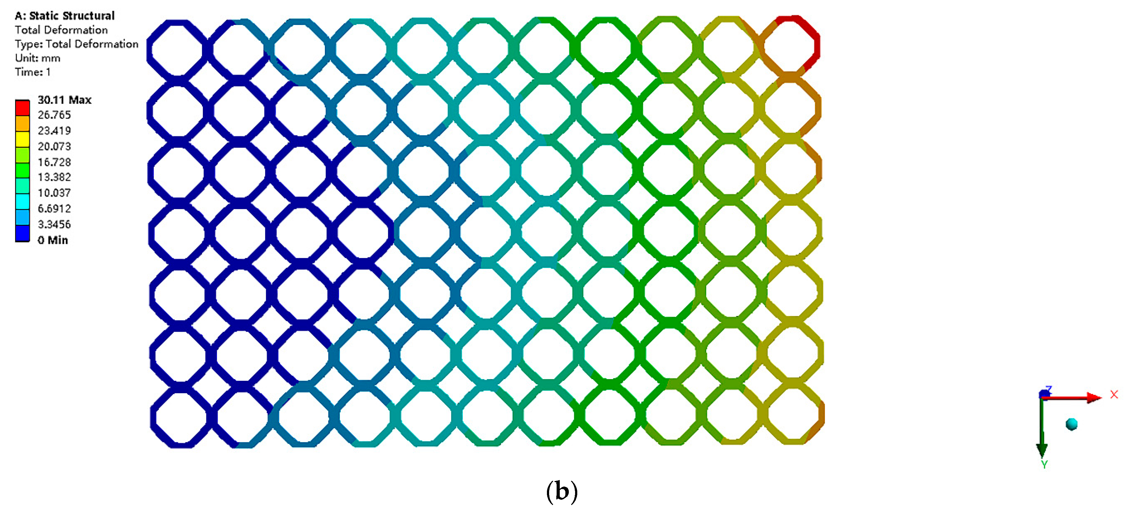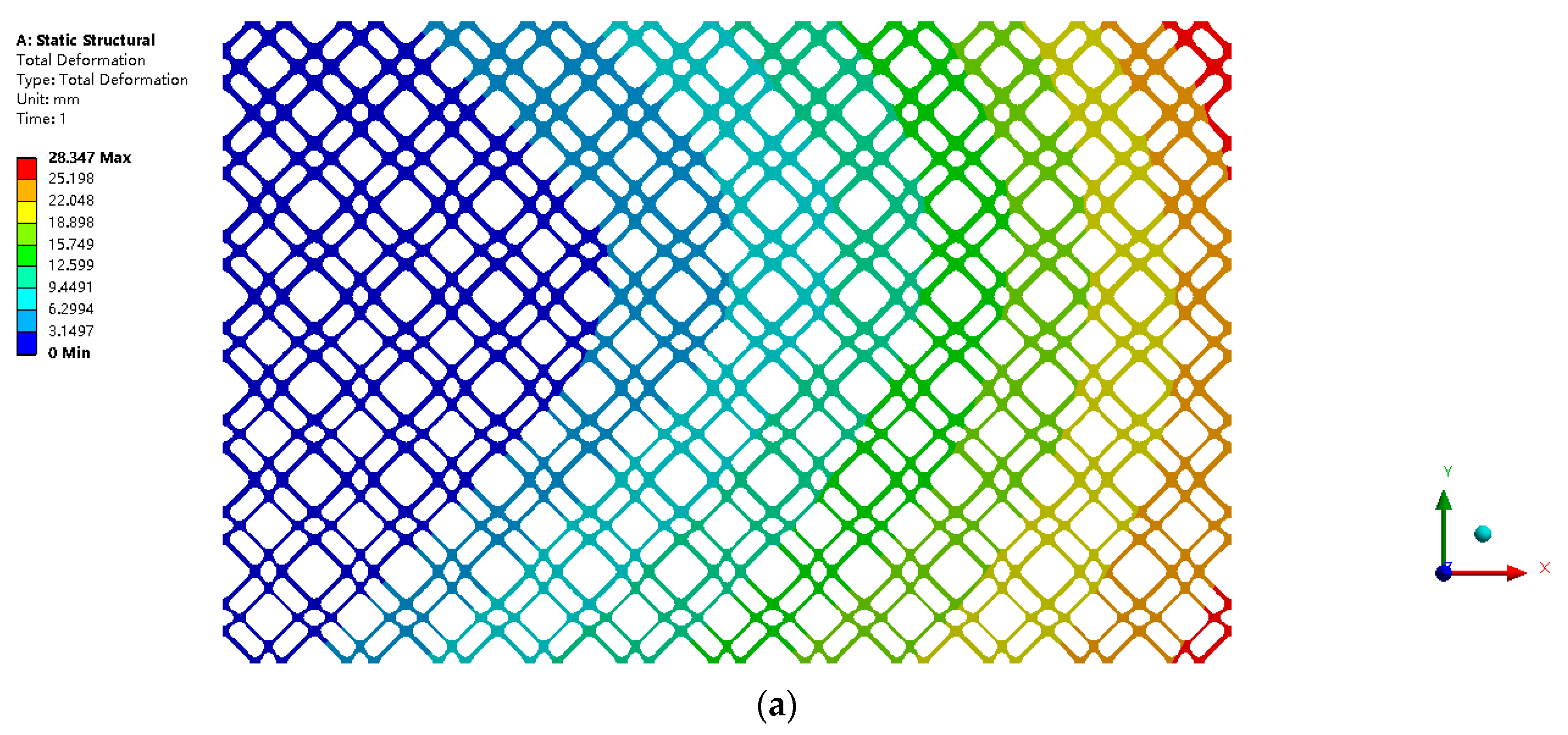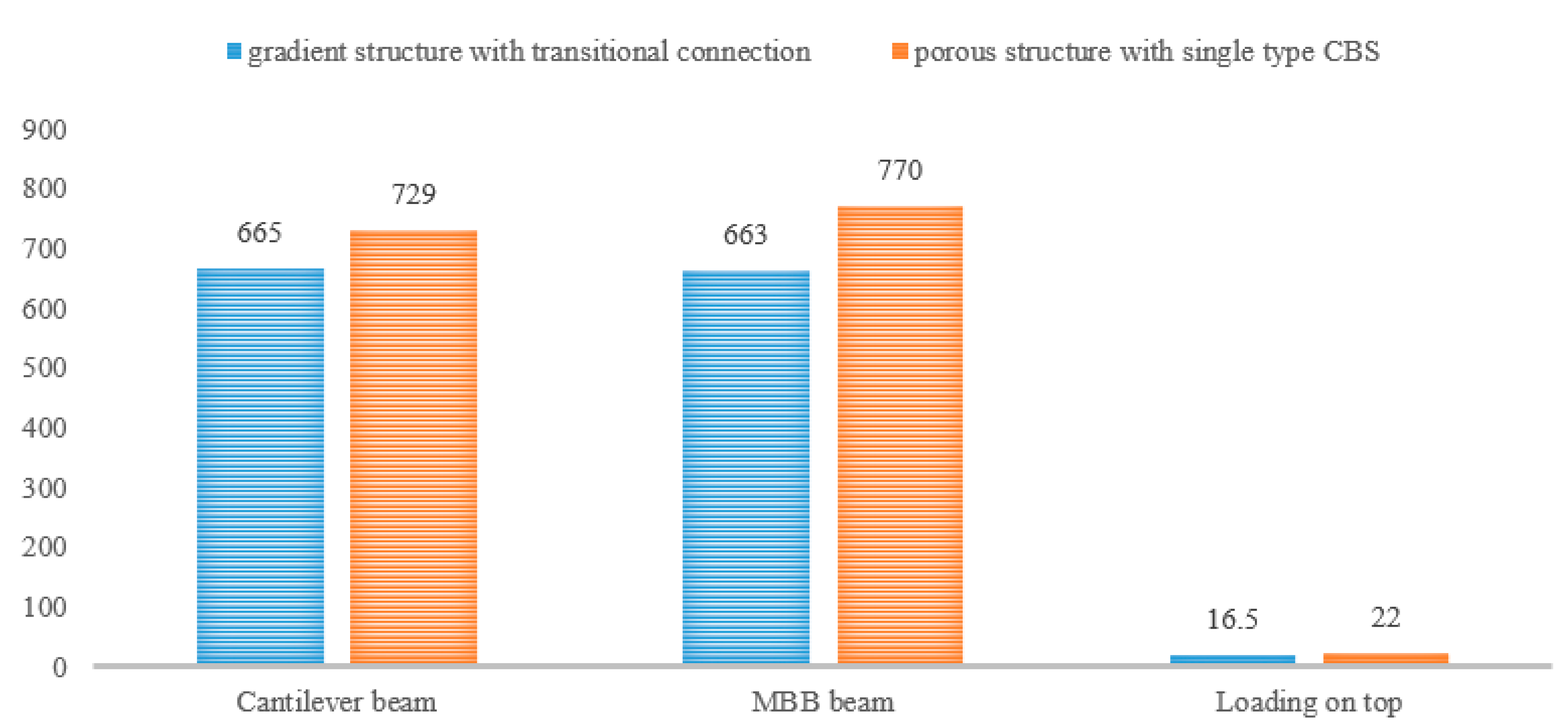Figure 19 displays the structural deformation within the two types of structures under the same loading and boundary conditions. Identically, the strain energy is chosen as a reference to evaluate the structural stiffness. The strain energy for different designs is given in the

Table 8. Strain energy for the 3D cases.

Type of Design	FGM	Design with Single Type CBS
Strain energy(mJ)	449	468

. The simulation results showed that the FGM design can perform better than the design with a single type of CBS in the 3D scenario. It implies that the gradient structure can also improve the mechanical performance in the 3D case. Particularly, in this study, the volume fraction is selected as the key parameter to induce the gradient property. The TCS can ensure a precise control on its volume fraction, which is highly related to its structural stiffness. However, the proposed approach relies uniquely on pure geometrical considerations, and it is restricted to the design of the layer-wise cellular FGMs. Although we use the strain energy to evaluate the performance of the FGMs, the proposed method does not consider the strong coupling on the macro and micro scales. A future extension of this approach will be the solution of multiscale design for the FGMs with C¹ connection.

In addition, the proposed transitional connection method is also applied to the design of 3D FGM with different types of CBSs. In this example, two types of CBSs are considered, including the CBS with maximum bulk modulus and the CBS with maximum shear modulus. The final design is presented in Figure 20. To make the structure joints more visible, the configuration of transitional cellular structure is exhibited in Figure 21 with different views. On both sides of the transitional cellular structure, its surface shape is the same with that of the connected cellular structures, so the geometry of different cells can fit perfectly. Figure 22 shows a sectional view. It can be seen that the transitional cellular structure has the geometric features of both CBSs. Therefore, even in the 3D cases, the transitional connection method can be used to tackle the different types of CBSs, so as to guarantee a smooth interface between adjacent cells in the cellular FGMs.

6. Conclusions

This paper proposes a transitional connection method for the optimization design of FGMs. Based on the parametric level set method, the configuration of every cellular based cell is represented by a specific level set function. For every two gradient base cells in a FGM, a special transitional cell is constructed using the two level set functions of two candidate base cells. Since the transitional cell has the geometric features of two gradient base cells, the shape of the transitional cell fits perfectly with its connected gradient cells on both sides. Thus, the FGM design can have smooth connectivity with C¹ continuity. In particular, the interpolation of the transitional cell independent of the optimization avoids added computing time.

To validate the proposed method for devising the FGMs, several 2D and 3D examples are provided. In addition, a series of comparative simulation analyses are carried out. Firstly, a number of FGM designs obtained by using the proposed connection method exhibit smooth interfaces between different layers. Secondly, simulation results demonstrate the advantages of the proposed method over the direct connection method to alleviate the stress concentration in the design. Thirdly, compared to the conventional porous structure with single type CBS, when the structural strain energy is taken as a reference, the devised gradient structure can exhibit better structural stiffness. Finally, for the FGM with different types of CBSs, the proposed method can be effectively used to solve the boundary mismatches. The optimization design process and the comparative simulation analysis indicate the easiness and effectiveness of the proposed method. Note that the proposed method is developed under the assumption that the material microstructures are with the plane symmetry. The more general elastic symmetries (e.g., tetragonal or monoclinic symmetries) are also quite important and worth a comprehensive investigation. In that case, the approach based on tensor invariants can be adopted [55,56]. The consideration of general elastic symmetries can be a future extension of the proposed method.

References

1. Sarkar, P.; Bosneaga, E.; Auer, M. Plant cell walls throughout evolution: Towards a molecular understanding of their design principles. J. Exp. Bot. 2009, 60, 3615–3635. [Google Scholar] [CrossRef] [PubMed] [Green Version]
2. Silva, E.C.N.; Walters, M.C.; Paulino, G.H. Modeling bamboo as a functionally graded material: Lessons for the analysis of affordable materials. J. Mater. Sci. 2006, 41, 6991–7004. [Google Scholar] [CrossRef]
3. Zheng, X.; Lee, H.; Weisgraber, T.H.; Shusteff, M.; DeOtte, J.; Duoss, E.B.; Kuntz, J.D.; Biener, M.M.; Ge, Q.; Jackson, J.A.; et al. Ultralight, ultrastiff mechanical metamaterials. Science 2014, 344, 1373. [Google Scholar] [CrossRef] [PubMed] [Green Version]
4. Valdevit, L.; Jacobsen, A.J.; Greer, J.R.; Carter, W.B. Protocols for the Optimal Design of Multi-Functional Cellular Structures: From Hypersonics to Micro-Architected Materials. J. Am. Ceram. Soc. 2011, 94, s15–s34. [Google Scholar] [CrossRef]
5. Christensen, R.M. Mechanics of cellular and other low-density materials. Int. J. Solids Struct. 2000, 37, 93–104. [Google Scholar] [CrossRef]
6. Meza, L.R.; Das, S.; Greer, J.R. Strong, lightweight, and recoverable three-dimensional ceramic nanolattices. Science 2014, 345, 1322. [Google Scholar] [CrossRef] [Green Version]
7. Olson , R.A., III; Martins, L.C.B. Cellular Ceramics in Metal Filtration. Adv. Eng. Mater. 2005, 7, 187–192. [Google Scholar] [CrossRef]
8. Li, H.; Gao, L.; Li, H.; Tong, H. Spatial-varying multi-phase infill design using density-based topology optimization. Comput. Methods Appl. Mech. Eng. 2020, 372, 113354. [Google Scholar] [CrossRef]
9. Zhou, S.; Li, Q. Design of graded two-phase microstructures for tailored elasticity gradients. J. Mater. Sci. 2008, 43, 5157–5167. [Google Scholar] [CrossRef]
10. Radman, A.; Huang, X.; Xie, Y.M. Topology optimization of functionally graded cellular materials. J. Mater. Sci. 2013, 48, 1503–1510. [Google Scholar] [CrossRef]
11. Cadman, J.E.; Zhou, S.; Chen, Y.; Li, Q. On design of multi-functional microstructural materials. J. Mater. Sci. 2013, 48, 51–66. [Google Scholar] [CrossRef]
12. Wang, Y.; Chen, F.; Wang, M.Y. Concurrent design with connectable graded microstructures. Comput. Methods Appl. Mech. Eng. 2017, 317, 84–101. [Google Scholar] [CrossRef]
13. Bendsøe, M.P.; Sigmund, O. Topology Optimization: Theory, Methods and Applications; Springer: Berlin/Heidelberg, Germany, 2003. [Google Scholar]
14. Bendsøe, M.P.; Kikuchi, N. Generating optimal topologies in structural design using a homogenization method. Comput. Methods Appl. Mech. Eng. 1988, 71, 197–224. [Google Scholar] [CrossRef]
15. Sigmund, O. A 99 line topology optimization code written in Matlab. Struct. Multidiscip. Optim. 2001, 21, 120–127. [Google Scholar] [CrossRef]
16. Bendsøe, M.P.; Sigmund, O. Material interpolation schemes in topology optimization. Arch. Appl. Mech. 1999, 69, 635–654. [Google Scholar] [CrossRef]
17. Xie, Y.M.; Steven, G.P. A simple evolutionary procedure for structural optimization. Comput. Struct. 1993, 49, 885–896. [Google Scholar] [CrossRef]
18. Huang, X.; Xie, Y.M. Bi-directional evolutionary topology optimization of continuum structures with one or multiple materials. Comput. Mech. 2008, 43, 393. [Google Scholar] [CrossRef]
19. Sethian, J.A.; Wiegmann, A. Structural boundary design via level set and immersed interface methods. J. Comput. Phys. 2000, 163, 489–528. [Google Scholar] [CrossRef]
20. Wang, M.Y.; Wang, X.M.; Guo, D.M. A level set method for structural topology optimization. Comput. Methods Appl. Mech. Eng. 2003, 192, 227–246. [Google Scholar] [CrossRef]
21. Allaire, G.; Jouve, F.; Toader, A.-M. Structural optimization using sensitivity analysis and a level-set method. J. Comput. Phys. 2004, 194, 363–393. [Google Scholar] [CrossRef] [Green Version]
22. van Dijk, N.P.; Maute, K.; Langelaar, M.; van Keulen, F. Level-set methods for structural topology optimization: A review. Struct. Multidiscip. Optim. 2013, 48, 437–472. [Google Scholar] [CrossRef]
23. Costa, G.; Montemurro, M.; Pailhès, J. A 2D topology optimisation algorithm in NURBS framework with geometric constraints. Int. J. Mech. Mater. Des. 2018, 14, 669–696. [Google Scholar] [CrossRef] [Green Version]
24. Costa, G.; Montemurro, M.; Pailhès, J. NURBS hyper-surfaces for 3D topology optimization problems. Mech. Adv. Mater. Struct. 2019, 1–20. [Google Scholar] [CrossRef]
25. Costa, G.; Montemurro, M.; Pailhès, J. Minimum length scale control in a NURBS-based SIMP method. Comput. Methods Appl. Mech. Eng. 2019, 354, 963–989. [Google Scholar] [CrossRef]
26. Andreassen, E.; Andreasen, C.S. How to determine composite material properties using numerical homogenization. Comput. Mater. Sci. 2014, 83, 488–495. [Google Scholar] [CrossRef] [Green Version]
27. Sigmund, O. A new class of extremal composites. J. Mech. Phys. Solids 2000, 48, 397–428. [Google Scholar] [CrossRef]
28. Wang, Y.; Luo, Z.; Zhang, N.; Kang, Z. Topological shape optimization of microstructural metamaterials using a level set method. Comput. Mater. Sci. 2014, 87, 178–186. [Google Scholar] [CrossRef]
29. Ye, M.; Gao, L.; Li, H. A design framework for gradually stiffer mechanical metamaterial induced by negative Poisson’s ratio property. Mater. Des. 2020, 192, 108751. [Google Scholar] [CrossRef]
30. Zhang, H.; Wang, Y.; Kang, Z. Topology optimization for concurrent design of layer-wise graded lattice materials and structures. Int. J. Eng. Sci. 2019, 138, 26–49. [Google Scholar] [CrossRef]
31. Li, H.; Li, H.; Xiao, M.; Zhang, Y.; Fu, J.; Gao, L. Robust topology optimization of thermoelastic metamaterials considering hybrid uncertainties of material property. Compos. Struct. 2020, 248, 112477. [Google Scholar] [CrossRef]
32. Sigmund, O. Materials with prescribed constitutive parameters: An inverse homogenization problem. Int. J. Solids Struct. 1994, 31, 2313–2329. [Google Scholar] [CrossRef]
33. Radman, A.; Huang, X.; Xie, Y.M. Topological optimization for the design of microstructures of isotropic cellular materials. Eng. Optim. 2013, 45, 1331–1348. [Google Scholar] [CrossRef]
34. Vatanabe, S.L.; Paulino, G.H.; Silva, E.C.N. Design of functionally graded piezocomposites using topology optimization and homogenization—Toward effective energy harvesting materials. Comput. Methods Appl. Mech. Eng. 2013, 266, 205–218. [Google Scholar] [CrossRef]
35. Koizumi, M. FGM activities in Japan. Compos. Part B Eng. 1997, 28, 1–4. [Google Scholar] [CrossRef]
36. Sigmund, O.; Torquato, S. Design of Materials with Extreme Elastic or Thermoelastic Properties Using Topology Optimization. In IUTAM Symposium on Transformation Problems in Composite and Active Materials. Solid Mechanics and its Applications; Springer: Dordrecht, The Netherlands, 1998. [Google Scholar]
37. Diaz, A.R.; Sigmund, O. A topology optimization method for design of negative permeability metamaterials. Struct. Multidiscip. Optim. 2010, 41, 163–177. [Google Scholar] [CrossRef]
38. Gao, J.; Li, H.; Luo, Z.; Gao, L.; Li, P. Topology Optimization of Micro-Structured Materials Featured with the Specific Mechanical Properties. Int. J. Comput. Methods 2018, 17, 1850144. [Google Scholar] [CrossRef] [Green Version]
39. Challis, V.J.; Cramer, A.D.; Roberts, A.P. An optimised family of anisotropic microstructures with application to functionally graded materials. Int. J. Solids Struct. 2019, 171, 17–29. [Google Scholar] [CrossRef]
40. Garner, E.; Kolken, H.M.A.; Wang, C.C.L.; Zadpoor, A.A.; Wu, J. Compatibility in microstructural optimization for additive manufacturing. Addit. Manuf. 2019, 26, 65–75. [Google Scholar] [CrossRef]
41. Panesar, A.; Abdi, M.; Hickman, D.; Ashcroft, I. Strategies for functionally graded lattice structures derived using topology optimisation for Additive Manufacturing. Addit. Manuf. 2018, 19, 81–94. [Google Scholar] [CrossRef]
42. Zong, H.; Liu, H.; Ma, Q.; Tian, Y.; Zhou, M.; Wang, M.Y. VCUT level set method for topology optimization of functionally graded cellular structures. Comput. Methods Appl. Mech. Eng. 2019, 354, 487–505. [Google Scholar] [CrossRef]
43. Liu, H.; Zong, H.; Shi, T.; Xia, Q. M-VCUT level set method for optimizing cellular structures. Comput. Methods Appl. Mech. Eng. 2020, 367, 113154. [Google Scholar] [CrossRef]
44. Maskery, I.; Aremu, A.O.; Parry, L.; Wildman, R.D.; Tuck, C.J.; Ashcroft, I.A. Effective design and simulation of surface-based lattice structures featuring volume fraction and cell type grading. Mater. Des. 2018, 155, 220–232. [Google Scholar] [CrossRef]
45. Wei, P.; Li, Z.; Li, X.; Wang, M.Y. An 88-line MATLAB code for the parameterized level set method based topology optimization using radial basis functions. Struct. Multidiscip. Optim. 2018, 58, 831–849. [Google Scholar] [CrossRef]
46. Osher, S.; Sethian, J.A. Fronts propagating with curvature-dependent speed: Algorithms based on Hamilton-Jacobi formulations. J. Comput. Phys. 1988, 79, 12–49. [Google Scholar] [CrossRef] [Green Version]
47. Zhou, M.; Rozvany, G.I.N. The COC algorithm, Part II: Topological, geometrical and generalized shape optimization. Comput. Methods Appl. Mech. Eng. 1991, 89, 309–336. [Google Scholar] [CrossRef]
48. Svanberg, K. The Method of Moving Asymptotes (MMA) with Some Extensions. In Optimization of Large Structural Systems; Rozvany, G.I.N., Ed.; Springer: Dordrecht, The Netherlands, 1993; pp. 555–566. [Google Scholar]
49. Belytschko, T.; Xiao, S.; Parimi, C. Topology optimization with implicit functions and regularization. Int. J. Numer. Methods Eng. 2003, 57, 1177–1196. [Google Scholar] [CrossRef]
50. Li, H.; Li, P.; Gao, L.; Zhang, L.; Wu, T. A level set method for topological shape optimization of 3D structures with extrusion constraints. Comput. Methods Appl. Mech. Eng. 2015, 283, 615–635. [Google Scholar] [CrossRef]
51. Luo, Z.; Wang, M.; Wang, S.; Wei, P. A level set-based parameterization method for structural shape and topology optimization. Int. J. Numer. Methods Eng. 2008, 76, 1–26. [Google Scholar] [CrossRef]
52. Wendland, H. Piecewise polynomial, positive definite and compactly supported radial functions of minimal degree. Adv. Comput. Math. 1995, 4, 389–396. [Google Scholar] [CrossRef]
53. Daru, V. Level Set Methods and Fast Marching Methods—Evolving Interfaces in Computational Geometry, Fluid Mechanics, Computer Vision, and Materials Science, 2nd ed.; Sethian, J.A., Ed.; Cambridge University Press: Cambridge, UK, 1999; 378p. [Google Scholar]
54. Osher, S.; Fedkiw, R.P. Level Set Methods: An Overview and Some Recent Results. J. Comput. Phys. 2001, 169, 463–502. [Google Scholar] [CrossRef] [Green Version]
55. Catapano, A.; Montemurro, M. On the correlation between stiffness and strength properties of anisotropic laminates. Mech. Adv. Mater. Struct. 2017, 26, 651–660. [Google Scholar] [CrossRef] [Green Version]
56. Vannucci, P.; Desmorat, B. Plane anisotropic rari-constant materials. Math. Methods Appl. Sci. 2015, 39, 3271–3281. [Google Scholar] [CrossRef] [Green Version]
Figure 1. C0 connectivity in FGM.
Applsci 10 07449 g001
Figure 2. Transitional cell (middle) to connect two CBS (left and right) with C1 continuity.
Applsci 10 07449 g002
Figure 3. Configuration of the considered FGM.
Applsci 10 07449 g003
Figure 4. FGM with maximum bulk modulus cellular structure.
Applsci 10 07449 g004
Figure 5. Two different connection method for the design of FGM: (a) conventional FGM with C0 connection; (b) FGM with C1 connection by using the transitional connection method.
Applsci 10 07449 g005
Figure 6. Loading and boundary conditions for optimized FGMs in ANSYS simulation analysis.
Applsci 10 07449 g006
Figure 7. The stress distribution of optimized FGMs (specified gradient in volume fraction) with two different connection methods: (a) conventional FGM with C0 connection; (b) FGM with C1 connection by using the transitional connection method.
Applsci 10 07449 g007
Figure 8. Two different porous structures with the maximum bulk modulus: (a) FGM design; (b) design with single type CBS.
Applsci 10 07449 g008
Figure 9. Three different loading and boundary conditions: (a) cantilever beam; (b) half MBB beam; (c) Loading on top.
Applsci 10 07449 g009
Figure 10. Structural deformation under the cantilever beam type condition: (a) FGM design; (b) design with single type CBS.
Applsci 10 07449 g010aApplsci 10 07449 g010b
Figure 11. Strain energy comparison for two designs under different loading and boundary conditions.
Applsci 10 07449 g011
Figure 12. Two different porous structures with the maximum shear modulus: (a) FGM design; (b) design with single type CBS.
Applsci 10 07449 g012
Figure 13. Structural deformation under the cantilever beam type condition: (a) FGM design; (b) design with single type CBS.
Applsci 10 07449 g013aApplsci 10 07449 g013b
Figure 14. Strain energy comparison for two designs under different loading and boundary conditions.
Applsci 10 07449 g014
Figure 15. Designs with two connection methods: (a) FGM with mismatched interfaces by directly connecting the two types of CBSs; (b) FGM with smooth interfaces by using the transitional connection method.
Applsci 10 07449 g015
Figure 16. Two kinds of 3D FGM by using the proposed transitional connection method: (a) 3D FGM with maximum bulk modulus CBSs; (b) 3D FGM with maximum shear modulus CBSs.
Applsci 10 07449 g016
Figure 17. Porous structure with single type 3D maximum shear modulus CBS.
Applsci 10 07449 g017
Figure 18. Loading and boundary conditions for the 3D porous structure.
Applsci 10 07449 g018
Figure 19. Structural deformation under the considered loading and boundary conditions: (a) FGM design; (b) design with single type CBS.
Applsci 10 07449 g019aApplsci 10 07449 g019b
Figure 20. 3D FGM with smooth interfaces by using the transitional connection method.
Applsci 10 07449 g020
Figure 21. Different perspectives of the 3D transitional cellular structure: (a) perspective 1, top surface connects perfectly with the maximum shear modulus CBS; (b) perspective 2, top surface connects perfectly with the maximum bulk modulus CBS.
Applsci 10 07449 g021
Figure 22. Sectional view of the connection between different cells.
Applsci 10 07449 g022