Latency-Aware DU/CU Placement in Convergent Packet-Based 5G Fronthaul Transport Networks


Abstract
1. Introduction
1.1. Related Works
1.2. Contributions
- development of an MILP optimization model for latency-aware DU/CU placement;
- in the MILP model, consideration of three different traffic flows (FH, MH, BH) realized jointly in the NGFI network;
- in the MILP model, consideration of limited PP processing capacities in the NGFI network;
- reporting and discussion of results of numerical experiments assessing performance of the MILP optimization model proposed and evaluating NGFI network performance in different scenarios.
2. Network Model
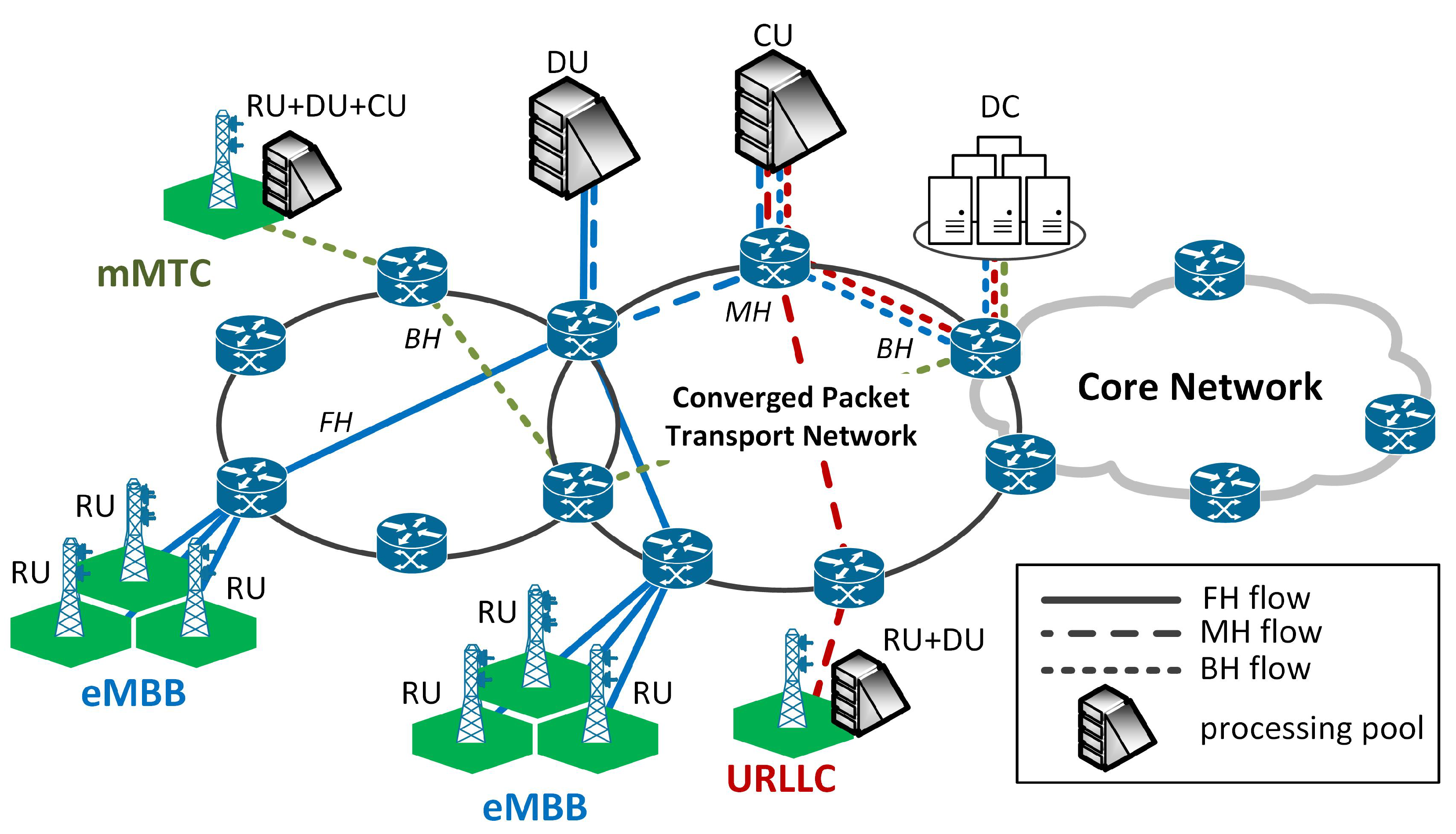
2.1. NGFI Network
2.2. Traffic Flows
2.3. Packet Transport Network
2.4. Traffic Model
2.5. Latencies Modeling
- propagation in links,
- storing and forwarding of frames in switches,
- transmission times of bursts of frames, and
- queuing of frames at output ports of switches.
- delay produced by the flows of either higher or equal priority (), and
- delay produced by lower priority flows ().
3. LDCP Problem
- placement (in selected PP nodes) of DU and CU entities realizing baseband processing functions for a set of RU nodes, assuming given constraints on
- maximum processing capacities of the PP nodes,
- maximum latencies of the fronthaul, midhaul, and backhaul flows realized over the packet transport network between the RUs, the PP nodes selected (for DU and CU processing), and the DC node, and
- allocation of bandwidth in network links so that to transport FH, MH, and BH flows, assuming given constraints on links capacities.
3.1. Notation
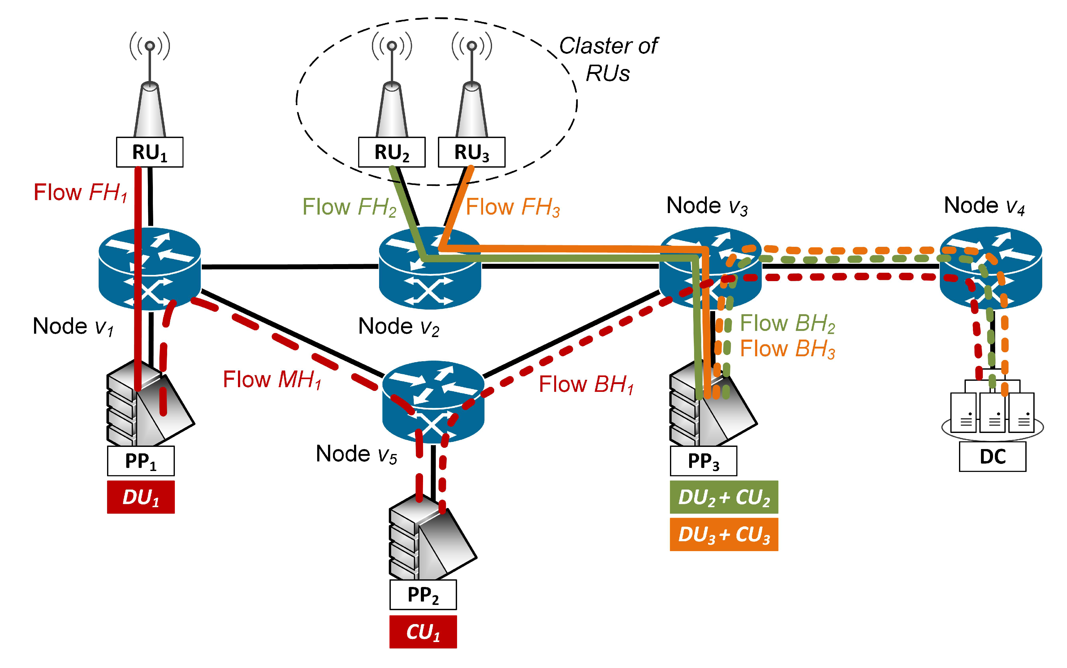
- a fronthaul flow—between the RU node and the PP node in which the DU entity is placed;
- a midhaul flow—between the PP node in which the DU entity is located and a different PP node in which the CU entity is placed. Note that if the DU and CU are located in the same PP node for a given demand, then the MH flow is not present in the network for this demand;
- a backhaul flow—between the PP node in which the CU entity is located and a DC node.
- if d is an uplink demand, then: and if , and if , and and if ;
- if d is a downlink demand, then: and if , and if , and and if .
3.2. Problem Statement
- Clustering of RUs: the DUs associated with the RUs that belong to the same cluster are placed in the same PP node;
- PP node assignment for DU processing: for each demand, locate the DU in the PP node that has been assigned to its cluster (i.e., to which its RU belongs to);
- PP node selection for CU processing: a PP node is selected for the CU processing of the demand;
- PP node capacity: the overall DU and CU processing load of all demands processed in each PP node does not exceed the node processing capacity;
- Traffic flows: the traffic flows (FH, MH, and BH) are terminated in the PP nodes in which DU and CU entities are placed; if DU and CU are located in the same PP node, then flow MH is not realized in the network;
- Capacity of link: the overall bit-rates of all flows going through a link must be lower or equal to the link capacity;
- Latency of flow: the latency of a flow cannot be greater than the maximum latency that is allowable for this flow.
3.3. MILP Formulation
4. Numerical Results
4.1. Performance of LDCP-MILP Model
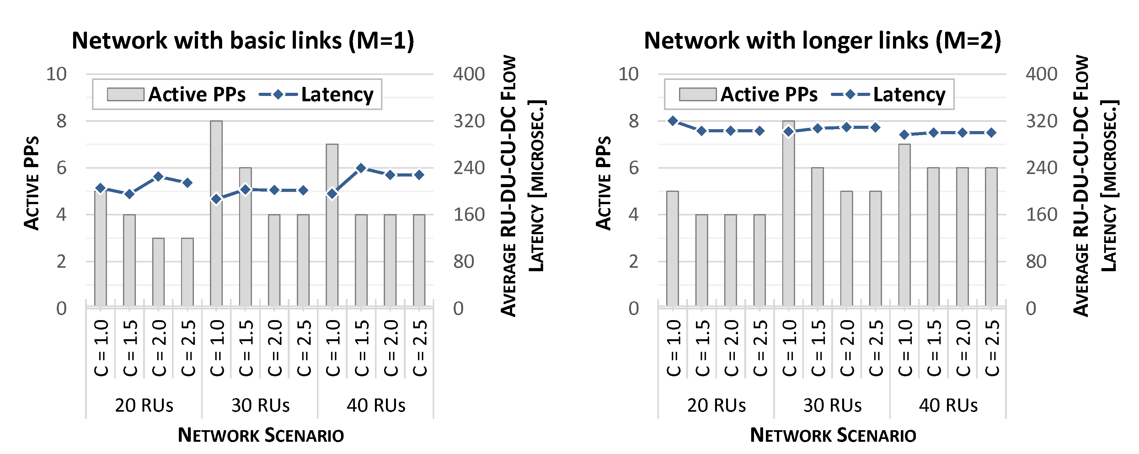
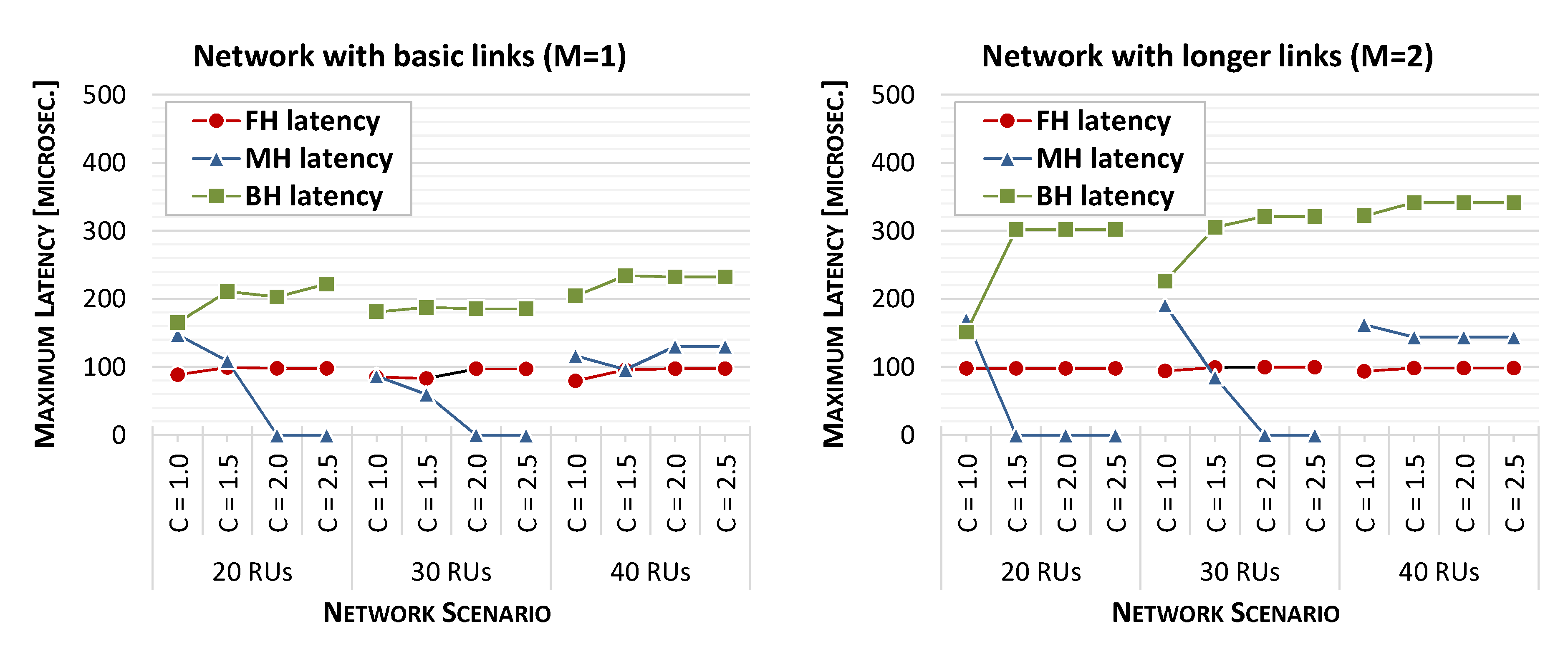
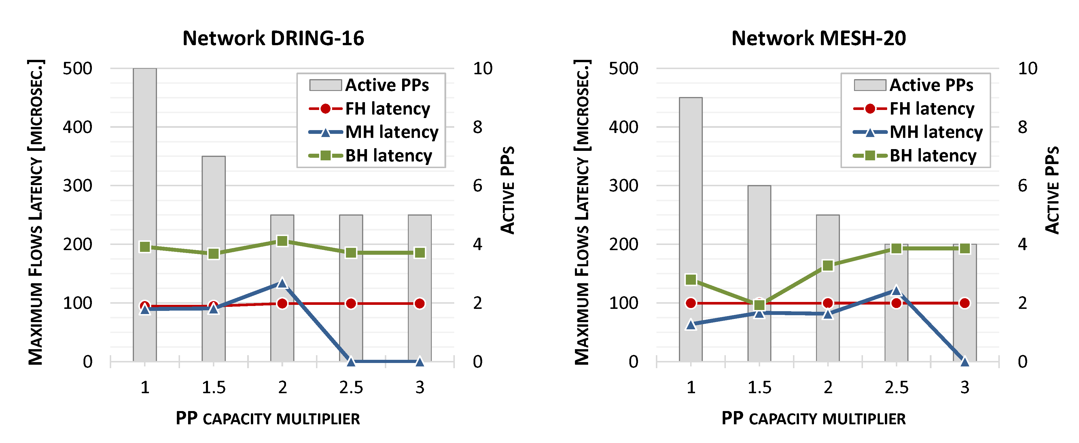
4.2. Analysis of Network Performance
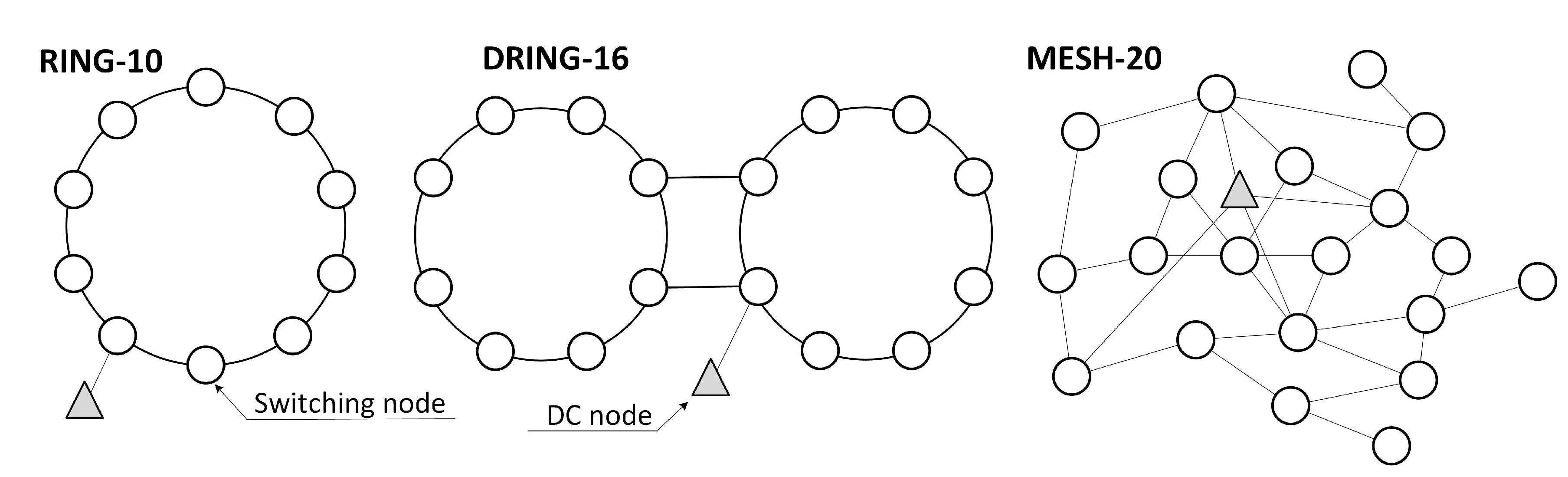
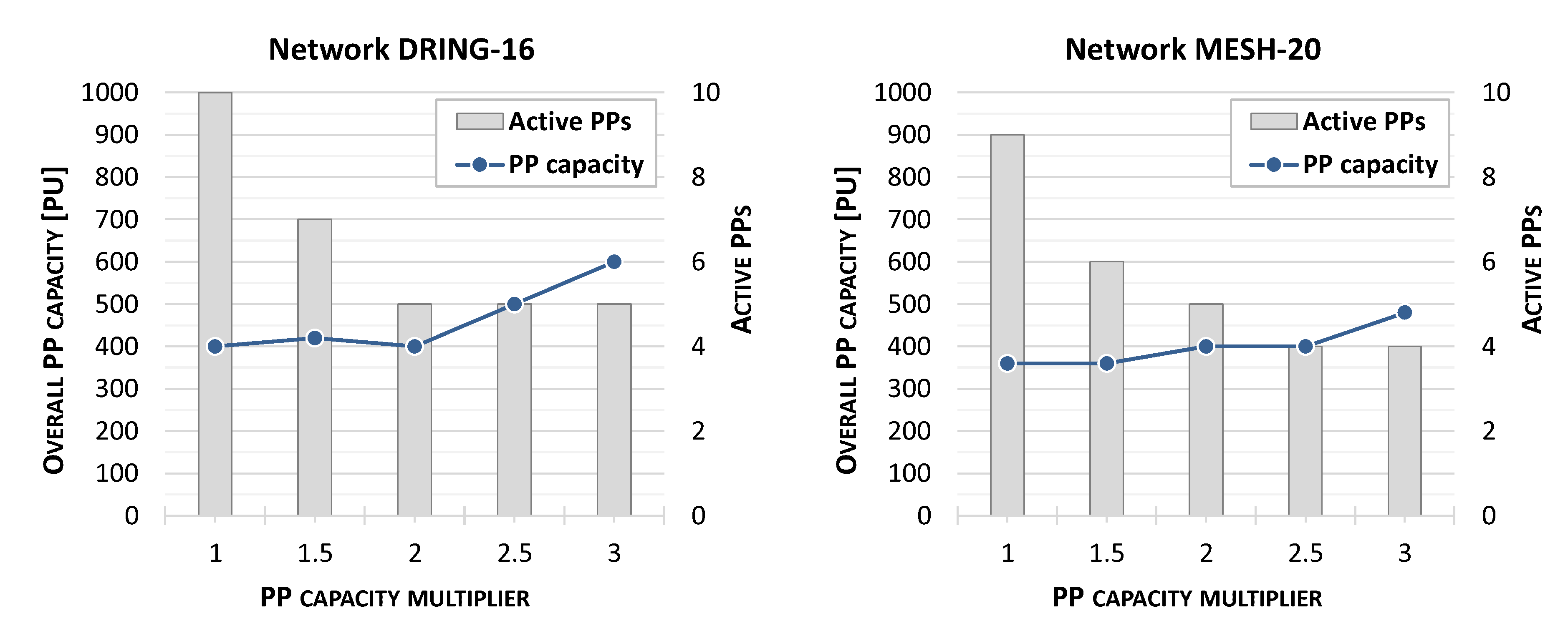
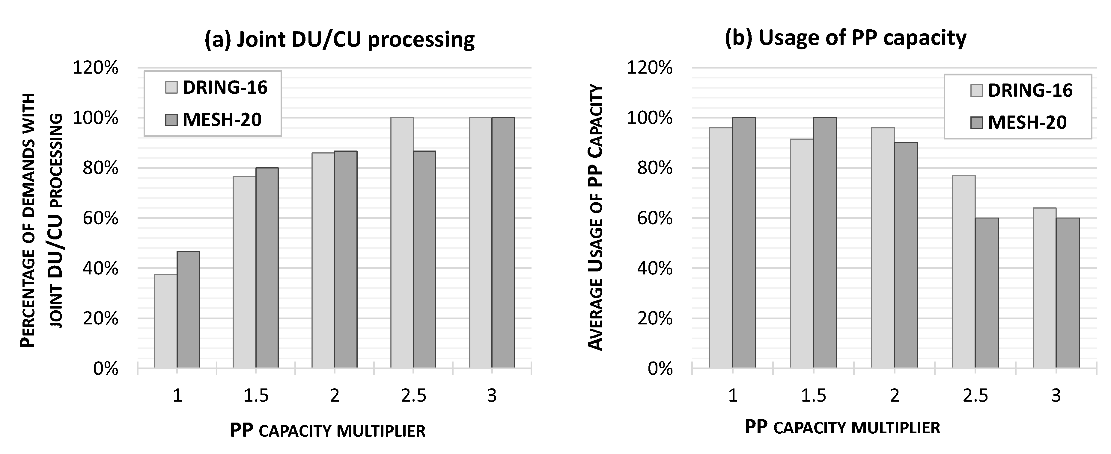
4.3. Evaluation of Larger Network Topologies
5. Conclusions
Funding
Conflicts of Interest
References
- Agiwal, M.; Roy, A.; Saxena, N. Next Generation 5G Wireless Networks: A Comprehensive Survey. IEEE Commun. Surv. Tutorials 2016, 18, 1617–1655. [Google Scholar] [CrossRef]
- The 3rd Generation Partnership Project (3GPP). Available online: http://www.3gpp.org/ (accessed on 28 September 2020).
- Peng, M.; Sun, Y.; Li, X.; Mao, Z.; Wang, C. Recent Advances in Cloud Radio Access Networks: System Architectures, Key Techniques, and Open Issues. IEEE Commun. Surv. Tutorials 2016, 18, 2282–2308. [Google Scholar] [CrossRef]
- Alimi, I.A.; Teixeira, A.; Monteiro, P. Towards an Efficient C-RAN Optical Fronthaul for the Future Networks: A Tutorial on Technologies, Requirements, Challenges, and Solutions. IEEE Commun. Surv. Tutor. 2018, 20, 708–769. [Google Scholar] [CrossRef]
- Gomes, N.J.; Sehier, P.; Thomas, H.; Chanclou, P.; Li, B.; Munch, D.; Jungnickel, V. Boosting 5G through Ethernet. IEEE Vehic. Technol. Mag. 2018, 55, 74–84. [Google Scholar] [CrossRef]
- ITU-T Technical Report; Transport Network Support of IMT-2020/5G; International Telecommunication Union: Geneva, Switzerland, 2018.
- IEEE. IEEE Standard for Packet-Based Fronthaul Transport Networks. Available online: https://standards.ieee.org/project/1914_1.html (accessed on 28 September 2020).
- IEEE. 802.1CM-2018—IEEE Standard for Local and Metropolitan Area Networks—Time-Sensitive Networking for Fronthaul; IEEE: Middlesex, NJ, USA, 2018. [Google Scholar]
- Garcia-Saavedra, A.; Salvat, J.X.; Li, X.; Costa-Perez, X. WizHaul: On the Centralization Degree of Cloud RAN Next Generation Fronthaul. IEEE Trans. Mob. Comput. 2018, 17, 2452–2466. [Google Scholar] [CrossRef]
- O-RAN Alliance. Available online: https://www.o-ran.org/ (accessed on 28 September 2020).
- IBM. CPLEX Optimizer. Available online: http://www.ibm.com/ (accessed on 28 September 2020).
- Carapellese, N.; Tornatore, M.; Pattavina, A.; Gosselin, S. BBU Placement over a WDM Aggregation Network Considering OTN and Overlay Fronthaul Transport. In Proceedings of the 2015 European Conference on Optical Communication (ECOC), Valencia, Spain, 27 September–1 October 2015. [Google Scholar]
- Musumeci, F.; Bellanzon, C.; Tornatore, N.C.M.; Pattavina, A.; Gosselin, S. Optimal BBU Placement for 5G C-RAN Deployment over WDM Aggregation Networks. IEEE J. Lightw. Technol. 2016, 34, 1963–1970. [Google Scholar] [CrossRef]
- Velasco, L.; Castro, A.; Asensio, A.; Ruiz, M.; Liu, G.; Qin, C.; Yoo, S.B. Meeting the Requirements to Deploy Cloud RAN Over Optical Networks. OSA/IEEE J. Opt. Commun. Netw. 2017, 9, B22–B32. [Google Scholar] [CrossRef]
- Wong, E.; Grigoreva, E.; Wosinska, L.; Machuca, C.M. Enhancing the Survivability and Power Savings of 5G Transport Networks based on DWDM Rings. OSA/IEEE J. Opt. Commun. Netw. 2017, 9, D74–D85. [Google Scholar] [CrossRef]
- Khorsandi, B.M.; Raffaelli, C. BBU location algorithms for survivable 5G C-RAN over WDM. Comput. Netw. 2018, 144, 53–63. [Google Scholar] [CrossRef]
- Liu, J.; Zhou, S.; Gong, J.; Niu, Z.; Xu, S. Graph-based Framework for Flexible Baseband Function Splitting and Placement in C-RAN. In Proceedings of the 2015 IEEE International Conference on Communications (ICC), London, UK, 8–12 June 2015. [Google Scholar]
- Koutsopoulos, I. Optimal Functional Split Selection and Scheduling Policies in 5G Radio Access Networks. In Proceedings of the 2017 IEEE International Conference on Communications Workshops (ICC Workshops), Paris, France, 21–25 May 2017. [Google Scholar]
- Ejaz, W.; Sharma, S.K.; Saadat, S.; Naeem, M.; Anpalagan, A.; Chughtai, N.A. A Comprehensive survey on Resource Allocation for CRAN in 5G and Beyond Networks. J. Net. Comput. Appl. 2020, 160, 1–24. [Google Scholar] [CrossRef]
- Wang, X.; Alabbasi, A.; Cavdar, C. Interplay of Energy and Bandwidth Consumption in CRAN with Optimal Function Split. In Proceedings of the 2017 IEEE International Conference on Communications (ICC), Paris, France, 21–25 May 2017. [Google Scholar]
- Alabbasi, A.; Wang, X.; Cavdar, C. Optimal Processing Allocation to Minimize Energy and Bandwidth Consumption in Hybrid CRAN. IEEE Trans. Green Commun. Netw. 2018, 2, 545–555. [Google Scholar] [CrossRef]
- Yu, H.; Musumeci, F.; Zhang, J.; Xiao, Y.; Tornatore, M.; Ji, Y. DU/CU Placement for C-RAN over Optical Metro-Aggregation Networks. In Proceedings of the 23rd Conference on Optical Network Design and Modelling, Athens, Greece, 13–16 May 2019. [Google Scholar]
- Xiao, Y.; Zhang, J.; Ji, Y. Can Fine-grained Functional Split Benefit to the Converged Optical-Wireless Access Networks in 5G and Beyond? IEEE Trans. Netw. Serv. Manag. 2020, 17, 1774–1787. [Google Scholar] [CrossRef]
- Nakayama, Y.; Hisano, D.; Kubo, T.; Fukada, Y.; Terada, J.; Otaka, A. Low-Latency Routing Scheme for a Fronthaul Bridged Network. OSA/IEEE J. Opt. Commun. Netw. 2018, 10, 14–23. [Google Scholar] [CrossRef]
- Hisano, D.; Nakayama, Y.; Kubo, T.; Uzawa, H.; Fukada, Y.; Terada, J. Decoupling of Uplink User and HARQ Response Signals to Relax the Latency Requirement for Bridged Fronthaul Networks. OSA/IEEE J. Opt. Commun. Netw. 2019, 11, B26–B36. [Google Scholar] [CrossRef]
- Klinkowski, M.; Mrozinski, D. Latency-Aware Flow Allocation in 5G NGFI Networks. In Proceedings of the 2020 22nd International Conference on Transparent Optical Networks (ICTON), Bari, Italy, 19–23 July 2020. [Google Scholar]
- Klinkowski, M. Optimization of Latency-Aware Flow Allocation in NGFI Networks. Comp. Commun. 2020, 161, 344–359. [Google Scholar] [CrossRef]
- 3GPP. Study on New Radio Access Technology: Radio Access Architecture and Interfaces; Technical Report 38.801, v14.0.0; European Telecommunications Standards Institute: Sophia Antipolis, France, 2017. [Google Scholar]
- Anritsu. 1914.3 (RoE) eCPRI Transport White Paper. 2018. Available online: https://dl.cdn-anritsu.com/en-en/test-measurement/files/Technical-Notes/White-Paper/mt1000a-ecpri-er1100.pdf (accessed on 28 September 2020).
- Imran, M.A.; Zaidi, S.A.R.; Shakir, M.Z. Access, Fronthaul and Backhaul Networks for 5G & Beyond; Institution of Engineering and Technology: London, UK, 2017. [Google Scholar]
- IEEE. 802.1CM-2018—IEEE Standard for Local and Metropolitan Area Networks—Bridges and Bridged Networks; IEEE: Middlesex, NJ, USA, 2018. [Google Scholar]
- Perez, G.O.; Larrabeiti, D.; Hernandez, J.A. 5G New Radio Fronthaul Network Design for eCPRI-IEEE 802.1CM and Extreme Latency Percentiles. IEEE Access 2019, 7, 82218–82229. [Google Scholar] [CrossRef]
- IEEE 1914 Working Group. Fronthaul Dimensioning Tool. Available online: https://sagroups.ieee.org/1914/p1914-1/ (accessed on 28 September 2020).
- Garey, M.R.; Johnson, D.R. Computers and Intractability: A Guide to the Theory of NPCompleteness; W H Freeman & Co: New York, NY, USA, 1979. [Google Scholar]
- Khorsandi, B.M.; Tonini, F.; Raffaelli, C. Centralized vs. Distributed Algorithms for Resilient 5G Access Networks. Phot. Netw. Commun. 2019, 37, 376–387. [Google Scholar] [CrossRef]
- Shehata, M.; Elbanna, A.; Musumeci, F.; Tornatore, M. Multiplexing Gain and Processing Savings of 5G Radio-Access-Network Functional Splits. IEEE Trans. Green Commun. Netw. 2018, 2, 982–991. [Google Scholar] [CrossRef]
- Klinkowski, M.; Walkowiak, K. An Efficient Optimization Framework for Solving RSSA Problems in Spectrally and Spatially Flexible Optical Networks. IEEE/ACM Trans. Netw. 2019, 27, 1474–1486. [Google Scholar] [CrossRef]


| Direction | Type of Flow | Flow Bit-Rate (Gbit/s) | Burst Size |
|---|---|---|---|
| Uplink | Fronthaul | 52 | |
| Midhaul | 6 | ||
| Backhaul | 6 | ||
| Downlink | Fronthaul | 60 | |
| Midhaul | 6 | ||
| Backhaul | 6 |
| Sets | |
|---|---|
| network nodes | |
| PP nodes; where | |
| network links | |
| switch output links | |
| demands | |
| uplink demands; | |
| downlink demands; | |
| types of flows; | |
| demand-flow pairs of an equal/higher priority than flow f of demand d | |
| demand-flow pairs of a lower priority than flow f of demand d | |
| allowable source nodes of flow f of demand d; | |
| allowable destination nodes of flow f of demand d; | |
| clusters of RUs | |
| Parameters | |
| if flow f of demand d originated in node i and terminated in node j is routed through link e | |
| cluster to which the RU of demand d belongs | |
| processing load of a DU | |
| processing load of a CU | |
| processing capacity of PP node | |
| bit-rate of flow f of demand d | |
| capacity (bit-rate) of link e | |
| propagation delay of link e | |
| store-and-forward delay produced in the origin node (switch) of link e | |
| delay produced by transmission of the burst of frames of flow f of demand d at link e | |
| maximum one-way latency of flow | |
| Variables | |
| binary, if flow f of demand d is realized between nodes i and j | |
| binary, if flow f of demand d is routed over link e | |
| binary, if flow f of demand d and flow of demand are routed over link e | |
| binary, if DU processing of demand d is performed in PP node v | |
| binary, if CU processing of demand d is performed in PP node v | |
| binary, if both CU and DU processing of demand d is performed in PP node v | |
| binary, if cluster c has assigned PP node v for DU processing | |
| binary, if PP node v is active | |
| continuous, latency of flow f belonging to demand d | |
| continuous, static latency in link e for flow f belonging to demand d | |
| continuous, dynamic latency in link e for flow f belonging to demand d | |
| continuous, latency in link e for flow f of demand d caused by higher/equal priority flows | |
| continuous, latency in link e for flow f of demand d caused by lower priority flows | |
| Network Link | Link Length (km) | Link Capacity (Gbit/s) |
|---|---|---|
| Switch–RU | 25 | |
| Switch–PP | 400 | |
| Switch–DC | 400 | |
| Switch–switch | 100 |
| Scenario | Optimization Results | |||||||
|---|---|---|---|---|---|---|---|---|
| Network | (s) | Active PPs | Latency [s] | |||||
| RING-10 | 80 | 1 | 715,485 | 715,668 | 0.03% | 10,800 | 7 | 15,668 |
| 2 | 418,224 | 418,224 | 0.00% | 935 | 4 | 18,224 | ||
| 3 | 418,224 | 418,224 | 0.00% | 446 | 4 | 18,224 | ||
| DRING-16 | 64 | 1 | 973,213 | 1,013,174 | 3.94% | 10,800 | 10 | 13,174 |
| 2 | 513,737 | 514,023 | 0.06% | 10,800 | 5 | 14,023 | ||
| 3 | 513,514 | 513,514 | 0.00% | 961 | 5 | 13,514 | ||
| 80 | 1 | 1,016,681 | 1,017,050 | 0.04% | 10,800 | 10 | 17,050 | |
| 2 | 521,205 | 521,443 | 0.05% | 10,800 | 5 | 21,443 | ||
| 3 | out-of-memory | |||||||
| MESH-20 | 40 | 1 | 805,959 | 805,959 | 0.00% | 696 | 8 | 5959 |
| 2 | 406,450 | 406,450 | 0.00% | 295 | 4 | 6450 | ||
| 3 | 405,822 | 405,822 | 0.00% | 91 | 4 | 5822 | ||
| 60 | 1 | 809,233 | 910,424 | 11.12% | 10,800 | 9 | 10,424 | |
| 2 | 463,297 | 510,047 | 9.17% | 10,800 | 5 | 10,047 | ||
| 3 | 412,050 | 412,050 | 0.00% | 348 | 4 | 12,050 | ||
Publisher’s Note: MDPI stays neutral with regard to jurisdictional claims in published maps and institutional affiliations. |
© 2020 by the author. Licensee MDPI, Basel, Switzerland. This article is an open access article distributed under the terms and conditions of the Creative Commons Attribution (CC BY) license (http://creativecommons.org/licenses/by/4.0/).
Share and Cite
Klinkowski, M. Latency-Aware DU/CU Placement in Convergent Packet-Based 5G Fronthaul Transport Networks. Appl. Sci. 2020, 10, 7429. https://doi.org/10.3390/app10217429
Klinkowski M. Latency-Aware DU/CU Placement in Convergent Packet-Based 5G Fronthaul Transport Networks. Applied Sciences. 2020; 10(21):7429. https://doi.org/10.3390/app10217429
Chicago/Turabian StyleKlinkowski, Mirosław. 2020. "Latency-Aware DU/CU Placement in Convergent Packet-Based 5G Fronthaul Transport Networks" Applied Sciences 10, no. 21: 7429. https://doi.org/10.3390/app10217429
APA StyleKlinkowski, M. (2020). Latency-Aware DU/CU Placement in Convergent Packet-Based 5G Fronthaul Transport Networks. Applied Sciences, 10(21), 7429. https://doi.org/10.3390/app10217429