Adaptive Command-Filtered Fuzzy Nonsingular Terminal Sliding Mode Backstepping Control for Linear Induction Motor

Abstract

This paper puts forward a projection-based adaptive command filtered fuzzy nonsingular terminal sliding mode backstepping (PACFTB) control method for the speed control of the linear induction motor (LIM) with unknown end effects. Firstly, the technique of fuzzy logic systems (FLS) is investigated to approximate the nonlinear components of the LIM’s mathematical model, which reduces the difficulty and cost of controller design. Then, a constrained command-filtered backstepping controller is designed with a filtering compensator compensating for the inherent error of constrained filter. Moreover, the nonsingular terminal sliding mode control method is combined in the controller design for its advantages of finite-time convergence of the system, and the projection-operator-based adaptive laws are established at the same time. Finally, the stability analysis proves that the boundedness and stability of all signals can be ensured with the proposed PACFTB controller, and the simulation results along with experiment results verify that the proposed control strategy has better control performance than the conventional command filter backstepping and PI controller.

1. Introduction

Linear induction motor (LIM) traction system has been widely applied in rail transit in recent years, due to its simple structure, low energy consumption, big start thrust and low cost [1,2,3]. The core component of the system is LIM and it is on focus for its extensive engineering application value and unique advantages like light weight, little noise, little pollution, good heat dissipation, strong climbing ability and so on [4,5]. However, in terms of LIM’s structure, it has a large magnetic circuit break and an initial gap, which makes its model more complicated than conventional induction motor. Related studies have shown that dynamic changes of system parameters, such as fluctuations in the air gap of linear motors, will lead to the first two levels of mutual inductance and LIM derivative resistance deviation [4,5], and the dynamic end effect makes the air gap magnetic field greatly affected by the inlet vortex in the high speed region of the motor [6]. These phenomena are serious at high speed, which increases the complexity of tracking and compensation control.

In recent years, a model reference adaptive indirect vector control method based on rotor time constant has been proposed and applied to LIM system with end effects to compensate for the bad influence brought by end effects in indirect vector control, achieving robust control of LIM speed [5,7,8]. To get better control performance, many nonlinear control methods are applied to LIMs, such as backstepping control [8,9], adaptive control [10,11,12], fuzzy control, neural network control [13,14,15] and sliding mode variable structure control [9,16,17]. Among them, backstepping is a useful tool for dealing with uncertain nonlinear systems. Backstepping is widely paid attention to with its distinct controller design principle and easy combination with modern control techniques to eliminate the influence of time-varying parameter and external disturbances on the system performance. Scholars have put forward many methods to solve the computational expansion problem such as dynamic surface control [18,19] and constrained command filter [8,20,21]. In [8], the adaptive backstepping control method is studied with fuzzy logic technique for LIM. However, it lacks measures to ensure the robustness and dynamic performance when facing end effects in LIM. In [18], a disturbance-observer based fast terminal sliding mode backstepping control is proposed for uncertain nonlinear systems, where the first-order filter is introduced to solve the computational expansion problem in the high-order backstepping control system. However, the design process and structure of the disturbance observer is complex, which increases the cost of computation and difficulty of controller design for LIM with end effects. Besides, the influence of the filtering error of the first-order filter on the system is not considered. Hence, more work shall be implemented against these problems on the control of LIM.

Fuzzy logic system (FLS) has been widely concerned by researchers for its universal approximation property and ingenious treatment of nonlinear terms, which makes the controller design process simple and distinct [11,22,23]. Besides, the sliding mode control (SMC) method has low accuracy and strong robustness to the model, which has a good control effect on parameter perturbation and external disturbance [24,25]. Among several SMC methods, the nonsingular terminal SMC has distinct advantages in finite convergence time [26,27]. It guarantees the robustness, dynamic and static performance of the system. Comparing common terminal SMC, it can eliminate the singularity of terminal SMC and achieve better performance [28,29]. When the system state gets far from the origin, the convergence time will be still limited under nonsingular terminal SMC and the dynamic characteristics of the system would be better [30,31]. Therefore, the fuzzy logic technique and nonsingular terminal SMC method can be both integrated in the investigated adaptive backstepping control strategy for better control performance of LIM.

Motivated by the above investigation on control methods of LIM, a projection-based adaptive command filtered fuzzy nonsingular terminal sliding mode backstepping (PACFTB) control strategy is proposed for better speed control performance of LIM. The controlled plant is the LIM with unknown end effects and the control objective is to make the speed tracking have high precision and quick response against variable trajectory. The main contributions of this paper are given as follows.

• The nonsingular terminal sliding mode control method is integrated with the adaptive fuzzy backstepping control to enhance the robustness of the system and ensure to reach the equilibrium point within a limited time.
• The fuzzy logic technique is introduced to estimate the nonlinear part of the system model to make the controller design process more clear and easy, and the stability proof of the proposed PACFTB control strategy is provided concretely.
• The simulations and experiments are both carried out and discussed to further prove the effectiveness of the proposed PACFTB control strategy.

The structure of the article is arranged as follows. Section 2 describes the mathematical model of LIM with unknown end effects and introduces the FLS and projection operators. In Section 3, an FLS-based adaptive command-filtered backstepping control strategy combining nonsingular terminal SMC is developed for LIM while detailed design process is given step by step, and the stability analysis is given in Section 4. Section 5 provides the simulation and experimental results and discussions to verify the progressiveness of the proposed control strategy. Finally, we summarize the whole paper and draw conclusions in Section 6.

2. Establishment of LIM Dynamic Model and Preliminaries

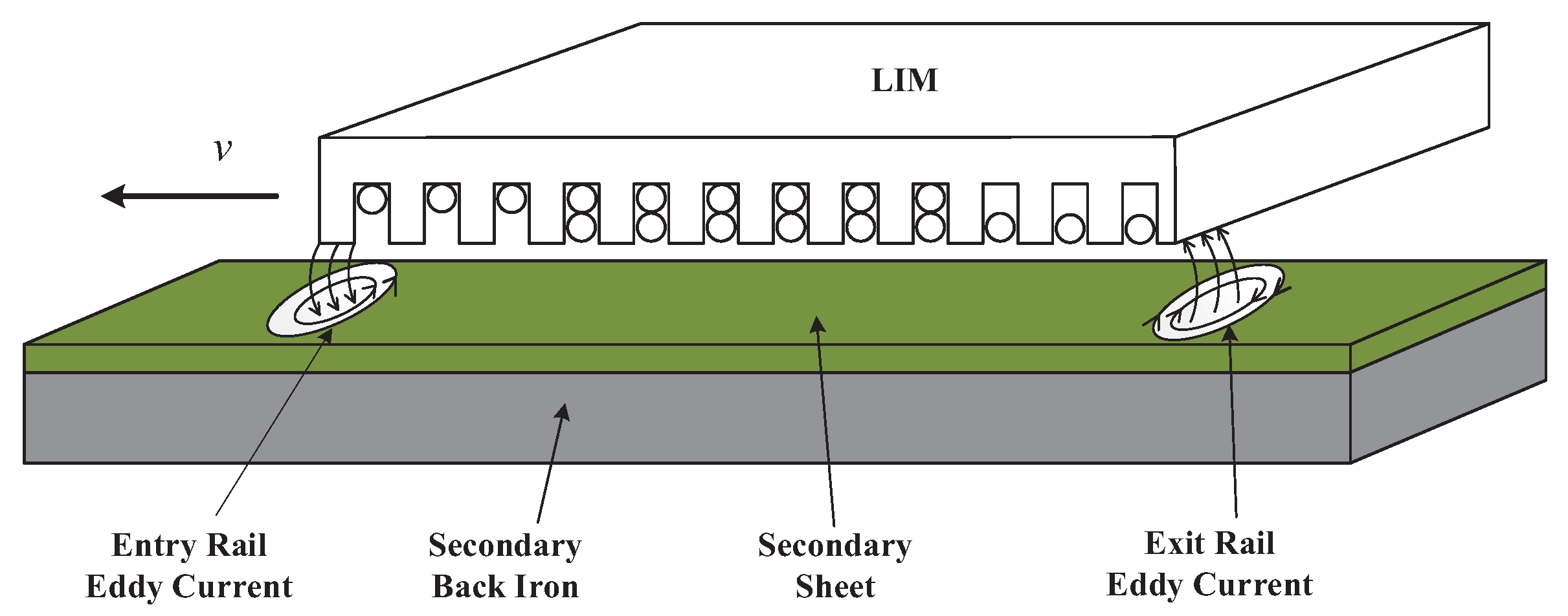
2.1. Establishment of LIM Dynamic Model

The sketch map of LIM can be seen in Figure 1. LIM is like a rotary induction motor (RIM) that is tiled. The difference between LIM and RIM lies in the existence of end effect in LIM, and the dimensionless coefficient Q represent the magnitude of end effect, it can be derived from the speed of LIM calculated as [5,7,8]:

$$\begin{array}{c}\hfill Q=\frac{l·R_r}{L_r·v}\end{array}$$

(1)

where l means the primary length; $R_r$, $L_r$ represent secondary resistance and inductance, respectively; v denotes the speed.

In this paper, the main goal is to control LIMs like DC motors, while ensuring superior performance. According to [7,10], the equivalent circuit and flux linkage in $dq-axis$ are expressed as follows.

$$\begin{array}{c}\hfill \begin{array}{c}{U}_{ds}=R_s{i}_{ds}+p{\psi }_{ds}-{\omega }_e{\psi }_{sq}\hfill \\ U_{qs}=R_s{i}_{qs}+p{\psi }_{qs}-{\omega }_e{\psi }_{sd}\hfill \\ U_{dr}=R_r{i}_{dr}+p{\psi }_{dr}-\left({\omega }_e-{\omega }_r\right){\psi }_{rq}\hfill \\ U_{qr}=R_r{i}_{qr}+p{\psi }_{qr}+\left({\omega }_e-{\omega }_r\right){\psi }_{rd}\hfill \end{array}\end{array}$$

(2)

$$\begin{array}{c}\hfill \begin{array}{c}{\psi }_{ds}=L_{sl}{i}_{ds}+L_m(1-f\left(Q\right))(i_{ds}+i_{dr})\hfill \\ {\psi }_{qs}=L_{sl}{i}_{qs}+L_m(1-f\left(Q\right))(i_{qs}+i_{qr})\hfill \\ {\psi }_{dr}=L_{rl}{i}_{dr}+L_m(1-f\left(Q\right))(i_{ds}+i_{dr})\hfill \\ {\psi }_{qr}=L_{rl}{i}_{qr}+L_m(1-f\left(Q\right))(i_{qs}+i_{qr})\hfill \end{array}\end{array}$$

(3)

where $f\left(Q\right)=(1-e^{-Q})/Q$; $U_{ds}$, $U_{qs}$, $i_{ds}$, $i_{qs}$, ${\psi }_{ds}$, ${\psi }_{qs}$ denote the primary voltage, current and flux linkage in $d-q$ axis, and $U_{dr}$, $U_{qr}$, $i_{dr}$, $i_{qr}$, ${\psi }_{dr}$, ${\psi }_{qr}$ denote the secondary voltage, current and flux linkage in $d-q$ axis, respectively. Notice that the d-q axis is relative to the rotor. For the motor, the d-axis is the axis where the magnetic pole of the rotor is located while the q-axis is perpendicular to the d-axis and rotates 90 degrees along the d-axis anticlockwise. Besides, $R_s$ is the primary resistance; ${\omega }_e$ and ${\omega }_r$ are the synchronous speed and secondary speed; p is the differential operator; $L_{sl}$ and $L_{rl}$ are the primary and secondary leakage inductance.

By virtue of the indirect vector control (IVC) technique, the linear induction motor model is transformed into a DC motor model, which is shown as follows [8,24].

$$\begin{array}{c}\hfill \begin{array}{c}{\psi }_{qr}={\dot{\psi }}_{qr}=0\hfill \\ U_{dr}=U_{qr}=0\hfill \end{array}\end{array}$$

(4)

Then the LIM mathematical model can be described as [7,10]

$${\dot{i}}_{ds}=-\frac{R_s}{L\left(Q\right)}{i}_{ds}+\frac{U_{ds}}{L\left(Q\right)}+{\omega }_e{i}_{qs}$$

(5)

$$\begin{array}{cc}\hfill {\dot{i}}_{qs}=& -{\omega }_e\left[i_{ds}+\frac{L_m\left(1-f\left(Q\right)\right)}{L\left(Q\right)\left(L_r-L_{m}f\left(Q\right)\right)}{\psi }_{dr}\right]\hfill \\ & -\frac{R_s}{L\left(Q\right)}{i}_{qs}+\frac{U_{qs}}{L\left(Q\right)}\hfill \end{array}$$

(6)

$$\begin{array}{cc}\hfill {\psi }_{dr}& =\frac{L_m\left[1-f\left(Q\right)\right]}{1+\left[T_r-L_{m}f\left(Q\right)/R_r\right]p}{i}_{ds}\hfill \end{array}$$

(7)

$$\begin{array}{cc}\hfill {\omega }_{sl}& ={\omega }_e-{\omega }_r=\frac{L_m\left[1-f\left(Q\right)\right]}{T_r-L_{m}f\left(Q\right)/R_r}\frac{i_{qs}}{{\psi }_{dr}}\hfill \end{array}$$

(8)

$$\begin{array}{cc}\hfill F_e& =K_T{i}_{qs}=M·\dot{v}+D·v+F_L\hfill \end{array}$$

(9)

where $T_r=L_r/R_r$; $K_T=\frac{3}{2}P\frac{\pi }{h}\frac{L_m\left(1-f\left(Q\right)\right)}{L_r-L_{m}f\left(Q\right)}{\psi }_{dr}$; $L\left(Q\right)=L_s-L_{m}f\left(Q\right)-\frac{{\left[L_m\left(1-f\left(Q\right)\right)\right]}^2}{L_r-L_{m}f\left(Q\right)}$; ${\omega }_{sl}$ denotes the slip frequency; D denotes the viscous friction coefficient; M denotes the total mass of mover; P denotes the number of pole pairs and h denotes the number of pole pitch; $F_L$ denotes the external force disturbance.

According to (9), we can get the accelerated velocity of LIM as:

$$\dot{v}=\frac{K_T}{M}{i}_{qs}+\Phi v+F$$

(10)

where $\Phi =-D/M$, $F=-F_L/M$.

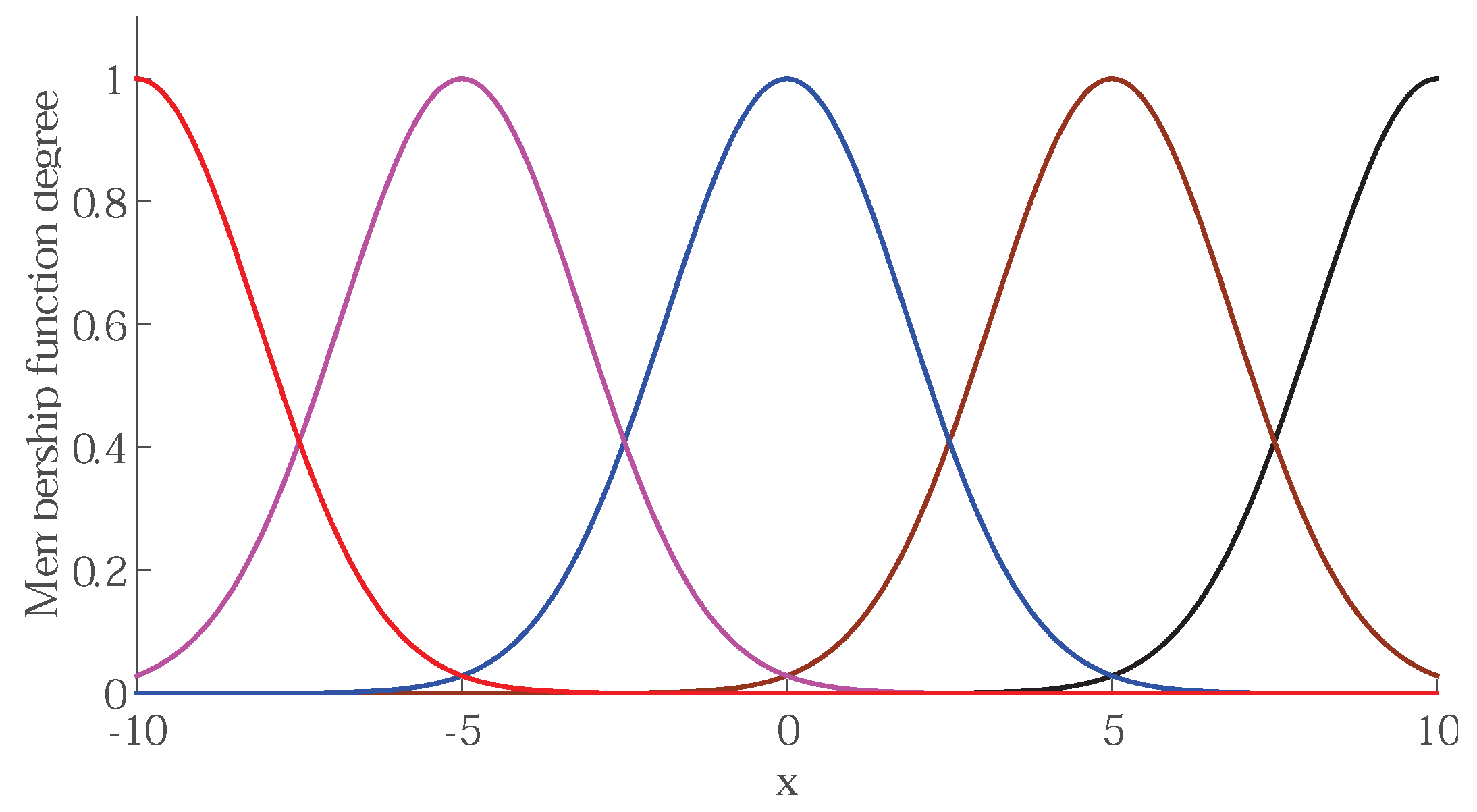
2.2. Fuzzy Logic System (FLS)

In fact, all the parameters of the system cannot be correctly estimated because of many reasons. Firstly, when measuring the values of resistance, inductance and capacitance, we cannot guarantee the accuracy of the measuring tool. Secondly, when the LIM works, the temperature and other environmental factors in the system will cause the parameters to change greatly or slightly. Thus, so as to weaken or even eliminate the effects of uncertain nonlinear functions and parameters on speed control, FLS is applied whose fuzzy rules are deduced as [11]:

$$\mathrm{IF}{x}_1\mathrm{is}{F}_1^j\mathrm{and}\cdots \mathrm{and}{x}_n\mathrm{is}{F}_n^j\mathrm{Then}y\mathrm{is}{A}^j$$

where $j=1,2,\cdots ,N$; $x={\left[x_1,x_2,\cdots ,x_n\right]}^T\in R^n$ is the input FLS while $y\in R$ is the output; $F_i^j$ and $A^j$ are the fuzzy sets. Thus, we can get the output of the FLS as:

$$y\left(x\right)=\frac{{\displaystyle \sum _{j=1}^N}{w}_j{\displaystyle \prod _{i=1}^n}{\mu }_i^j\left(x_i\right)}{{\displaystyle \sum _{j=1}^N}{\displaystyle \prod _{i=1}^n}{\mu }_i^j\left(x_i\right)}$$

(11)

where $w_j$ is defined as the parameter of the consequent part $A^j$, ${\mu }_i^j\left(x_i\right)$ the fuzzy membership function. Let $b_j\left(x\right)=\frac{{\displaystyle \prod _{i=1}^n}{\mu }_i^j\left(x_i\right)}{{\displaystyle \sum _{j=1}^N}{\displaystyle \prod _{i=1}^n}{\mu }_i^j\left(x_i\right)}$, $B\left(x\right)={[b_1\left(x\right),b_2\left(x\right),\cdots ,b_N\left(x\right)]}^T$ is fuzzy basis function vector, so the FLS could be overwritten as:

$$y\left(x\right)=W^{T}B\left(x\right)$$

(12)

The following lemma can be guaranteed once all the fuzzy membership functions belong to Gussian functions:

Lemma 1.

[11]: If function $g\left(x\right)$ is on a compact set Λ, then the FLS gets the following property for any $\varsigma >0$:

$$\underset{y\in \Lambda }{sup}\left|g\left(x\right)-y\left(x\right)\right|\le \varsigma$$

(13)

2.3. Projection Operator

In this subsection, we introduce projection operators to ensure boundedness of adaptive estimates [12].

Here we use $\widehat{\phi }$ and $\tilde{\phi }$ to represent the estimated value and estimation error of $\phi$, then the projection opertaor adaptive law can be written as:

$$\widehat{\phi }=\mathrm{Pro}{\mathrm{j}}_{\widehat{\phi }}\left(\tau \varphi \right)$$

(14)

where $\varphi$ represents the designed traditional adaptive law and $\tau$ represents a positive constant. Referring to [22], the projection mapping $\mathrm{Pro}{\mathrm{j}}_{\widehat{\phi }}\left(\tau \varphi \right)={\left[\mathrm{Pro}{\mathrm{j}}_{{\widehat{\phi }}_1}\left(\tau {\varphi }_1\right),\cdots ,\mathrm{Pro}{\mathrm{j}}_{{\widehat{\phi }}_k}\left(\tau {\varphi }_k\right)\right]}^T$ is defined as:

$$\begin{array}{c}\hfill \mathrm{Pro}{\mathrm{j}}_{{\widehat{\phi }}_i}\left(\tau {\varphi }_i\right)=\left\{\begin{array}{c}0,\mathrm{if}{\widehat{\phi }}_i={\phi }_{imax}\mathrm{and}\tau {\varphi }_i>0\hfill \\ 0,\mathrm{if}{\widehat{\phi }}_i={\phi }_{imin}\mathrm{and}\tau {\varphi }_i<0\hfill \\ {\varphi }_i,\mathrm{otherwise}\hfill \end{array}\right.\end{array}$$

(15)

As for each adaptive function $\varphi$, the defined projection operation has the properties described as [16]:

Property 1.

$\widehat{\phi }\in {\Omega }_{\theta }\stackrel{\Delta }{=}\left\{\widehat{\phi }:{\phi }_{min}\le \widehat{\phi }\le {\phi }_{max}\right\}$

Property 2.

${\tilde{\phi }}^T\left[\mathrm{Pro}{\mathrm{j}}_{\widehat{\phi }}\left(\tau \varphi \right)-\tau \varphi \right]\le 0,\forall \varphi$

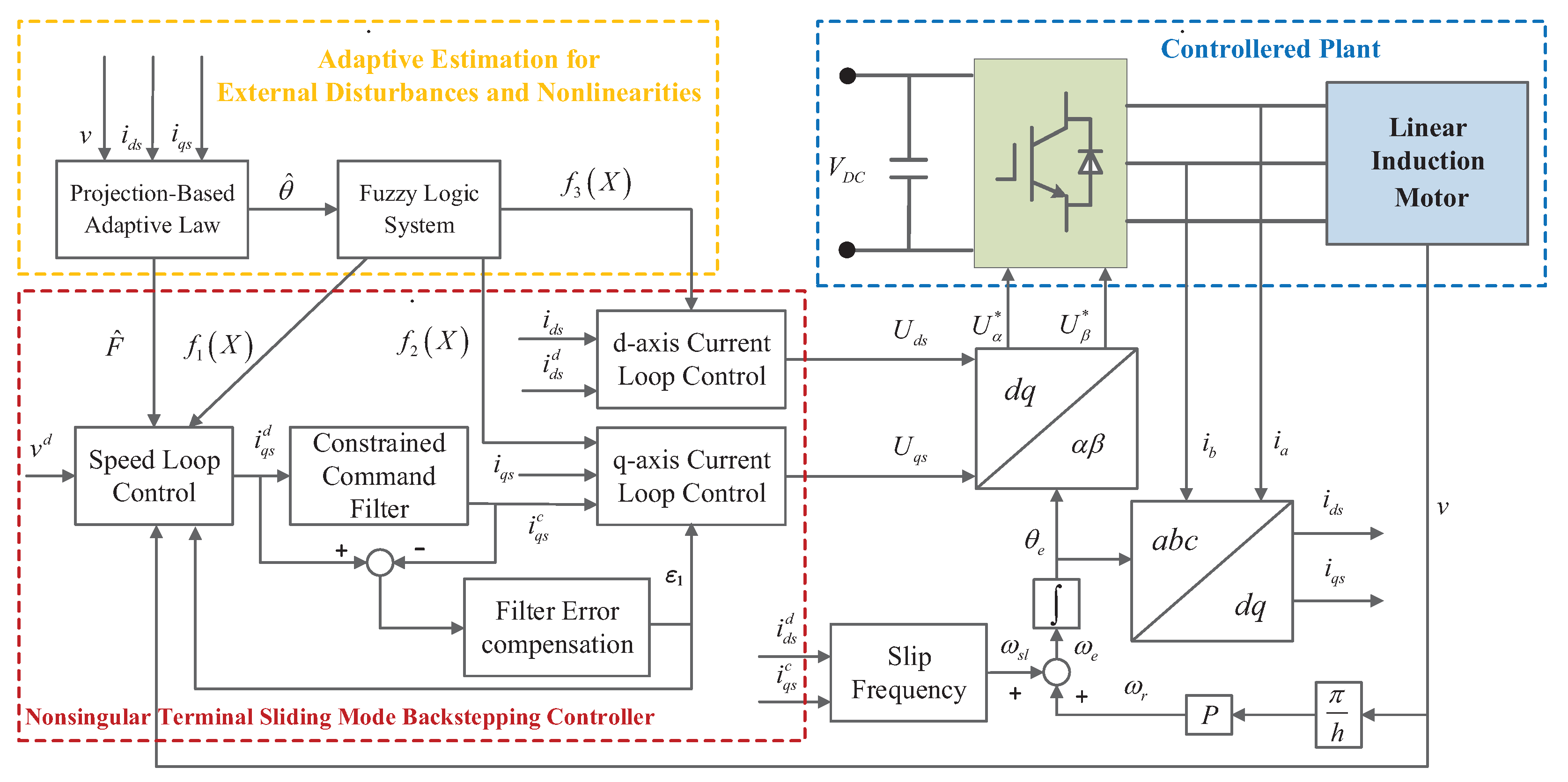
3. Design Process of the PACFTB Controller

So as to ensure the following effect of LIM speed, a PACFTB method is designed. First, corresponding to the backstepping method, the tracking errors could be written as:

$$e_1=v-v^d$$

(16)

$$e_2=i_{qs}-i_{qs}^c$$

(17)

$$e_3=i_{ds}-i_{ds}^d$$

(18)

where $v^d$ and $i_{ds}^d$ are given velocity reference and d-axis primary current, $i_{qs}^c$ the given reference from constrained command filter based on speed loop control. The command filter can reduce the differential expansion problem in backstepping control and reduce the computational complexity of the controller. Then, the mathematical form of command filter can be written as [8]:

$$\begin{array}{c}\hfill \left[\begin{array}{c}{\dot{z}}_1\hfill \\ {\dot{z}}_2\hfill \end{array}\right]=\left[\begin{array}{c}{z}_2\\ 2\xi {\omega }_n\left[S_R\left(\frac{{\omega }_n^2}{2\xi {\omega }_n}\left(S_M\left(u\right)-z_1\right)\right)-z_2\right]\end{array}\right]\end{array}$$

(19)

where $u=x^d$; $\xi$ denotes the dampling of the system while ${\omega }_n$ denotes the bandwidth; $S_M(·)$ and $S_R(·)$ represent the magnitude and rate boundedness, respectively. Through the application of command filters, differential signal ${\dot{x}}^c$ could be obtained by integration, and this would eliminate the magnified interference problems caused by practical applications.

Whereas, due to the use of command filters, there will be filtering error $\mu =x^c-x^d$ which can interfere with the following performance and that must be taken into consideration. An effective method is by properly increasing ${\omega }_n$, the output $x^c$ can quickly coverage to $x^d$, and the filtering error can be reduced. Furthermore, this paper uses a filter compensator signal to eliminate the filter error as follows:

$${\dot{\epsilon }}_1=-k_1{\epsilon }_1+\left(i_{qs}^c-i_{qs}^d\right)$$

(20)

where $k_1>0$ is a positive constant, ${\epsilon }_1$ is the compensation signal of the filter.

Then, a redefined tracking error signal ${\overline{e}}_1$ is given as:

$${\overline{e}}_1=e_1-{\epsilon }_1$$

(21)

Define the nonsingular terminal sliding surface as follows:

$$S_d=e_3+k_d{\left({\int }_0^t{e}_{3}dt\right)}^{p_1/q_1}=e_3+k_d{I_d}^{p_1/q_1}$$

(22)

$$S_q=e_2+k_q{\left({\int }_0^t{e}_{2}dt\right)}^{p_2/q_2}=e_2+k_q{I_q}^{p_2/q_2}$$

(23)

where $I_d={\int }_0^t{e}_{3}dt$, $I_q={\int }_0^t{e}_{2}dt$, $k_d,k_q>0$ are the designed constant of the nonsingular terminal sliding surface, $p_1,p_2,q_1,q_2$ are the positive odd numbers and $1<p_1/q_1<2$, $1<p_2/q_2<2$.

Suppose that at $t_r$, $S_d$ converges to zero, then, according to (22), ${\int }_0^t{e}_{3}dt$ and $e_3$ converges to zero within a limited time which is [32]:

$$t_s=\frac{q_1}{k_d\left(p_1-q_1\right)}{I}_d{\left(t_r\right)}^{\frac{q_1}{p_1-q_1}}$$

(24)

where $I_d\left(t_r\right)=-{\left[k_d^{-1}{e}_2\left(t_r\right)\right]}^{q_1/p_1}$, thus, it is concluded that terminal sliding surface can make the controlled system converge from any state to origin point in finite time $t_s+t_r$. Similarly, the convergence time can be calculated when the system reaches the equilibrium point along with terminal sliding surface $S_q$.

Step 1: So as to get the virtual control formula for $i_{qs}^d$, the following Lyapunov function is designed:

$$V_1=\frac{1}{2}{\overline{e}}_1^2$$

(25)

Then, it is further calculated as:

$$\begin{array}{cc}\hfill {\dot{V}}_1& ={\overline{e}}_1\left(\frac{K_T}{M}{i}_{qs}+\Phi v+F-{\dot{v}}^d+k_1{\epsilon }_1-i_{qs}^c+i_{qs}^d\right)\hfill \\ \hfill & ={\overline{e}}_1\left(i_{qs}-{\dot{v}}^d+k_1{\epsilon }_1-i_{qs}^c+i_{qs}^d+f_1\left(X\right)+F\right)\hfill \\ \hfill & =-k_1{\overline{e}}_1^2+{\overline{e}}_1\left(e_2-{\dot{v}}^d+i_{qs}^d+f_1\left(X\right)+F+k_1{e}_1\right)\hfill \end{array}$$

(26)

where $f_1\left(X\right)=\frac{K_T}{M}{i}_{qs}+\Phi v-i_{qs}$, and $X={\left[v,i_{qs}\right]}^T$ is defined the input of the FLS. According to the Lemma 1, we have the following FLS:

$$f_1\left(X\right)=W_1^T{B}_1\left(X\right)+{\xi }_1\left(X\right)$$

(27)

where ${\xi }_1\left(X\right)$ denotes the approximation error and satisfies the condition $‖{\xi }_1\left(X\right)‖\le {\varsigma }_1$. Referring to (32) and Young’s inequality, the following inequality can be obtained:

$$\begin{array}{cc}\hfill {\overline{e}}_1{f}_1\left(X\right)& ={\overline{e}}_1{W}_1^T{B}_1\left(X\right)+{\overline{e}}_1{\xi }_1\left(X\right)\hfill \\ \hfill & \le {\overline{e}}_1{W}_1^T{B}_1\left(X\right)+\frac{1}{2}{\overline{e}}_1^2+\frac{1}{2}{\varsigma }_1^2\hfill \end{array}$$

(28)

Then, the ${\dot{V}}_1$ has the following unequal relation:

$$\begin{array}{cc}\hfill {\dot{V}}_1& \le -k_1{\overline{e}}_1^2+\frac{1}{2}{\varsigma }_1^2+{\overline{e}}_1\left(e_2-{\dot{v}}^d+i_{qs}^d+W_1^T{B}_1\left(X\right)+F+k_1{e}_1+\frac{1}{2}{\overline{e}}_1\right)\hfill \end{array}$$

(29)

Therefore, the virtual controller $i_{qs}^d$ can be chosen as:

$$i_{qs}^d={\dot{v}}^d-{{\widehat{W}}_1}^T{B}_1\left(X\right)-k_1{e}_1-\frac{1}{2}{\overline{e}}_1-\widehat{F}-e_2$$

(30)

where $\widehat{F}$ means the estimation value of F that is used to deal with the problem caused by load disturbance, ${\widehat{W}}_1$ the estimation value of weight vector $W_1$, then the following inequations can be obtained as:

$${\dot{V}}_1\le -k_1{\overline{e}}_1^2+\frac{1}{2}{\varsigma }_1^2+{\overline{e}}_1{\left(W_1-{\widehat{W}}_1\right)}^T{B}_1\left(X\right)-{\overline{e}}_1\tilde{F}$$

(31)

where $\tilde{F}=\widehat{F}-F$ denotes the adaptive estimation error.

Step 2: In order to obtain the control law in $q-axis$, the Lyapunov function $V_2$ is selected as:

$$V_2=V_1+\frac{1}{2}{S}_q^2$$

(32)

Then the derivative of $V_2$ can be figured by:

$${\dot{V}}_2={\dot{V}}_1+S_q{\dot{S}}_q$$

(33)

From (6) and (23), $S_q{\dot{S}}_q$ is calculated as:

$$\begin{array}{cc}\hfill S_q{\dot{S}}_q& =S_q\left(-{\omega }_e\left[i_{ds}+\frac{L_m\left(1-f\left(Q\right)\right)}{L\left(Q\right)\left(L_r-L_{m}f\left(Q\right)\right)}{\psi }_{dr}\right]-\frac{R_s}{L\left(Q\right)}{i}_{qs}+\frac{U_{qs}}{L\left(Q\right)}-{\dot{i}}_{qs}^c+{k_q}^{p_2/q_2}{e}_2{I}_q^{p_2/q_2-1}\right)\hfill \\ \hfill & =S_q\left(f_2\left(X\right)+U_{qs}-{\dot{i}}_{qs}^c+{k_q}^{p_2/q_2}{e}_2{I}_q^{p_2/q_2-1}\right)\hfill \end{array}$$

(34)

where

$$\begin{array}{cc}\hfill f_2\left(X\right)& =-{\omega }_e\left[i_{ds}+\frac{L_m\left(1-f\left(Q\right)\right)}{L\left(Q\right)\left(L_r-L_{m}f\left(Q\right)\right)}{\psi }_{dr}\right]-\frac{R_s}{L\left(Q\right)}{i}_{qs}+\frac{U_{qs}}{L\left(Q\right)}-U_{qs}\hfill \\ \hfill & =W_2^T{B}_2\left(X\right)+{\xi }_2\left(X\right)\hfill \end{array}$$

(35)

with $‖{\xi }_2\left(X\right)‖\le {\varsigma }_2$. $X={\left[i_{ds},i_{qs}\right]}^T$ is defined the input of the FLS. Similarly, for given ${\varsigma }_2>0$, the following inequality can be confirmed:

$$S_q{f}_2\left(X\right)\le S_q{W}_2^T{B}_2\left(X\right)+\frac{1}{2}{S}_q^2+\frac{1}{2}{\varsigma }_2^2$$

(36)

Substituting (34) and (36) into (33), then gets

$$\begin{array}{cc}\hfill {\dot{V}}_2& \le -k_1{\overline{e}}_1^2+\frac{1}{2}{\varsigma }_1^2+\frac{1}{2}{\varsigma }_2^2+{\overline{e}}_1{\left(W_1-{\widehat{W}}_1\right)}^T{B}_1\left(X\right)-{\overline{e}}_1\tilde{F}\hfill \\ \hfill & +S_q\left(W_2^T{B}_2\left(X\right)+U_{qs}-{\dot{i}}_{qs}^c+\frac{1}{2}{S}_q+{k_q}^{p_2/q_2}{e}_2{I}_q^{p_2/q_2-1}\right)\hfill \end{array}$$

(37)

To meet the conditions $S_q{\dot{S}}_q<0$, the exponential convergence law is adopted as the following:

$${\dot{S}}_q=-k_2{S}_q-k_q\mathrm{sign}\left(S_q\right)$$

(38)

where $k_2>0$ and $k_q>0$ are the designed positive constant, function $\mathrm{sign}\left(·\right)$ represents the symbolic function which defined as:

$$\mathrm{sign}\left(·\right)=\left\{\begin{array}{cc}\overline{x}/\left|\overline{x}\right|,\hfill & \mathrm{if}\overline{x}\ne 0\\ 0,\hfill & \mathrm{if}\overline{x}=0\end{array}\right.$$

(39)

Then, the controller $U_{qs}$ can be chosen as:

$$\begin{array}{c}\hfill U_{qs}=-{{\widehat{W}}_2}^T{B}_2\left(X\right)+{\dot{i}}_{qs}^c-\frac{1}{2}{S}_q-k_2{S}_q-k_q\mathrm{sign}\left(S_q\right)-{k_q}^{p_2/q_2}{e}_2{I}_q^{p_2/q_2-1}\end{array}$$

(40)

Afterwards, the derivative of $V_2$ can be calculated as:

$$\begin{array}{cc}\hfill {\dot{V}}_2& \le -k_1{\overline{e}}_1^2-k_2{S}_q^2-k_q\left|S_q\right|+\frac{1}{2}{\varsigma }_1^2+\frac{1}{2}{\varsigma }_2^2-{\overline{e}}_1\tilde{F}+{\overline{e}}_1{\left(W_1-{\widehat{W}}_1\right)}^T{B}_1\left(X\right)\hfill \\ \hfill & +S_q{\left(W_2-{\stackrel{}{W}}_2\right)}^T{B}_2\left(X\right)\hfill \end{array}$$

(41)

Step 3: In order to design the control law of d-axis, the Lyapunov function $V_3$ is chosen as:

$$V_3=V_2+\frac{1}{2}{S}_d^2$$

(42)

Then we can get the derivative of $V_3$ as:

$$\begin{array}{cc}\hfill {\dot{V}}_3& ={\dot{V}}_2+S_d\left(-\frac{R_s}{L\left(Q\right)}{i}_{ds}+\frac{U_{ds}}{L\left(Q\right)}+{\omega }_e{i}_{qs}-{\dot{i}}_{ds}^d+{k_d}^{p_1/q_1}{e}_3{I}_d^{p_1/q_1-1}\right)\hfill \\ \hfill & ={\dot{V}}_2+S_d\left(U_{ds}+f_3\left(X\right)-{\dot{i}}_{ds}^d+{k_d}^{p_1/q_1}{e}_3{I}_d^{p_1/q_1-1}\right)\hfill \end{array}$$

(43)

where

$$\begin{array}{cc}\hfill f_3\left(X\right)& =-\frac{R_s}{L\left(Q\right)}{i}_{ds}+\frac{U_{ds}}{L\left(Q\right)}+{\omega }_e{i}_{qs}-U_{ds}\hfill \\ \hfill & =W_3^T{B}_3\left(X\right)+{\xi }_3\left(X\right)\hfill \end{array}$$

(44)

with $‖{\xi }_3\left(X\right)‖\le {\varsigma }_3$. $X={\left[i_{ds},i_{qs}\right]}^T$ is defined as the input of the FLS. Similarly to the front, through Lemma 1, (46) and Young’s inequality, the following inequality can be obtained:

$$\begin{array}{c}\hfill S_d{f}_3\left(X\right)\le S_d{W}_3^T{B}_3\left(X\right)+\frac{1}{2}{S}_d^2+\frac{1}{2}{\varsigma }_3^2\end{array}$$

(45)

where ${\varsigma }_3>0$ is any given constant.

Substituting (45) into (43), one obtain:

$$\begin{array}{cc}\hfill {\dot{V}}_3\le & {\dot{V}}_2+\frac{1}{2}{\varsigma }_3^2+S_d(U_{ds}+W_3^T{B}_3\left(X\right).\hfill \\ \hfill & \left.+\frac{1}{2}{S}_d-{\dot{i}}_{ds}^d+{k_d}^{p_1/q_1}{e}_3{I}_d^{p_1/q_1-1}\right)\hfill \end{array}$$

(46)

Similarly, the exponential convergence law is adopted as follows:

$${\dot{S}}_d=-k_3{S}_d-k_d\mathrm{sign}\left(S_d\right)$$

(47)

where $k_3>0$ and $k_d>0$ are the designed positive constant.

Then, the real controller for $U_{ds}$ can be chosen as:

$$\begin{array}{c}\hfill U_{ds}=-{{\widehat{W}}_3}^T{B}_3\left(X\right)-\frac{1}{2}{S}_d+{\dot{i}}_{ds}^d-k_3{S}_d-k_d\mathrm{sign}\left(S_d\right)-{k_d}^{p_1/q_1}{e}_3{I}_d^{p_1/q_1-1}\end{array}$$

(48)

Thus, we can reach ${\dot{V}}_3$ as

$$\begin{array}{cc}\hfill {\dot{V}}_3\le & -k_1{\overline{e}}_1^2-k_2{S}_q^2-k_3{S}_d^2-{\overline{e}}_1\tilde{F}-k_d\left|S_d\right|-k_q\left|S_q\right|+\frac{1}{2}\sum _{i=1}^3{\varsigma }_i^2-{\overline{e}}_1{{\tilde{W}}_1}^T{B}_1\left(X\right)\hfill \\ \hfill & S_q{{\tilde{W}}_2}^T{B}_2\left(X\right)-S_d{{\tilde{W}}_3}^T{B}_3\left(X\right)\hfill \end{array}$$

(49)

where ${\tilde{W}}_{\mathrm{i}}={\widehat{W}}_{\mathrm{i}}-W_i,(i=1,2,3)$ represent the adaptive estimation errors.

Step 4: This step is used to get the precise adaptive law for FLS, then select the following Lyapunov function V as:

$$V=V_3+\sum _{i=1}^3\frac{{\tilde{W}}_i^T{\tilde{W}}_i}{2{\gamma }_i}+\frac{{\tilde{F}}^2}{2{\gamma }_4}$$

(50)

where ${\gamma }_1,{\gamma }_2,{\gamma }_3,{\gamma }_4>0$ are self-defined gain constant. The derivative of V can be easily deduced by (51) which is shown as follows.

$$\begin{array}{cc}\hfill \dot{V}& \le -k_1{\overline{e}}_1^2-k_2{S}_q^2-k_3{S}_d^2-k_d\left|S_d\right|-k_q\left|S_q\right|+\frac{1}{2}\sum _{i=1}^3{\varsigma }_i^2+\frac{{{\tilde{W}}_1}^T}{{\gamma }_1}\left({\dot{\widehat{W}}}_1-{\gamma }_1{\overline{e}}_1{B}_1\left(X\right)\right)\hfill \\ \hfill & +\frac{{{\tilde{W}}_2}^T}{{\gamma }_2}\left({\dot{\widehat{W}}}_2-{\gamma }_2{S}_q{B}_2\left(X\right)\right)+\frac{{{\tilde{W}}_3}^T}{{\gamma }_3}\left({\dot{\widehat{W}}}_3-{\gamma }_3{S}_d{B}_3\left(X\right)\right)+\frac{\tilde{F}}{{\gamma }_4}\left(\dot{\widehat{F}}-{\gamma }_2{\overline{e}}_1\right)\hfill \end{array}$$

(51)

In order to avoid the situation of output divergence due to parameter instability, we designed the following adaptive control law as:

$$\begin{array}{cc}\hfill {\dot{\widehat{W}}}_1& =\mathrm{Pro}{\mathrm{j}}_{{\widehat{W}}_1}\left({\gamma }_1{\overline{e}}_1{B}_1\left(X\right)-m_1{\widehat{W}}_1\right)\hfill \\ \hfill {\dot{\widehat{W}}}_2& =\mathrm{Pro}{\mathrm{j}}_{{\widehat{W}}_2}\left({\gamma }_2{S}_q{B}_2\left(X\right)-m_2{\widehat{W}}_2\right)\hfill \\ \hfill {\dot{\widehat{W}}}_3& =\mathrm{Pro}{\mathrm{j}}_{{\widehat{W}}_3}\left({\gamma }_3{S}_d{B}_3\left(X\right)-m_3{\widehat{W}}_3\right)\hfill \end{array}$$

(52)

$$\dot{\widehat{F}}=\mathrm{Pro}{\mathrm{j}}_{\widehat{F}}\left({\gamma }_4{\overline{e}}_1-m_4\widehat{F}\right)$$

(53)

where $m_1,m_2,m_3,m_4>0$ are self-design parameters. According to Property 1, the following two adaptive estimation errors can be both bounded as: $|{\widehat{W}}_i|\le \Omega$, $|\widehat{F}|\le \Xi$, where $\Omega$ and $\Xi$ mean the known compact sets. Thus, the controller is completely designed.

4. Stability Analysis

According to Property 2 as described previously, the following inequality can be easily obtained:

$$\begin{array}{cc}\hfill {\tilde{W}}_1& \left[\mathrm{Pro}{\mathrm{j}}_{{\widehat{W}}_1}\left({\gamma }_1{\overline{e}}_1{\tilde{W}}_1^T{B}_1\left(X\right)-m_1{\widehat{W}}_1\right)-{\gamma }_1{\overline{e}}_1{\tilde{W}}_1^T{B}_1\left(X\right)+m_1{\widehat{W}}_1\right]\le 0\hfill \\ \hfill {\tilde{W}}_2& \left[\mathrm{Pro}{\mathrm{j}}_{{\widehat{W}}_2}\left({\gamma }_2{S}_q{\tilde{W}}_2^T{B}_2\left(X\right)-m_2{\widehat{W}}_2\right)-{\gamma }_2{S}_q{\tilde{W}}_2^T{B}_2\left(X\right)+m_2{\widehat{W}}_2\right]\le 0\hfill \\ \hfill {\tilde{W}}_3& \left[\mathrm{Pro}{\mathrm{j}}_{{\widehat{W}}_3}\left({\gamma }_3{S}_d{\tilde{W}}_3^T{B}_3\left(X\right)-m_3{\widehat{W}}_3\right)-{\gamma }_3{S}_d{\tilde{W}}_3^T{B}_3\left(X\right)+m_3{\widehat{W}}_3\right]\le 0\hfill \end{array}$$

(54)

$$\begin{array}{c}\hfill \tilde{F}\left[\mathrm{Pro}{\mathrm{j}}_{\widehat{F}}\left({\gamma }_2{\overline{e}}_1-m_4\widehat{F}\right)-{\gamma }_4{\overline{e}}_1+m_4\widehat{F}\right]\le 0\end{array}$$

(55)

Then, substituting (53)–(56) into (52), we get

$$\begin{array}{cc}\hfill \dot{V}\le & -k_1{\overline{e}}_1^2-k_2{S}_q^2-k_3{S}_d^2-k_d\left|S_d\right|-k_q\left|S_q\right|+\frac{1}{2}\sum _{i=1}^3{\varsigma }_i^2-\sum _{i=1}^3\left(\frac{m_i{{\tilde{W}}_i}^T{\widehat{W}}_i}{{\gamma }_i}\right)-\frac{m_4\tilde{F}\widehat{F}}{{\gamma }_4}\hfill \end{array}$$

(56)

From Young’s inequality, we get

$$\begin{array}{cc}\hfill -{{\tilde{W}}_i}^T{\widehat{W}}_i=& -{{\tilde{W}}_i}^T\left({\tilde{W}}_i+W_i\right)\hfill \\ \hfill & \le -{{\tilde{W}}_i}^T{\tilde{W}}_i+\frac{{{\tilde{W}}_i}^T{\tilde{W}}_i}{2}+\frac{{W_i}^T{W}_i}{2}-\frac{{{\tilde{W}}_i}^T{\tilde{W}}_i}{2}+\frac{{W_i}^T{W}_i}{2}(i=1,2,3)\hfill \end{array}$$

(57)

$$-\tilde{F}\widehat{F}\le -\frac{{\tilde{F}}^2}{2}+\frac{F^2}{2}$$

(58)

then we have the conclusion (59) which is shown as follows.

$$\begin{array}{cc}\hfill \dot{V}\le & -k_1{\overline{e}}_1^2-k_2{S}_q^2-k_3{S}_d^2-k_d\left|S_d\right|-k_q\left|S_q\right|+\frac{1}{2}\sum _{i=1}^3{\varsigma }_i^2-\sum _{i=1}^3\left(\frac{m_i{{\tilde{W}}_i}^T{\tilde{W}}_i}{2{\gamma }_i}-\frac{m_i{W_i}^T{W}_i}{2{\gamma }_i}\right)-\frac{m_4{\tilde{F}}^2}{2{\gamma }_4}+\frac{m_4{F}^2}{2{\gamma }_4}\hfill \\ & \le -k_1{\overline{e}}_1^2-k_2{S}_q^2-k_3{S}_d^2+\frac{1}{2}\sum _{i=1}^3{\varsigma }_i^2-\sum _{i=1}^3\left(\frac{m_i{{\tilde{W}}_i}^T{\tilde{W}}_i}{2{\gamma }_i}-\frac{m_i{W_i}^T{W}_i}{2{\gamma }_i}\right)-\frac{m_4{\tilde{F}}^2}{2{\gamma }_4}+\frac{m_4{F}^2}{2{\gamma }_4}\hfill \\ & \le -\alpha V+\beta \hfill \end{array}$$

(59)

herein

$$\alpha =\min \left\{2k_1,2k_2,2k_3,m_1,m_2,m_3,m_4\right\}$$

$$\beta =\frac{1}{2}\sum _{i=1}^3{\varsigma }_i^2+\sum _{i=1}^3\left(\frac{m_i{W_i}^T{W}_i}{2{\gamma }_i}\right)+\frac{m_4{F}^2}{2{\gamma }_4}$$

Thus, we can get the following inequation from (59) that

$$\begin{array}{cc}\hfill V\left(t\right)& \le \left(V\left(t_0\right)-\frac{b}{a}\right)e^{-a\left(t-t_0\right)}+\frac{b}{a}\hfill \\ \hfill & \le V\left(t_0\right)+\frac{b}{a},\forall t\ge t_0\hfill \end{array}$$

(60)

From the above analysis, we know that ${\overline{e}}_1,e_2,e_3$ are bounded. Furthermore, due to ${\dot{\epsilon }}_1$ is also bounded (according to [21]), then $e_1={\overline{e}}_1+{\epsilon }_1$ is bounded for sure. Therefore, all signals in the system can be guaranteed to be bounded. Besides, so as to let the tracking error smaller, the value of ${\gamma }_1$, ${\gamma }_2$, ${\gamma }_3$, ${\gamma }_4$ are chosen a little large and the value of $\mu$ and ${\varsigma }_i$ are chosen a little small after determining the value of $m_1$, $m_2$, $m_3$, $m_4$, $k_d$, $k_q$ and $k_i\left(i=1,2,3\right)$.

The structure diagram is shown in Figure 2 to help facilitate understanding of the whole PACFTB design process.

5. Simulation and Experiment Study

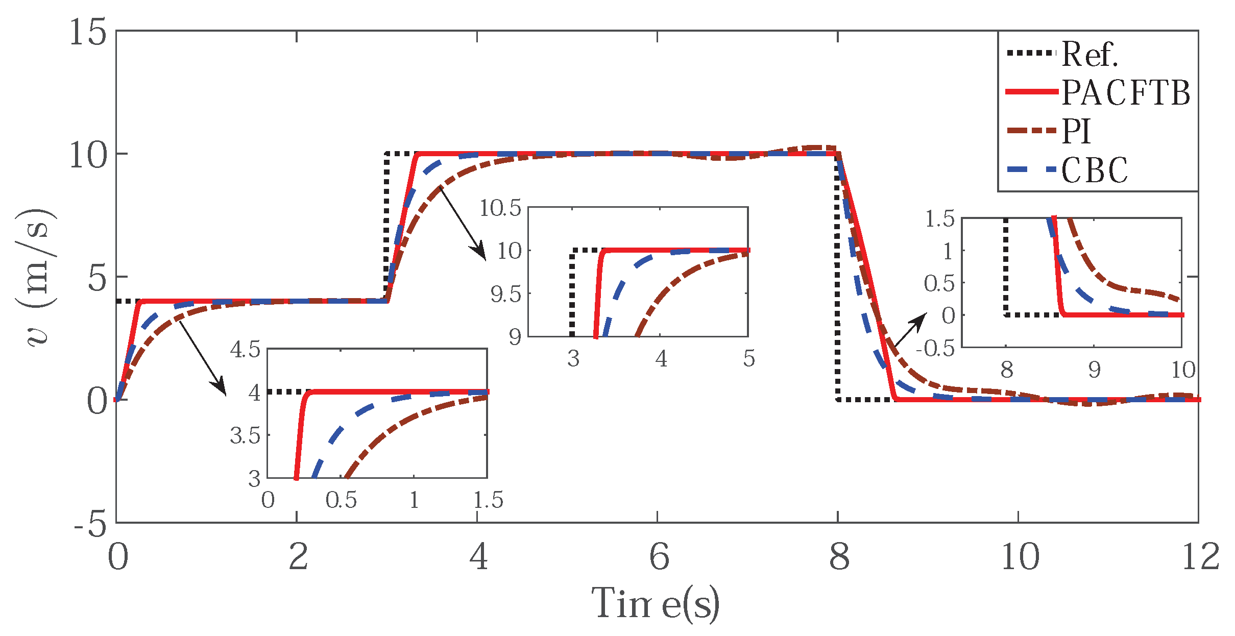
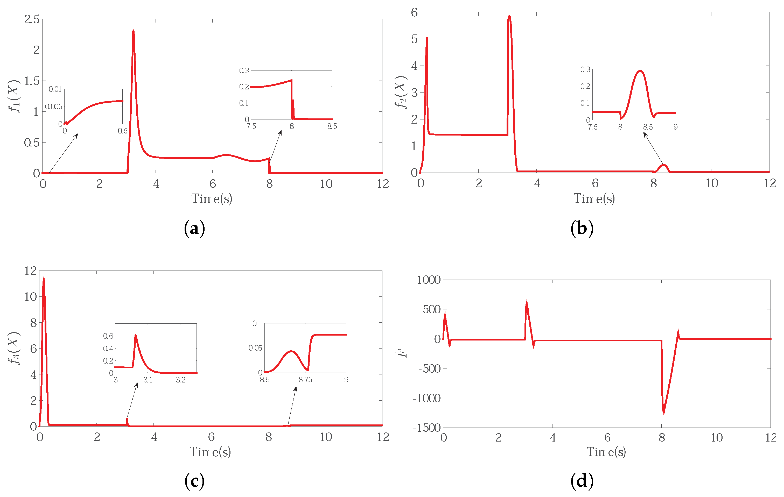
5.1. Simulation Study

In this section, the proposed PACFTB control strategy was simulated in MATLAB/Simulink environment to examine its effectiveness. All the parameters in simulation are listed in

Table 1. Parameters of the investigated LIM.

Parameter	Value	Parameter	Value
$R_s(\Omega )$	0.0709	$R_r(\Omega )$	0.1311
$L_s$(mH)	4.8	$L_r$(mH)	4.8
$L_m$(mH)	3.9	M(kg)	351.264
D(kg/s)	40.95	h(m)	0.2
P	4	l(m)	2

based on finite element analysis. The values of parameters of the proposed controller were: $k_1=40$, $k_2=1000$, $k_3$ = 10,000, $k_d=1$, $k_q=1$, ${\gamma }_1=0.1$, ${\gamma }_2=0.1$, ${\gamma }_3=0.1$, ${\gamma }_4=5\times {10}^6$, $m_1=0.001$, $m_2=0.001$, $m_3=0.001$, $m_4=0.001$, $p_1=p_2=5$ and $q_1=q_2=3$. The values of parameters in command filter were chosen as: $\xi =0.707$, ${\omega }_n=300$, the magnitude and rate constraints were 200 A and 20,000 A/s. As shown in Figure 3, the designed fuzzy membership functions were: ${\mu }_i^j=exp\left[-{\left(x+l\times 2\right)}^2/7\right]$, where $l\in Z$ and $l\in \left[-2,2\right]$. The initial values of vector $W_i(i=1,2,3)$ were defined as $W_i=\underset{5^2}{(\underbrace{0.1,0.1,\dots ,0.1})}$. Notice that all the state variables input to the FLS should be included in fuzzy membership functions. That is to say, all the state variables input to the FLS must be normalized.

In order to test the effectiveness of the proposed PACFTB, the conventional command-filtered backstepping controller (CBC) and PI controller were applied as comparisons to demonstrate the better performance of the designed controller. In simulation, the given d-axis current is 80 A, and the given velocity was set as follows:

$$v_1^d=\left\{\begin{array}{cc}4,\hfill & 0\le t<3\hfill \\ 10,\hfill & 3\le t<8\hfill \\ 0,\hfill & 8\le t<14\hfill \end{array}\right.$$

Meanwhile, external disturbances $F_L=200sin\left(\pi t\right)$ were added in 6 s. The signal curves in the simulation are shown in Figure 4, Figure 5, Figure 6, Figure 7, Figure 8 and Figure 9. By comparing the diagrams of Figure 4 and Figure 5, the PACFTB had faster convergence than CBC and PI controller, which declared the better dynamic performance of PACFTB. In addition, it can be found that PACFTB had better static and dynamic performance than CBC and PI controllers when external load disturbance changed. From the point of view of indices, the response time of our designed controller was $87.5\%$ shorter than that of PI controller, and $83.3\%$ shorter than that of traditional CBC controller. Moreover, the chattering rate of PI caused by external load disturbances was about $2.5\%$ while that of PACFTB is nearly $0.05\%$, which expressed the better performance of PACFTB as well.

Figure 6 shows the d-axis current, which can imply that the proposed controller could stabilize magnetic field. The input and output signals of the command filter are shown in Figure 7, which shows that the output signal $i_{qs}^c$ could effectively track the input signal $i_{qs}^d$ availably and we could get the differential of the input signal directly from the output of the filter. At the same time, by the use of constraint command filter, the output signal was well bounded. The compensator signal is shown in Figure 8, which compensated for the inherent error of the command filter so that the input saturation problem was figured out.

The output signal of FLS is shown in Figure 9a–c. Because of the FLS, it had more extensive and practical significance than CBC and PI controller in practical application without the need of model parameters, and its control performance was obviously better than them in practice. The adaptive disturbance estimation is shown in Figure 9d.

The simulation verified the advanced nature of the designed controller. When the system parameters, model information and external disturbance could not be accurately obtained, the LIM could still track the reference speed precisely via the proposed PACFTB controller. In addition, the controller also kept the system in good working condition when there were unknown parameters and external disturbances.

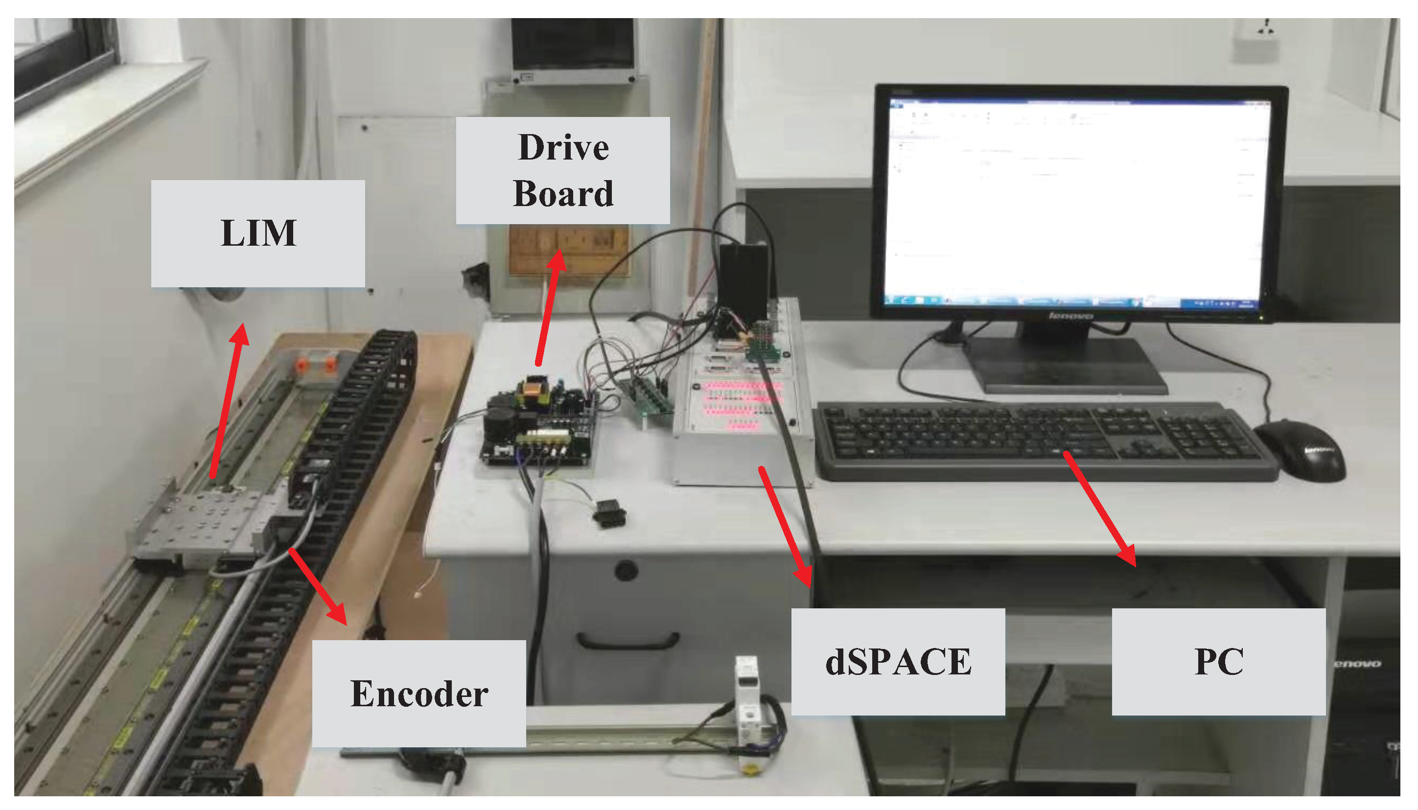
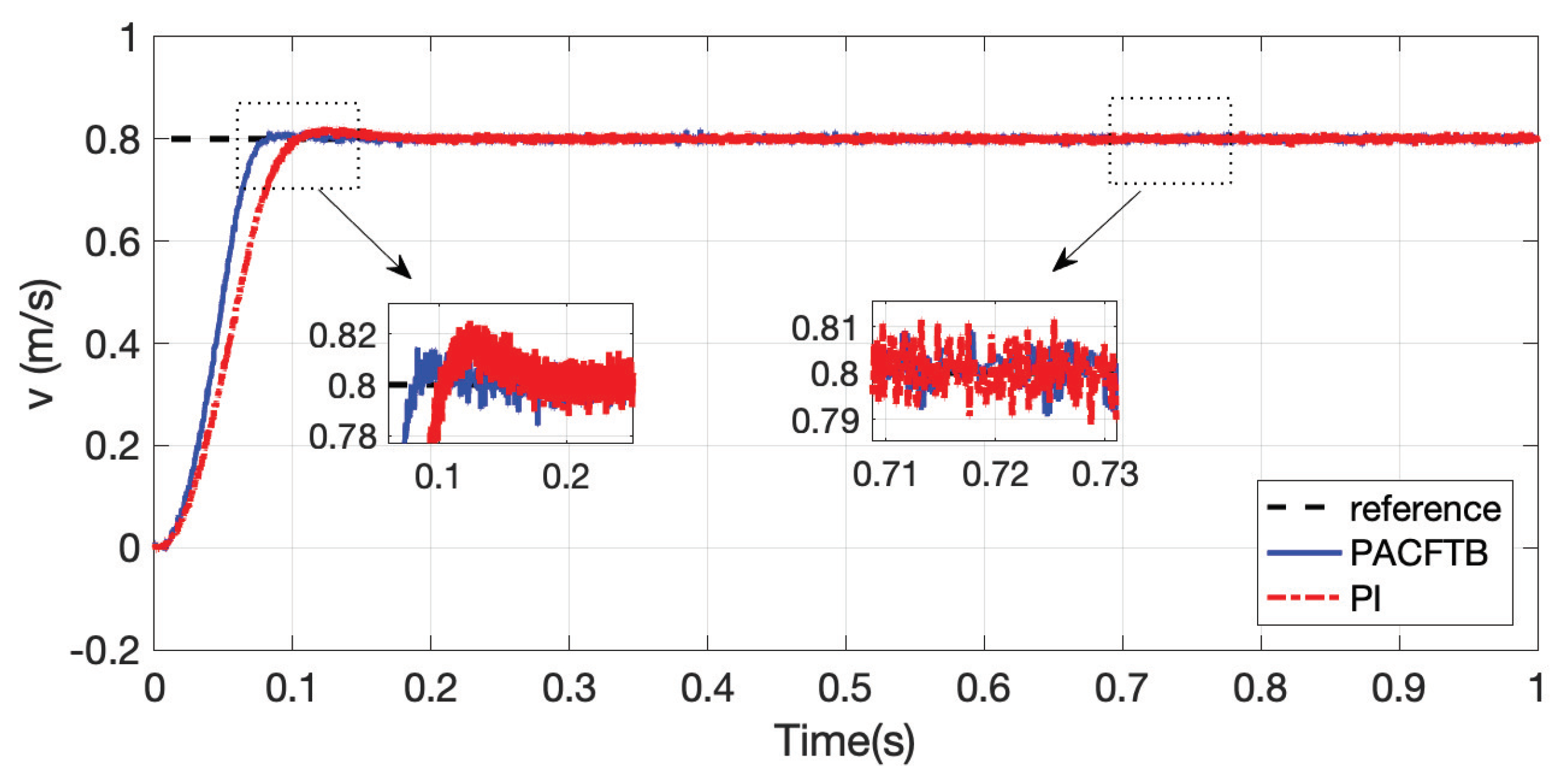
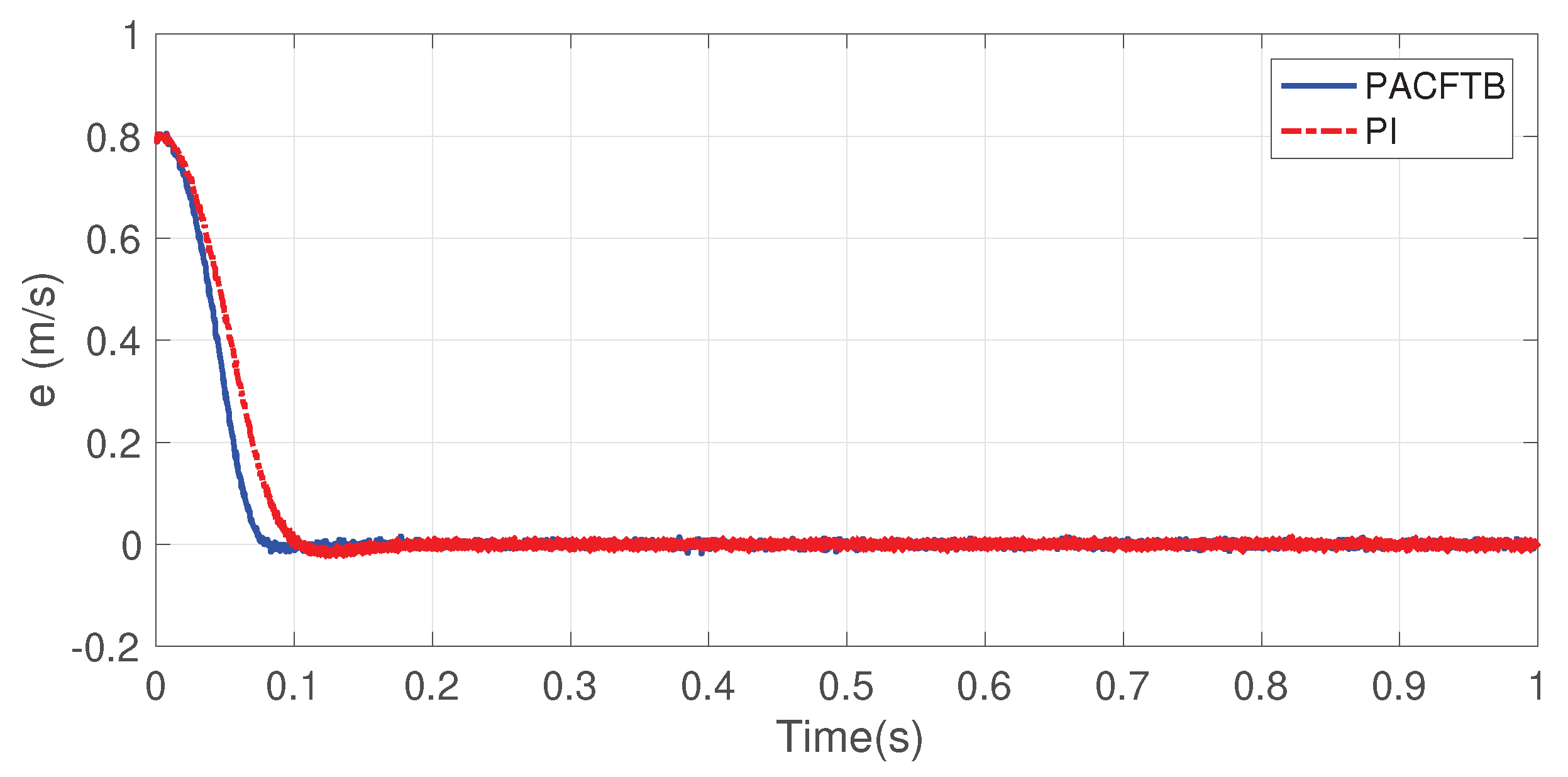
5.2. Experiment Study

Apart from the simulation study, the proposed PACFTB control strategy was also verified in hardware experiment platform based on dSPACE DS1104 control board, which is shown in Figure 10. As can be seen from Figure 10, the platform contained a LIM with encoder, a drive board, a dSPACE DS1104 control board and a PC. When the experiment platform began to operate, the Simulink model of the proposed controller was compiled and loaded to the control board which realized the function of calculation and generation of three-phase PWM signals. The deadband was set as 5 μs and the sample period of speed and current control was 400 μs and 200 μs, respectively.

The desired speed was set as 0.8 m/s and the control objective was to track the desired speed with quick response and little error. The parameters of the controller were set as: $k_1=2000$, $k_2=200$, $k_3=700$, $k_d=k_q=1$, ${\gamma }_1={\gamma }_2={\gamma }_3=0.2$, ${\gamma }_4=5\times {10}^6$, $m_1=m_2=m_3=m_4=0.001$.

Based on the adjustment parameters, the control performance could be achieved, which is shown in Figure 11 and Figure 12. It is shown in Figure 11 that the speed of PACFTB tracked the reference well with quick response and little tracking error. In contrast, the PI control was applied to the experiment as well for speed tracking of LIM. It can be seen that the speed under PI control reached the reference first after 0.1 s while the speed under PACFTB mae it before 0.1 s, which showe better dynamic performance of the proposed PACFTB controller. Furthermore, the chattering at the stable state of PI control was a little more than that of PACFTB controller, which demonstrated better static performance of the proposed PACFTB controller. Thus, the proposed PACFTB control strategy possessed sound static and dynamic performance according to the discussion of experimental results.

6. Conclusions

In this paper, considering the uncertain parameters and external load disturbances in the LIM, the PACFTB controller is designed for the LIM with end effects, which achieves the precise control of the LIM’s velocity. Concretely, the steady state tracking precision and response speed of the system are improved and the system converges at a finite time using the proposed controller. The following conclusions can be drawn.

• The problem of insufficient modeling, unknown nonlinear components and uncertain parameters in the LIM is solved by the FLS combined with an adaptive law.
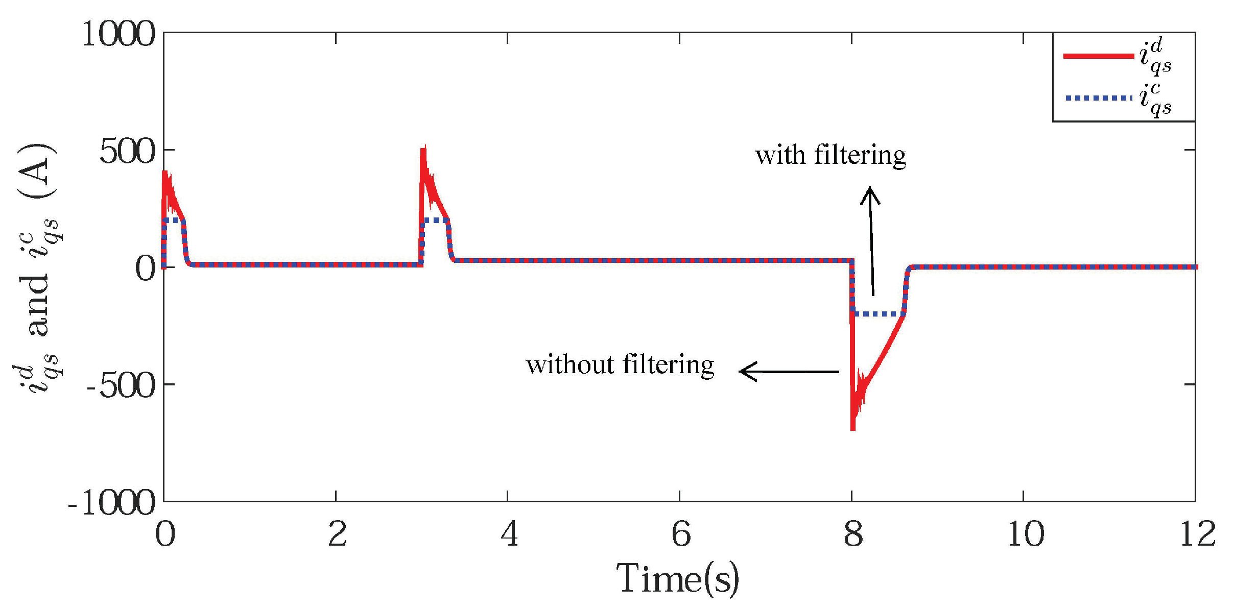
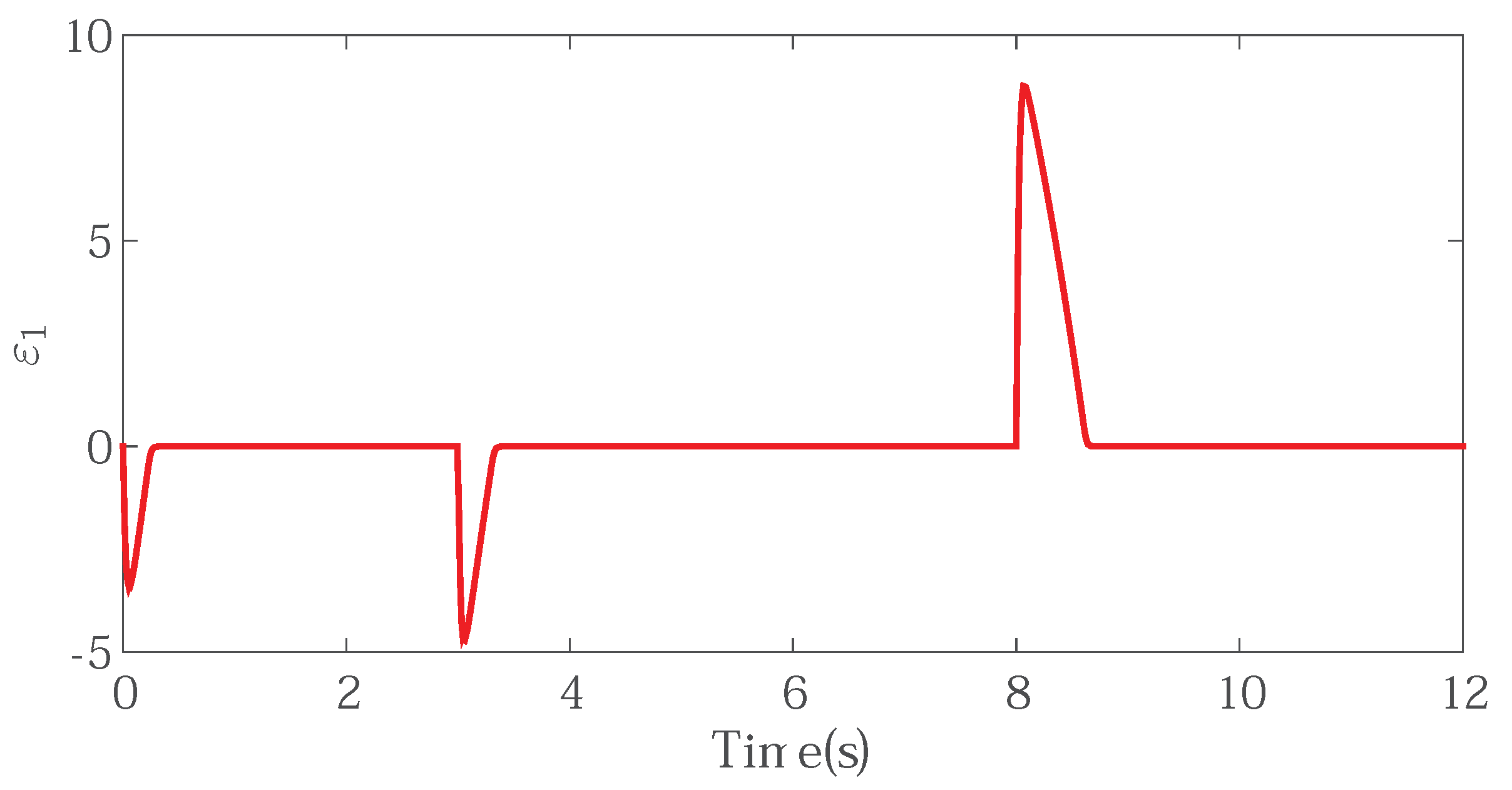
• The introduction of the command filter solves the differential expansion problem in the conventional backstepping algorithm, and the inherent filter error is compensated via the proposed compensation algorithm.
• The introduction of projection operator guarantees the boundedness of estimated parameters and FLS.
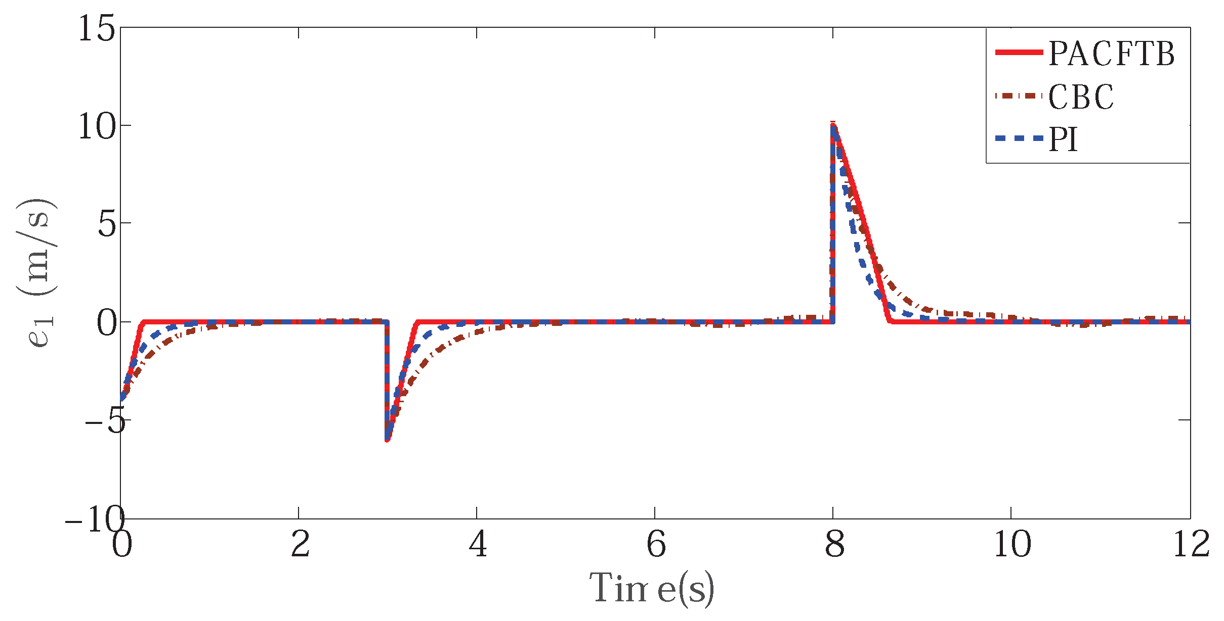
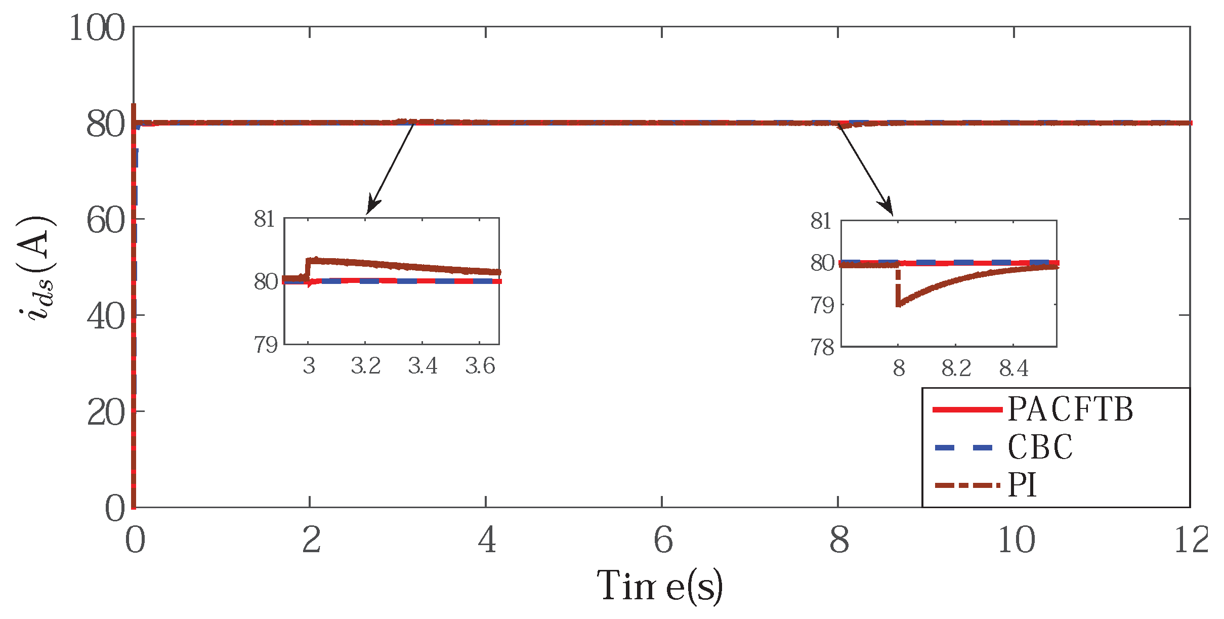
• The simulation results and experimental results indicate that the proposed PACFTB control strategy has remarkable speed tracking performance of the LIM with end effects.

In the future work, the sensor fault or actuator fault would be considered and the corresponding control strategy would be investigated.

References

1. Li, J.Q.; Li, W.L.; Deng, G.Q.; Ming, Z. Continuous-behavior and discrete-time combined control for linear induction motor-based urban rail transit. IEEE Trans. Magn. 2016, 52, 1–4. [Google Scholar] [CrossRef]
2. Ravanji, M.H.; Nasiri-Gheidari, Z. Design optimization of a ladder secondary single-sided linear induction motor for improved performance. IEEE Trans. Energy Convers. 2015, 30, 1595–1603. [Google Scholar] [CrossRef]
3. Yan, L. The linear motor powered transportation development and application in China. Proc. IEEE 2009, 97, 1872–1880. [Google Scholar]
4. Accetta, A.; Cirrincione, M.; Pucci, M.; Vitale, G. Neural sensorless control of linear induction motors by a full-order Luenberger observer considering the end effects. IEEE Trans. Ind. Appl. 2013, 50, 1891–1904. [Google Scholar] [CrossRef]
5. Benmohamed, F.; Bousserhane, I.; Kechich, A.; Bessaih, B.; Boucheta, A. New MRAS secondary time constant tuning for vector control of linear induction motor considering the end-effects. COMPEL Int. J. Comput. Math. Electr. Electron. Eng. 2016, 35, 1685–1723. [Google Scholar] [CrossRef]
6. Creppe, R.C.; Ulson, J.A.C.; Rodrigues, J.F. Influence of design parameters on linear induction motor end effect. IEEE Trans. Energy Convers. 2008, 23, 358–362. [Google Scholar] [CrossRef]
7. Karimi, H.; Vaez-Zadeh, S.; Salmasi, F.R. Combined vector and direct thrust control of linear induction motors with end effect compensation. IEEE Trans. Energy Convers. 2015, 31, 196–205. [Google Scholar] [CrossRef]
8. Xu, D.; Huang, J.; Su, X.; Shi, P. Adaptive command-filtered fuzzy backstepping control for linear induction motor with unknown end effect. Inf. Sci. 2019, 477, 118–131. [Google Scholar] [CrossRef]
9. Wang, H.; Liu, Y.C.; Ge, X. Sliding-mode observer-based speed-sensorless vector control of linear induction motor with a parallel secondary resistance online identification. IET Electr. Power Appl. 2018, 12, 1215–1224. [Google Scholar] [CrossRef]
10. Chiang, H.H.; Hsu, K.C.; Li, I.H. Optimized adaptive motion control through an SoPC implementation for linear induction motor drives. IEEE/ASME Trans. Mechatron. 2014, 20, 348–360. [Google Scholar] [CrossRef]
11. Yu, J.; Shi, P.; Dong, W.; Yu, H. Observer and command-filter-based adaptive fuzzy output feedback control of uncertain nonlinear systems. IEEE Trans. Ind. Electron. 2015, 62, 5962–5970. [Google Scholar] [CrossRef] [Green Version]
12. Accetta, A.; Cirrincione, M.; Pucci, M.; Vitale, G. Closed-loop MRAS speed observer for linear induction motor drives. IEEE Trans. Ind. Appl. 2014, 51, 2279–2290. [Google Scholar] [CrossRef]
13. Hung, C.Y.; Liu, P.; Lian, K.Y. Fuzzy virtual reference model sensorless tracking control for linear induction motors. IEEE Trans. Cybern. 2013, 43, 970–981. [Google Scholar] [CrossRef] [PubMed]
14. Liu, Z.; Chen, B.; Lin, C. Adaptive neural backstepping for a class of switched nonlinear system without strict-feedback form. IEEE Trans. Syst. Man Cybern. Syst. 2016, 47, 1315–1320. [Google Scholar] [CrossRef]
15. Krishna, P.V.; Rao, D.N. Obtaining Speed Response of Linear Induction Motor with Fuzzy Logic Controller with End Effect. Int. J. Electr. Electron. Eng. Res. (IJEEE) 2013, 3, 127–134. [Google Scholar]
16. Alonge, F.; Cirrincione, M.; D’Ippolito, F.; Pucci, M.; Sferlazza, A. Robust active disturbance rejection control of induction motor systems based on additional sliding-mode component. IEEE Trans. Ind. Electron. 2017, 64, 5608–5621. [Google Scholar] [CrossRef]
17. Zhang, W.; Xu, D.; Jiang, B.; Pan, T. Prescribed performance based model-free adaptive sliding mode constrained control for a class of nonlinear systems. Inf. Sci. 2020, 544, 97–116. [Google Scholar] [CrossRef]
18. Yang, X.; Li, J.; Dong, Y. A novel non-singular fast terminal sliding mode control of nonlinear systems with uncertain disturbances. Control Theory Appl. 2016, 33, 772–778. [Google Scholar]
19. Tong, S.C.; Li, Y.M.; Feng, G.; Li, T.S. Observer-based adaptive fuzzy backstepping dynamic surface control for a class of MIMO nonlinear systems. IEEE Trans. Syst. Man Cybern. Part B (Cybern.) 2011, 41, 1124–1135. [Google Scholar] [CrossRef]
20. Jiang, B.; Xu, D.; Shi, P.; Lim, C.C. Adaptive neural observer-based backstepping fault tolerant control for near space vehicle under control effector damage. IET Control Theory Appl. 2014, 8, 658–666. [Google Scholar] [CrossRef]
21. Dong, W.; Farrell, J.A.; Polycarpou, M.M.; Djapic, V.; Sharma, M. Command filtered adaptive backstepping. IEEE Trans. Control Syst. Technol. 2011, 20, 566–580. [Google Scholar] [CrossRef]
22. Liu, H.; Pan, Y.; Li, S.; Chen, Y. Adaptive fuzzy backstepping control of fractional-order nonlinear systems. IEEE Trans. Syst. Man Cybern. Syst. 2017, 47, 2209–2217. [Google Scholar] [CrossRef]
23. Xue, L.; Yi, X.; Lin, Y.C.; Drukker, J.W. An approach of the product form design based on gra-fuzzy logic model: A case study of train seats. Int. J. Innov. Comput. Inf. Control 2019, 15, 261–274. [Google Scholar]
24. Xu, D.; Zhang, W.; Shi, P.; Jiang, B. Model-free cooperative adaptive sliding-mode-constrained-control for multiple linear induction traction systems. IEEE Trans. Cybern. 2020, 50, 4076–4086. [Google Scholar] [CrossRef]
25. Kanchanaharuthai, A.; Mujjalinvimut, E. An Improved Backstepping Sliding Mode Control for Power Systems with Superconducting Magnetic Energy Storage System. Int. J. Innov. Comput. Inf. Control 2019, 15, 891–904. [Google Scholar]
26. Sun, G.; Ma, Z. Practical tracking control of linear motor with adaptive fractional order terminal sliding mode control. IEEE/ASME Trans. Mechatron. 2017, 22, 2643–2653. [Google Scholar] [CrossRef]
27. Sun, G.; Ma, Z.; Yu, J. Discrete-time fractional order terminal sliding mode tracking control for linear motor. IEEE Trans. Ind. Electron. 2017, 65, 3386–3394. [Google Scholar] [CrossRef]
28. Feng, Y.; Zheng, J.; Yu, X.; Truong, N.V. Hybrid terminal sliding-mode observer design method for a permanent-magnet synchronous motor control system. IEEE Trans. Ind. Electron. 2009, 56, 3424–3431. [Google Scholar] [CrossRef]
29. Feng, Y.; Han, X.; Wang, Y.; Yu, X. Second-order terminal sliding mode control of uncertain multivariable systems. Int. J. Control 2007, 80, 856–862. [Google Scholar] [CrossRef]
30. Sun, Z.; Zheng, J.; Wang, H.; Man, Z. Adaptive fast non-singular terminal sliding mode control for a vehicle steer-by-wire system. IET Control Theory Appl. 2016, 11, 1245–1254. [Google Scholar] [CrossRef]
31. Wang, J.; Li, S.; Yang, J.; Wu, B.; Li, Q. Finite-time disturbance observer based non-singular terminal sliding-mode control for pulse width modulation based DC—DC buck converters with mismatched load disturbances. IET Power Electron. 2016, 9, 1995–2002. [Google Scholar] [CrossRef]
32. Zheng, X.; Li, L.; Zheng, J.; Feng, Y. Non-singular terminal sliding mode backstepping control for the uncertain chaotic systems. In Proceedings of the 2008 2nd International Symposium on Systems and Control in Aerospace and Astronautics, Shenzhen, China, 10–12 December 2008; IEEE: New York, NY, USA, 2008; pp. 1–5. [Google Scholar]
Figure 1. Structure of linear induction motor (LIM).
Applsci 10 07405 g001
Figure 2. Proposed PACFTB block diagram.
Applsci 10 07405 g002
Figure 3. The fuzzy membership functions.
Applsci 10 07405 g003
Figure 4. LIM speed tracking effect with different controller.
Applsci 10 07405 g004
Figure 5. LIM speed tracking error with different controller.
Applsci 10 07405 g005
Figure 6. The output of d-axis control current.
Applsci 10 07405 g006
Figure 7. The q-axis current without filtering and with filtering.
Applsci 10 07405 g007
Figure 8. The filter compensating signal.
Applsci 10 07405 g008
Figure 9. Adaptive estimation for unknown parameters. (a) The estimation of f 1 ( X ) ; (b) The estimation of f 2 ( X ) ; (c) The estimation of f 3 ( X ) ; (d) The estimation of load disturbance.
Applsci 10 07405 g009
Figure 10. Hardware experimental platform based on dSPACE.
Applsci 10 07405 g010
Figure 11. Speed tracking performance of LIM.
Applsci 10 07405 g011
Figure 12. Speed tracking error of LIM.
Applsci 10 07405 g012