A Robotic Calibration Method Using a Model-Based Identification Technique and an Invasive Weed Optimization Neural Network Compensator

Abstract

The study proposed a robotic calibration algorithm for improving the robot manipulator position precision. At first, the kinematic parameters as well as the compliance parameters of the robot can be identified together to improve its accuracy using the joint deflection model and the conventional kinematic model calibration technique. Then, an artificial neural network is constructed for further compensating the unmodeled errors. The invasive weed optimization is used to determine the parameters of the neural network. To show the advantages of the suggested technique, an HH800 robot is employed for the experimental study of the proposed algorithm. The improved position precision of the robot after the experiment firmly proves the practicability and positional precision of the proposed method over the other algorithms in comparison.

1. Introduction

Robot manipulators are widely used in industry to attain many duties such as welding, painting, pick and place task, etc. The construction of robot manipulators is characterized using their kinematic model parameters. However, experience has shown that industrial manipulators have much greater repeatability than accuracy [1]. Therefore, the utility of robot manipulators would be significantly enhanced if they were made to be as accurate as they are repeatable. In producing and assembly, many errors arise that could not be taken into account by the nominal geometric model. For that reason, there is a demand to create model-based robotic calibrations that depend on an error model that symbolizes the connection between the errors of geometric parameters and the end effector positioning errors. The kinematic calibration method has been widely researched by numerous studies [2,3,4,5,6,7,8,9,10,11,12,13] to describe the proper geometric model. Denavit, Hartenberg et al. proposed one of the most fundamental calibration methods that is widely used. The DH model is based on homogenous transformation matrices. The model is a description of the kinematic relations between the links of a kinematic chain connected by 1 degree-of-freedom lower pair joints [6,7,8]. There are also other methods such as the zero-reference position model that is proposed by Gupta et al., which has been widely used by many studies [9,14,15]. Another fundamental model-based calibration method is the complete and parametrically continuous (CPC) model, which relies on the singularity-free line representation by Zhuang et al. [10,11]. Park and Okamura [12] employed the product of exponentials (POE) error model to robot calibration. This model has been adopted by several researchers [4,13]. There have been some attempts to replace the least square estimation with the Kalman filter, particle filter, fuzzy theory, etc. [16,17,18]. However, those attempts did not seem to be very effective.

In addition, the kinematic errors are not the only source of robot manipulator errors. Whitney et al. [19] used a PUMA 560 robot to determine that the most significant error sources for the robot were several nongeometric errors. Judd and Kasinski [20] studied an AID-900 robot and found that the geometric errors were responsible for approximately 95% of the measured error. Jean et al. [21] and Becque [22] reported that flexibility in joints and in links is responsible for 8–10% of the total position and orientation errors. Therefore, more recently, researchers have been devoted to the identification of compliance errors as well as kinematic errors in industrial robots [5,20,23]. Jian Zhou and Hee-Jun Kang [5] proposed a method for simultaneously identifying the kinematic and compliance parameter of the robot. The model-based calibration has been widely applied due to its fast computing and knowledge of error sources [5,24,25]. However, the accuracy of the model-based calibration method is dependent on the model accuracy. It is practically impossible to create a model that contains all the sources committing to the end effector errors. Some error sources such as gear backlash, temperature variation, and other errors are difficult to model correctly and completely.

To archive further accuracy, nongeometric calibration has been widely studied for compensating for the sources of errors that could not be taken into account by geometric calibration [17,21,26,27,28,29,30,31,32,33]. The conventional back-propagation neural network (BPNN) [34] is widely adopted by researchers [35] for compensating the unmodeled errors to increasing the precision of the robot. In robotic calibration processing, BPNN is usually employed to construct the relationship between the end effector position and the corresponding joint angle configuration [36,37,38,39]. However, the conventional BPNN has some drawbacks such as getting stuck in local minima and slowing convergence [40]. To overcome these drawbacks, some heuristic algorithms have been used for training the network [41,42,43,44,45]. One among them is the Invasive Weed Optimization (IWO) algorithm.

In 2016, Mehrabian et al. presented the Invasive Weed Optimization (IWO) algorithm [46]. This method is motivated by the spreading of weeds to find a suitable place for expanding and breeding. The technique is characterized by fast convergence for global optimization. Based on the properties of IWO, this algorithm is employed for optimizing the parameters of a neural network to reduce its cons such as a high dependence on input data. Furthermore, the IWO prevents the neural network from falling to local minima.

This work proposed a new calibration method that includes the model-based calibration technique and unmodeled calibration method. At first, the kinematic and compliance parameters are simultaneously determined by a model-based calibration method [5]. Then, the method needs to compensate for some unmodeled errors that cannot be ignored such as friction, mechanical transmission error, and thermal expansion. A suggested neural network optimizing by IWO is used to compensate the residual positional errors. It should be noted here that the proposed method is a combination of model-based and artificial neural network (ANN) methods that used the IWO technique to determine the weight and bias. Meanwhile, most of the ANN-based technique is applied after the kinematic calibration. This calibration method simultaneously calibrates both the kinematic errors and joint compliances. After the simultaneous calibration, the IWO-NN-based compensation is accomplished for the unmodeled nongeometric errors. By using the IWO neural network, the proposed calibration method seems to reach the global minima easily. Therefore, the IWO neural network can be said to have better convergence capability than the traditional backpropagation NN. Finally, a HH800 robot is employed for the experimental study of the proposed algorithm to compare with four other calibration methods, including the conventional kinematic calibration method (KM), as well as the simultaneous identification of joint compliance and kinematic parameters method (SKCM), and the combination of an NN compensator and SKCM method (NN-SKCM). The advantages of the method have been shown: the enhanced position accuracy of the manipulator after the calibration confirms the feasibility and greater positional accuracy over the other calibration methods. Additionally, the adopted IWO neural network has better convergence capability than the back-propagation neural network in this calibration process. This advantage makes the proposed method more feasible in real offline programming environments.

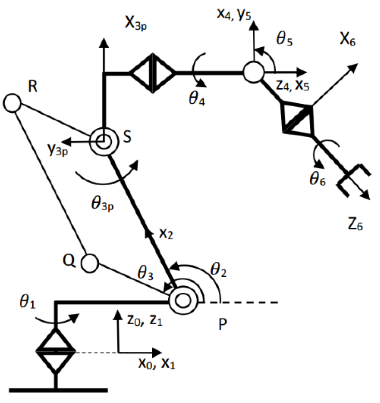
2. Kinematic Model of the HH800 Robot

The HH800 robot [36] model is given in

Table 1. Nominal D-H parameters of a Hyundai robot HH800.

D-H Parameters of the Main Open Chain
i	αi−1 (deg)	ai−1 (m)	βi−1 (deg)	bi−1 (m)	di (deg)	θi (deg)
1	0	0	0	0	0	θ1
2	90	0.515	-	-	0	θ2
3	0	1.6	0	-	0	θ3
4	90	0.35	-	-	1.9	θ4
5	−90	0	-	-	0	θ5
6	90	0	-	-	0.445	θ6
T	-	−0.45	-	0.11	0.930	-
D-H Parameters of the Main Open Chain
L5 (m)		0.8	L4 (m)	1.6	L3 (m)	0.8

and Figure 1. The homogeneous transformation matrix from the robot base frame to the end effector frame can be computed by:

$${}_E{}^{0}T={}_1{}^{0}T\left({\theta }_1\right){}_2{}^{1}T\left({\theta }_2\right){}_{3p}{}^{2}T\left({\theta }_{3p}\right){}_4{}^{3p}T\left({\theta }_4\right){}_5{}^{4}T\left({\theta }_5\right){}_6{}^{5}T\left({\theta }_6\right){}_E{}^{6}T.$$

(1)

The homogenous transformation matrix from the robot 6th frame to the end effector frame:

$${}_E{}^{6}T=T{r}_X\left(a_6\right)T{r}_Y\left(b_6\right)T{r}_Z\left(d_6\right).$$

(2)

The passive joint position ${\theta }_{3p}$ is formed from the joints ${\theta }_2$ and ${\theta }_3$ as follows [36,47]:

$${\theta }_{3p}={\theta }_3-{\theta }_2-90$$

(3)

3. Simultaneous Joint Stiffness and Kinematic Parameters

In a robot static configuration, a robot joint torque causes a twist deformation about a rotation shaft (that represents the entire drive train from the motor to the associated robot link). Therefore, the shaft can be considered as a torsional spring in the compliance modeling. This study investigates the characteristics of a torsion spring because they are related to modeling of rotational joint compliance. The characteristics of torsion springs are basically presented by non-linear functions: for example, $\tau =k_1\ast \Delta {\theta }_c+k_2\ast {\left(\Delta {\tau }_c\right)}^3$, where $\tau$ is the spring torque, $\Delta {\theta }_c$ is the spring rotational deformation, and k₁ and k₂ are the coefficients. When the robot joint deformation is small, the linear part becomes dominant. Now, we can assume that the functional relationship between the joint torque and its deformation is linear in this calibration process.

Assuming that the compliance of the robot links is small and can be neglected, therefore, the elastic errors are mostly dependent on the compliance of joints under the link self-gravity and external payload. Accepting that the robot joint deformations can be expressed by a linear function of the joints torque, the deformation of the ith joint can be expressed by the effective torques ${\tau }_i$:

$$\Delta {\theta }_{ci}=\frac{{\tau }_i}{k_i}={\tau }_i{c}_i$$

(4)

where $k_i$ is the joint stiffness value of the ith joint.

The Cartesian position errors due to small joint deflections can be modeled as:

$$\Delta P_c=J_{\theta }\Delta {\theta }_c=\left(J_{\theta }\tau \right)C$$

(5)

The compliance vector is denoted by $C={\left[\begin{array}{cc}\begin{array}{cc}{c}_1& c_2\end{array}& \begin{array}{cc}\cdots & c_n\end{array}\end{array}\right]}^T$. The deflection vector is $\Delta {\theta }_c={\left[\begin{array}{cc}\begin{array}{cc}\Delta {\theta }_{c1}& \Delta {\theta }_{c2}\end{array}& \begin{array}{cc}\cdots & \Delta {\theta }_{c\mathrm{n}}\end{array}\end{array}\right]}^T$. At the equilibrium position, $\tau =diag\left({\tau }_1,{\tau }_2,\cdots ,{\tau }_n\right)$ is the effective torque of robot joints. The real position vector of the robot end-effector can be expressed as:

$$P_{real}=P_{kin}+\Delta P_{kin}+\Delta P_c+\Delta P_{extra}$$

(6)

where $P_{kin}$ is the end effector position that is calculated by the kinematic parameters. $\Delta P_{kin}, \Delta P_c,$ and $\Delta P_{extra}$ are the position errors due to the kinematic parameter errors, joint deflections, and the residual errors due to the unmodeled sources, respectively. Jian Zhou and Hee-Jun Kang [5] presented a method for simultaneous identifying the kinematic and compliance parameter of a robot:

$$\begin{array}{ccc}\Delta X& =& \Delta P_{kin}+\Delta P_c\hfill \\ & =& J\Delta \varphi +J_{\theta }\Delta {\theta }_c\hfill \\ & =& J\Delta \varphi +J_{\theta }C\tau \hfill \\ & =& \left[\begin{array}{cc}J& J_{\theta }\tau \end{array}\right]\left[\begin{array}{c}\Delta \varphi \\ C\end{array}\right]\hfill \\ & =& J_{\Phi }\Delta \Phi \hfill \end{array}$$

(7)

where $\Delta X$ is a (3 × 1) vector of three position errors of the robot end-effector. $J$ is a (3 × p) matrix that relates the column vectors $\Delta X$ and $\Delta P_{kin}$ (p = 27 is the total number of kinematic parameters). By using the least-square method, the kinematic and joint compliance parameter can be computed at the same time.

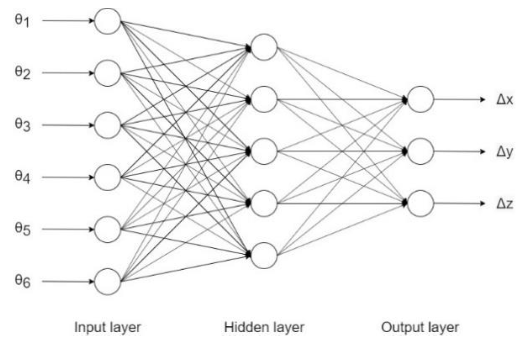
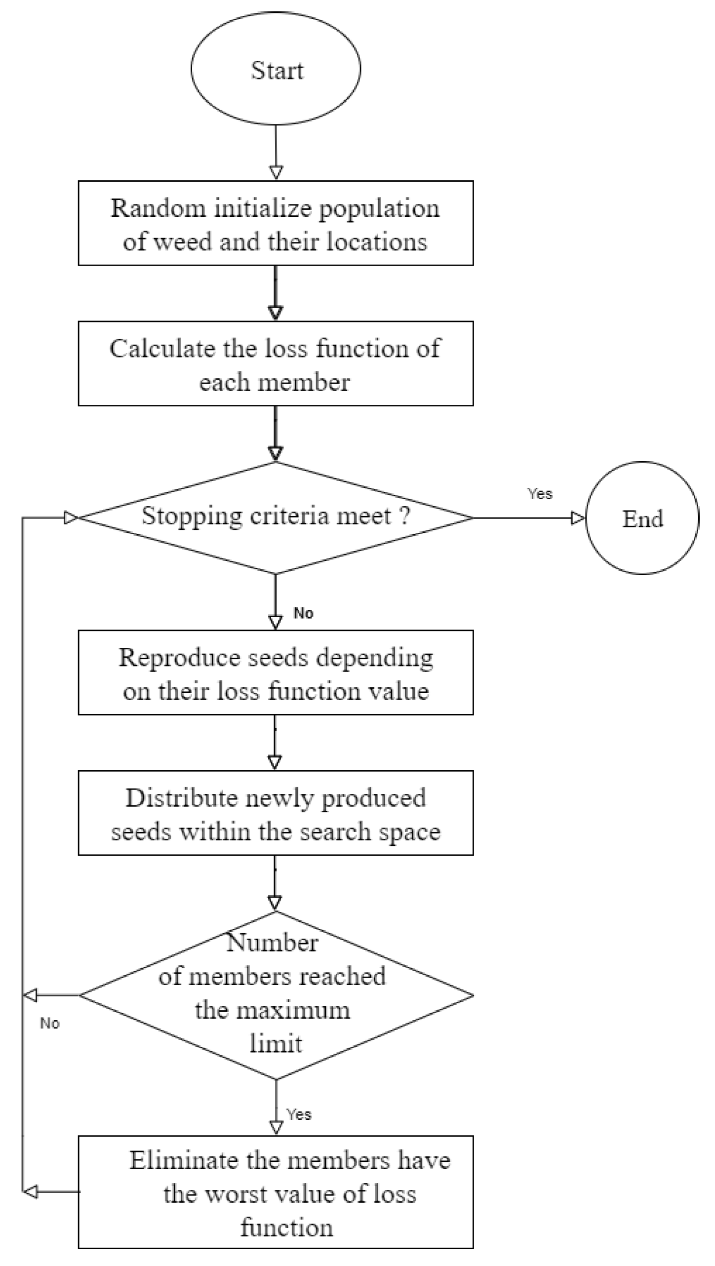
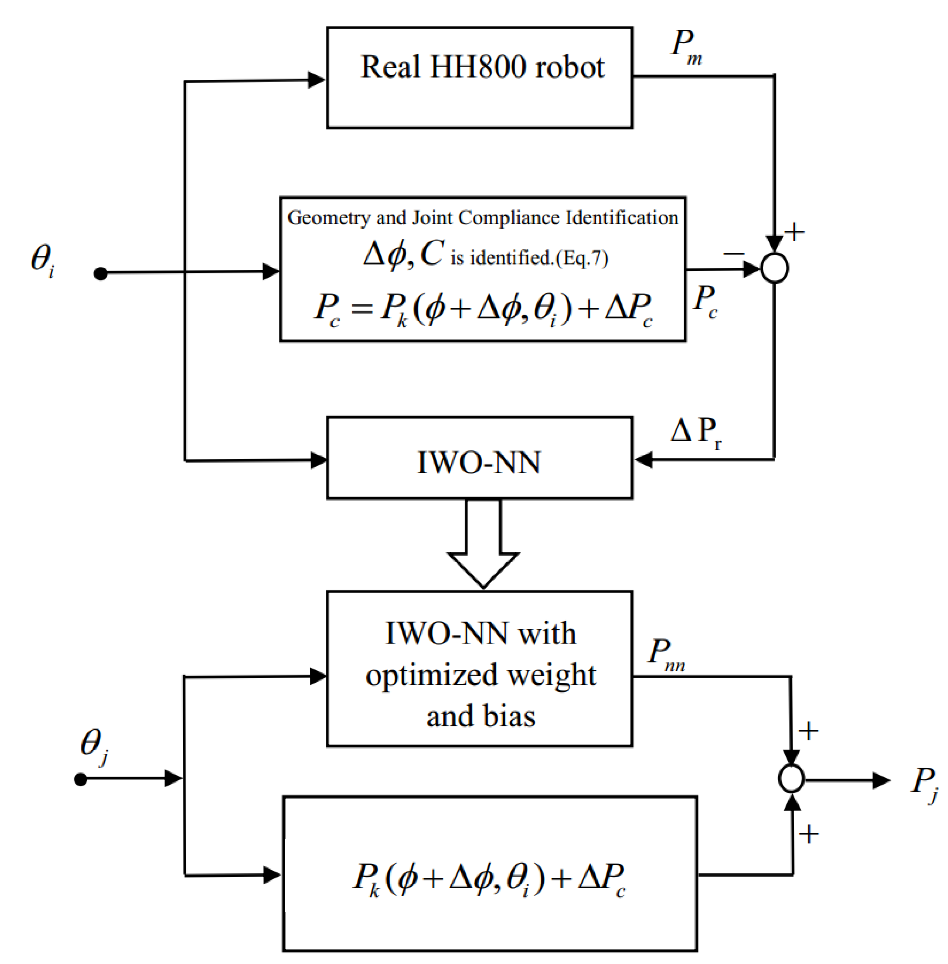
4. IWO-NN Errors Compensator Technique

In Equation (6), the position errors $\Delta P_{extra}$ are still large after applying the algorithm of simultaneous identification of joint compliance and kinematic parameters. This occurred because of some unmodeled sources such as friction, thermal extension, mechanical transmitting errors, which are hardly considered in geometric calibration. To decrease these unmodeled errors, a nongeometric compensator should be carried out for compensating. In this study, an IWO-NN errors compensator is taken to eliminate the residual positional errors. The method is fully described as follows.

First, the robot geometry error $\Delta \varphi$ and joint compliance parameter $C$ are identified together (Equation (7)) using the least squares method. The total positional error vector is denoted by $\Delta P$ (3 × 1):

$$\Delta P=P_m-P_c=\Delta P_{kin}+\Delta P_c+\Delta P_{extra}$$

(8)

where $P_m,P_c$ indicate the positions of the end effector by measuring and computing. $\Delta P_{kin},\Delta P_c$ are the kinematic error and compliance error that are calculated by applying the method in Ref. [5]. The residual position error after the modeled-based calibration process is $\Delta P_r$. Here, the IWO-NN is hired to compensate the residual error $\Delta P_r$.

$$\Delta P_r=\Delta P-\Delta P_{kin}-\Delta P_c$$

(9)

The IWO-NN containing six inputs representing the joint configurations is ${\theta }_n=\left[{\theta }_1,{\theta }_2,\cdots ,{\theta }_6\right]$. There are five nodes in the hidden layer (Figure 2). The tag-sigmoid is selected as the activate function for the hidden layer as follows [36]:

$$z=tansig\left(a\right)=\frac{2}{1+e^{-2a}}.$$

(10)

Three outputs of the NN have the linear activation function. The outputs of the NN are used for compensating the residual errors $\Delta P_r$.

The error in the output layer is

$$e=\Delta P_r-P_{nn}$$

(11)

where $P_{nn}$ is the output of the neural network.

The mean square error is calculated as follows:

$$E=\frac{1}{m}{\displaystyle \sum }_{k=1}^m{e}_k^2$$

(12)

where m = 3 represents the three dimensions of the end-effector position. The IWO is a recently proposed population-based heuristic optimization algorithm that mimics the spreading of weeds to find a suitable place for expanding and breeding [46]. IWO has four main stages: (i) initialization, (ii) reproduction, (iii) space distribution, and (iv) ranking and selection.

(i) Initialization: The population of solution is generated. The seeds are randomly distributed over all the space problem. The number of seeds is chosen.

(ii) Reproduction: In this step, every seed reproduces the next generation. The number of every seed’s heir depends on its fitness in the community. If the seed has a good fitness, it will produce more seeds than another seed that has a worst fitness in the society.

(iii) Space Distribution: This is the progress by which the offspring are randomly spread over all the searching space. The spreading process is made to distribute the offspring close to their parents’ location. Therefore, the seeds with lower fitness in the population are deleted over time. The distribution function is described as below:

$${\sigma }_{iter}=\frac{{\left(ite{r}_{max}-iter\right)}^n}{{\left(ite{r}_{max}\right)}^n}\left({\sigma }_{initial}-{\sigma }_{final}\right)+{\sigma }_{final}$$

(13)

where ${\sigma }_{iter}$ is the standard deviation (SD) at the present step, $ite{r}_{max}$ is the maximum number of iterations before stopping the algorithm, ${\sigma }_{initial}$ is the initial value of the SD, ${\sigma }_{final}$ is the final value of the SD, and $n$ is the non-linear modulation index.

(iv) Ranking and Selection: When the maximum number of populations in the colony is hit, all the seeds are evaluated, including new seeds and their producers. The unqualified fitness seeds will be eliminated.

In this work, the IWO is introduced for optimizing the weights and biases of an NN. The optimizing process is described by the flowchart in Figure 3.

Assume that $X_i=\left\{x_i{}_1,x_i{}_2,\cdots ,x_i{}_n\right\}$ is the ith member that contains the weights and biases of the NN. An initial population including 10 members is randomly spread over the searching space. The maximum population size is 50. The minimum number of seeds is $S_{min}=0$, and the maximum number of seeds is $S_{max}=5$. The variance reduction exponent is $n=2$ (Equation (13)). The initial value of the SD is ${\sigma }_{initial}=0.05,$ while the final value of the SD is ${\sigma }_{final}=0.0005$. The dimension of member $X_i$ of the population is $i=53$ according to the number of the weights and biases of the fully connected NN, which has six inputs, three outputs, and five hidden nodes.

The loss function is used for evaluating the fitness of member $X_i$ of the population:

$$L{F}_i=l_1\ast mean\left(E_i\right)+l_2\ast max\left(E_i\right).$$

(14)

Here, $E_i$ is the matrix of mean square errors (Equation (12)) of the ith set of NN respectively to 50 inputs and outputs of the calibration data. $l_1=1$; $l_2=0.7$ are the weights that represent the contribution of mean and max function in forming the cost function of each solution i.

By using Equation (14), the number of seeds for member $X_i$ of the population can be calculated:

$$S=floor\left(S_{min}+\left(S_{max}-S_{min}\right)\ast r_i\right)$$

(15)

where $floor$ is the function that rounds to the nearest integer less than or equal to the input number. $r_i$ is the ratio calculated by the following equation:

$$r_i=\frac{L{F}_i-\max \left(LF\right)}{\min \left(LF\right)-\max \left(LF\right)}.$$

(16)

The seed $S_j$ of member $X_i$ can be calculated by

$$S_j=X_i+{\sigma }_{iter}\ast K$$

(17)

using ${\sigma }_{iter}$ (Equation (15)). $K$ is a matrix that has the same dimension as $X_i$. Every element of $K$ is a random number between 0 and 1. For speeding the process, the values of elements of $S_j$ are bounded. The lower and upper bounds are −1.7 and 1.7, respectively.

After this process, all the seed $S_j$ of member $X_i$ are merged into the population and considered members of the population. If the number of members overcomes the maximum population size, the worst members having the highest valued loss function are eliminated. Then, the processing is repeated again until it reaches the maximum iteration or one of the members archives the desired loss function value.

Figure 4 shows the flowchart of the proposed method.

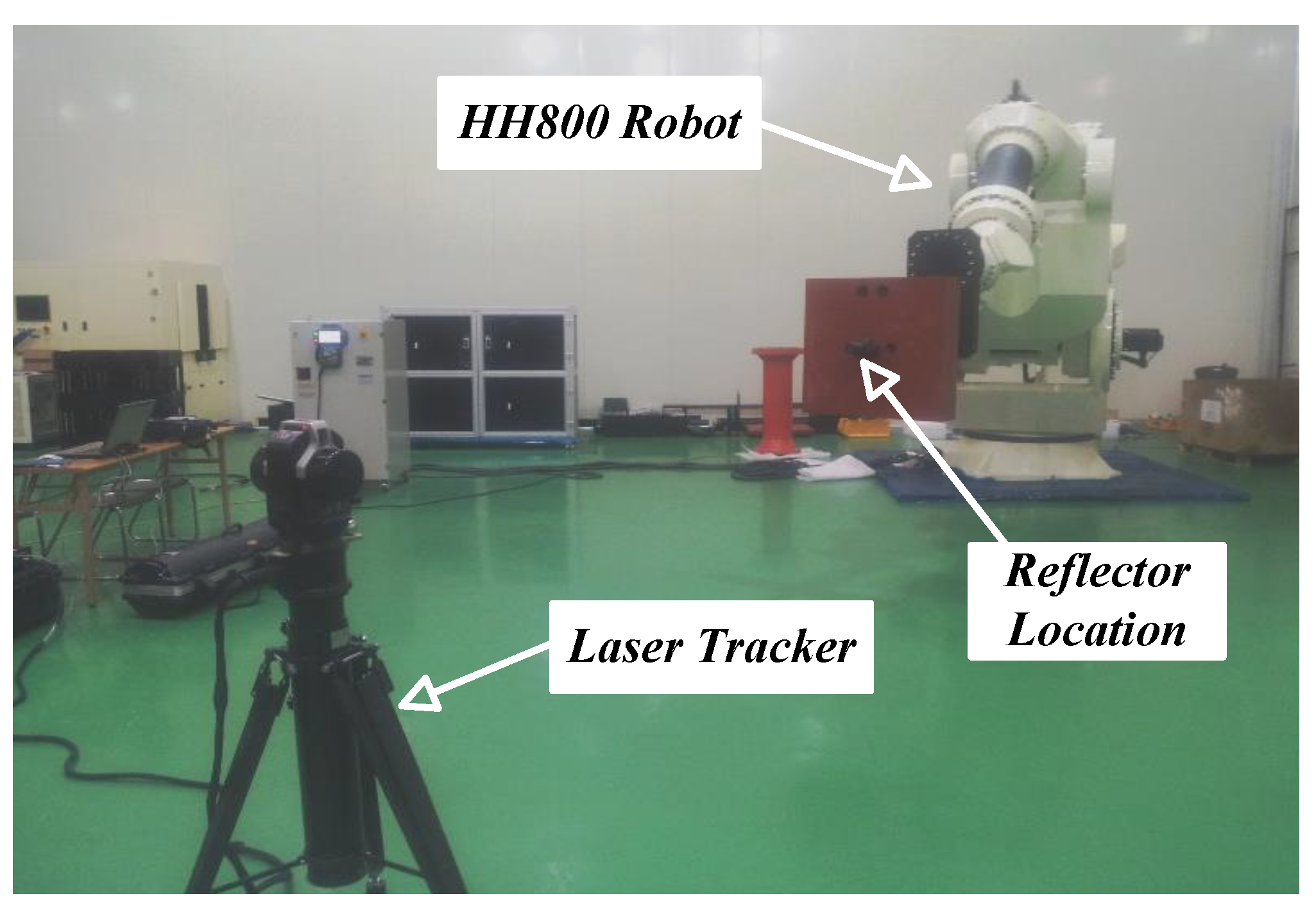
5. Experiment and Validation Results

An HH800 robot is employed to examine the proposed method to clarify the effectiveness and practicability of it. The proposed method is examined in contrast with the other four methods to show its advantages. To demonstrate the effectiveness of the proposed method (IWO-NN-SKCM) in improving the robot position accuracy, four calibration methods are carried and compared in both the calibration and validation process. The conventional kinematic calibration method (KM) [6], as well as the simultaneous identification of joint compliance and kinematic parameters method (SKCM) [5], and the combination of NN compensator and SKCM method (NN-SKCM) [36] are used in this experiment calibration.

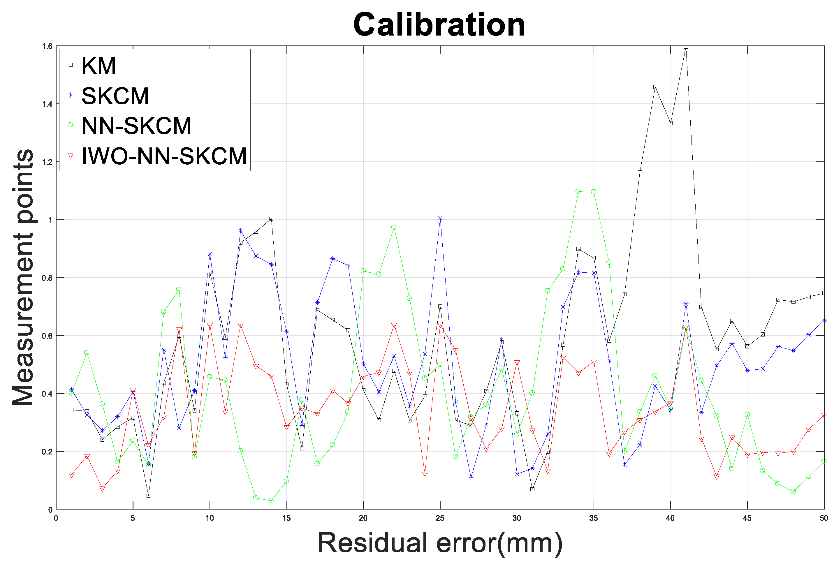
5.1. Experimental Calibration Results

In this experiment, a robot calibration system consists of a Hyundai HH800 robot (6 degree of freedom (d.o.f)) that has one closed-loop actuating mechanism, a 3D point sensing device (API Laser Tracker, measurement accuracy of 0.01 mm/m, repeatability of +/−0.006 mm/m), and an accompanying laser reflector. The reflector is fixed at a particular location of the robot end-effector. The system is arranged as shown in Figure 5.

In order to acquire suitable measurement data for robot parameter identification and IWO-NN training, the robot moves its end-effector to positions such that they entirely cover the workspace. The three-dimensional coordinates of the end points are measured by the Laser Tracker and saved in a computer. At the same time, the associated robot joint readings also are recorded.

These measurements are grouped as follows: A set of 40 robot configurations (Q1) is used for parameter identification and collected over all the workspaces. By using the SKCM method, the kinematic and joint compliance parameters are identified. These parameters are presented in

Table 2. Stiffness identification.

	K2	K3	K4	K5
Stiffness	6.159 × 107	4.388 × 106	3.151 × 106	2.220 × 106

and

Table 3. Identified D-H parameters of Hyundai robot HH800 (“-”: unavailable, “X”: unidentifiable).

D-H Parameters of the Main Open Chain
i	αi−1 (deg)	ai−1 (m)	βi−1 (deg)	bi−1 (m)	di (deg)	θI (deg)
1	0.8752	0.0003	0.006	0.0001	0.0976	0.3468
2	89.9412	0.5157	-	-	0 (X)	−0.8836
3	0.0133	1.5998	0.001	-	−0.0014	−1.2385
4	90.1172	0.3545	-	-	1.8862	3.3033
5	−90.038	0.0002	-	-	4.087 × 10−5	2.5786
6	90.0371	0.0003	-	-	0.445 (X)	0 (X)
T	-	−0.4511	-	0.0111	0.9279	-
D-H Parameters of the Main Open Chain
L5 (m)		0.7996	L4 (m)	1.601	L3 (m)	0.8 (X)

, including four joint compliance parameters and 29 kinematic parameters. Another set (Q2) of 50 robot configurations is also randomly selected to determine the weights and biases of the neural network that has five hidden nodes, six inputs, and three outputs. The reason why we use a different set (Q2) from the first set (Q1) is that the neural network compensator has more general error compensation capability over the entire robot workspace. A set of 50 arbitrary endpoints (Q3) for robot accuracy validation is collected over all the workspaces.

In this calibration progress, the HH800 robot is used to apply four different calibration algorithms.

Table 4. Absolute position accuracy of the HH800 robot (calibration).

	Mean (mm)	Max. (mm)	Std. (mm)
Before calibration	4.5969	6.6664	0.8408
KC	0.5961	1.5967	0.3299
SKC	0.5038	1.005	0.2346
NN-SKC	0.4103	1.0967	0.2814
IWO-NN-SKCM	0.3450	0.6374	0.1624

and Figure 6 demonstrate the results of these calibration methods. Figure 6 provides a visual result of the absolute position errors of each calibration pose using four calibration methods, including the conventional kinematic calibration method (KM), as well as the simultaneous identification of joint compliance and kinematic parameters method (SKCM), and the combination of NN compensator and SKCM method (NN-SKCM). It shows that the position errors generated by the proposed method are the lowest and better converging in comparison with the other methods. By using the IWO-NN SKCM, the mean of errors is reduced from 0.5961 to 0.3450 mm by as much as 42.12% compared to the KM method. This mean of errors is also decreased as much as 31.52% in comparison to the SKCM method (0.5038 mm). In comparison to the NN-SKCM method, the mean of errors result is declined 15.92% (0.4103 mm). The IWO-NN is better than NN-SKCM in reducing the maximum of absolute position errors (41.88%). The proposed method also generates the lowest maximum position error (0.6374 mm) and standard deviation (0.1624 mm).

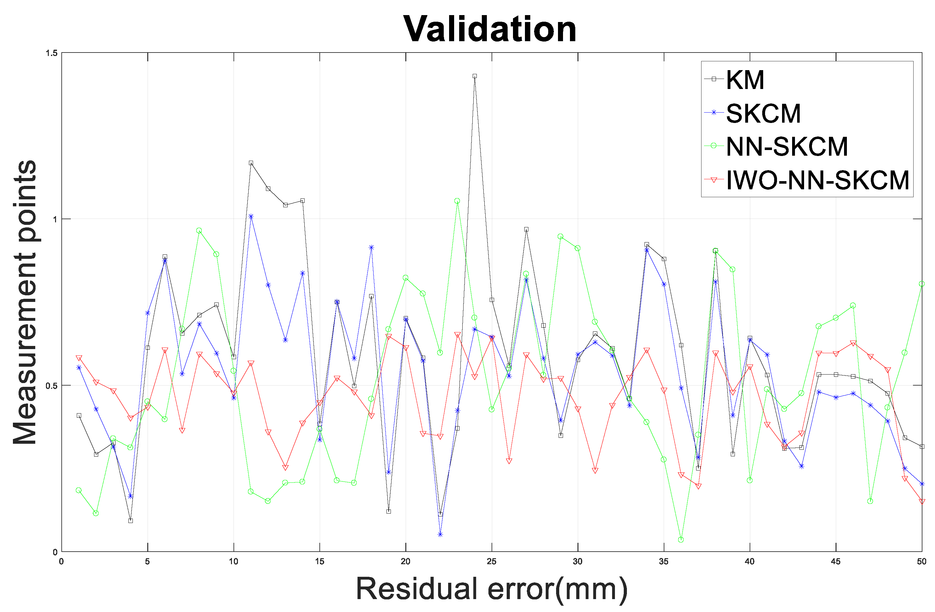
5.2. Experimental Validation Results

The validation process is examined to illustrate the general capability of the suggested calibration technique over the entire robot workspace. In this progress, the set Q3 includes 50 robot configurations of the manipulator that are not used in the calibration process, and it is taken to examine the four different methods. The results of the validation process are demonstrated in Figure 7 and

Table 5. Absolute position accuracy of the HH800 robot (validation).

	Mean (mm)	Max. (mm)	Std. (mm)
Before calibration	4.4266	6.2749	0.6772
KC	0.5981	1.4293	0.285
SKC	0.5458	1.0078	0.2142
NN-SKC	0.5187	1.0532	0.2642
IWO-NN-SKCM	0.4662	0.6538	0.1333

. Figure 7 shows the residual error of 50 poses using four methods in the validation process. It is clear to see from the figure that the proposed method is the best over both the positions used in the calibration process and the general position in the overall workspace.

By using the proposed method, the mean of errors is reduced from 0.5981 to 0.4662 mm by as much as 22.07% better in comparison to the KM method. The mean of errors is also decreased by as much as 26.72% in comparison to the SKCM method (0.5458 mm), and there is a 10.14% decline from the mean of errors by using the NN-SKCM method (0.5187 mm). The proposed method also generates the lowest maximum position error (0.6538 mm) and standard deviation (0.1333 mm).

5.3. Advantages of the IWO-NN Compensator

In this work, the robot configurations are divided into several datasets that are compensated by the NN and the proposed IWO-NN. From this experimental application, the NN appear to be usually fallen into the local minima, and a reinstalling of random weights and bias is required to reach the global minima. On the other hand, the IWO-NN seems to archive the global minima quite efficiently. For that reason, the proposed IWO-NN can be said to have better convergence capability. Moreover, an accuracy consistency of experimental calibration (0.345 mm) and validation (0.4662 mm) confirms the abilities of the suggested calibration method.

6. Conclusions

In this study, a new calibration method with an error compensating IWO neural network is proposed for enhancing the robot positional accuracy of the industrial manipulators. By combining the joint deflection model with the conventional kinematic model of a manipulator, the geometric errors and joint deflection errors can be simultaneously considered to increase its positional accuracy. Then, a neural network is designed to additionally compensate the unmodeled errors, such as friction, mechanical transmission error, thermal expansion specially, and nongeometric errors. The teaching–learning-based optimization (IWO) method is employed to optimize the weights and biases of the neural network.

Real experimental studies are carried out on the HH800 manipulator to show the efficiency of the proposed method. The advantages of the method had been shown, such as the enhanced position accuracy of the manipulator after the calibration confirms the feasibility and its greater positional accuracy over the other calibration methods. Additionally, the adopted IWO neural network has better convergence capability than the back-propagation neural network in this calibration process. From this implementation experience, while the back-propagation neural network seems to be easily got into the local minima and to need reiteration by randomly resetting the weights and biases to reach the global minima, the IWO-NN seems to quite easily reach the global minima. This advantage allows that the proposed method is more feasible in a real offline programming environment. However, a heuristic optimization method is used to determine the weights and bias of the NN. Therefore, the proposed method takes time for computing.

In the future, the work could be expanded by modeling the relationship of the joint deflections of the robot and the effective torques as a polynomial function to increase the precision of modeling the robot’s joints compliance.

References

1. Mooring, B.W.; Roth, Z.S.; Driels, M.R. Fundamentals of Manipulator Calibration; Wiley: New York, NY, USA, 1991. [Google Scholar]
2. Brisan, C.; Hiller, M. Aspects of calibration and control of PARTNER robots. In Proceedings of the 2006 IEEE International Conference on Automation, Quality and Testing, Robotics, Cluj-Napora, Romania, 25–28 May 2006; Volume 2, pp. 272–277. [Google Scholar]
3. Manne, R. Analysis of two partial-least-squares algorithms for multivariate calibration. Chemom. Intell. Lab. Syst. 1987, 2, 187–197. [Google Scholar] [CrossRef]
4. Chen, G.; Wang, H.; Lin, Z. Determination of the identifiable parameters in robot calibration based on the POE formula. IEEE Trans. Robot. 2014, 30, 1066–1077. [Google Scholar] [CrossRef]
5. Zhou, J.; Nguyen, H.-N.; Kang, H.-J. Simultaneous identification of joint compliance and kinematic parameters of industrial robots. Int. J. Precis. Eng. Manuf. 2014, 15, 2257–2264. [Google Scholar] [CrossRef]
6. John, J.C. Others Introduction to Robotics: Mechanics and Control; Addison-Wesley: Reading, MA, USA, 1989. [Google Scholar]
7. Hayati, S.; Mirmirani, M. Improving the absolute positioning accuracy of robot manipulators. J. Robot. Syst. 1985, 2, 397–413. [Google Scholar] [CrossRef]
8. Hayati, S.; Tso, K.; Roston, G. Robot geometry calibration. In Proceedings of the 1988 IEEE International Conference on Robotics and Automation, Philadelphia, PA, USA, 24–29 April 1988; pp. 947–951. [Google Scholar]
9. Gupta, K.C. Kinematic analysis of manipulators using the zero reference position description. Int. J. Rob. Res. 1986, 5, 5–13. [Google Scholar] [CrossRef]
10. Zhuang, H.; Roth, Z.S.; Hamano, F. A complete and parametrically continuous kinematic model for robot manipulators. In Proceedings of the IEEE International Conference on Robotics and Automation, Cincinnati, OH, USA, 13–18 May 1990; pp. 92–97. [Google Scholar]
11. Zhuang, H.; Wang, L.K.; Roth, Z.S. Error-model-based robot calibration using a modified CPC model. Robot. Comput. Integr. Manuf. 1993, 10, 287–299. [Google Scholar] [CrossRef]
12. Okamura, K.; Park, F.C. Kinematic calibration using the product of exponentials formula. Robotica 1996, 14, 415–421. [Google Scholar] [CrossRef]
13. Chen, G.; Kong, L.; Li, Q.; Wang, H.; Lin, Z. Complete, minimal and continuous error models for the kinematic calibration of parallel manipulators based on POE formula. Mech. Mach. Theory 2018, 121, 844–856. [Google Scholar] [CrossRef]
14. Cheng, L.-P.; Kazerounian, K. Study and enumeration of singular configurations for the kinematic model of human arm. In Proceedings of the IEEE 26th Annual Northeast Bioengineering Conference (Cat. No. 00CH37114), Storrs, CT, USA, 8–9 April 2000; pp. 3–4. [Google Scholar]
15. Mooring, B.W. An improved method for identifying the kinematic parameters in a six axis robots. Comput. Eng. Proc. Int. Comput. Eng. Conf. Exhib. 1984 1984, 1, 79–84. [Google Scholar]
16. Nguyen, H.N.; Zhou, J.; Kang, H.J. A calibration method for enhancing robot accuracy through integration of an extended Kalman filter algorithm and an artificial neural network. Neurocomputing 2015, 151, 996–1005. [Google Scholar] [CrossRef]
17. Jiang, Z.; Zhou, W.; Li, H.; Mo, Y.; Ni, W.; Huang, Q. A New Kind of Accurate Calibration Method for Robotic Kinematic Parameters Based on the Extended Kalman and Particle Filter Algorithm. IEEE Trans. Ind. Electron. 2018, 65, 3337–3345. [Google Scholar] [CrossRef]
18. Li, Y.; Liu, X.; Peng, Z.; Liu, Y. The identification of joint parameters for modular robots using fuzzy theory and a genetic algorithm. Robotica 2002, 20, 509–517. [Google Scholar] [CrossRef]
19. Whitney, D.E.; Lozinski, C.A.; Rourke, J.M. Industrial robot forward calibration method and results. J. Dyn. Syst. Meas. Control 1986, 108, 1–8. [Google Scholar] [CrossRef]
20. Judd, R.P.; Knasinski, A.B. A Technique to Calibrate Industrial Robots with Experimental Verification. IEEE Trans. Robot. Autom. 1990, 6, 20–30. [Google Scholar] [CrossRef]
21. Renders, J.-M.; Rossignol, E.; Becquet, M.; Hanus, R. Kinematic calibration and geometrical parameter identification for robots. IEEE Trans. Robot. Autom. 1991, 7, 721–732. [Google Scholar] [CrossRef]
22. Becquet, M. Analysis of flexibility sources in robot structure. In Proceedings of the IMACS/IFAC. Symp. Modeling and Simulation of Distributed Parameters, Hiroshima, Japan, 6–9 October 1987; pp. 419–424. [Google Scholar]
23. Gong, C.; Yuan, J.; Ni, J. Nongeometric error identification and compensation for robotic system by inverse calibration. Int. J. Mach. Tools Manuf. 2000, 40, 2119–2137. [Google Scholar] [CrossRef]
24. Dumas, C.; Caro, S.; Garnier, S.; Furet, B. Joint stiffness identification of six-revolute industrial serial robots. Robot. Comput. Integr. Manuf. 2011, 27, 881–888. [Google Scholar] [CrossRef] [Green Version]
25. Lightcap, C.; Hamner, S.; Schmitz, T.; Banks, S. Improved positioning accuracy of the PA10-6CE robot with geometric and flexibility calibration. IEEE Trans. Robot. 2008, 24, 452–456. [Google Scholar] [CrossRef]
26. Martinelli, A.; Tomatis, N.; Tapus, A.; Siegwart, R. Simultaneous localization and odometry calibration for mobile robot. In Proceedings of the 2003 IEEE/RSJ International Conference on Intelligent Robots and Systems (IROS 2003)(Cat. No. 03CH37453), Las Vegas, NV, USA, 27–31 October 2003; Volume 2, pp. 1499–1504. [Google Scholar]
27. Song, Y.; Zhang, J.; Lian, B.; Sun, T. Kinematic calibration of a 5-DoF parallel kinematic machine. Precis. Eng. 2016, 45, 242–261. [Google Scholar] [CrossRef]
28. Swevers, J.; Ganseman, C.; Tukel, D.B.; De Schutter, J.; Van Brussel, H. Optimal robot excitation and identification. IEEE Trans. Robot. Autom. 1997, 13, 730–740. [Google Scholar] [CrossRef] [Green Version]
29. Zhou, J.; Kang, H.-J. A hybrid least-squares genetic algorithm--based algorithm for simultaneous identification of geometric and compliance errors in industrial robots. Adv. Mech. Eng. 2015, 7, 1687814015590289. [Google Scholar] [CrossRef] [Green Version]
30. Li, A.; Wu, D.; Ma, Z. Robot calibration based on multi-thread particle swarm optimization. In Proceedings of the 2008 6th IEEE International Conference on Industrial Informatics, Daejeon, Korea, 13–16 July 2008; pp. 454–457. [Google Scholar]
31. Xie, X.; Li, Z.; Wang, G. Manipulator calibration based on PSO-RBF neural network error model. AIP Conf. Proc. 2019, 2073, 20026. [Google Scholar]
32. Jang, J.H.; Kim, S.H.; Kwak, Y.K. Calibration of geometric and non-geometric errors of an industrial robot. Robotica 2001, 19, 311–321. [Google Scholar] [CrossRef] [Green Version]
33. Tao, P.Y.; Yang, G. Calibration of industrial robots with product-of-exponential (poe) model and adaptive neural networks. In Proceedings of the 2015 IEEE International Conference on Robotics and Automation (ICRA), Stockholm, Sweden, 16–21 May 2015; pp. 1448–1454. [Google Scholar]
34. Rumelhart, D.E.; Hinton, G.E.; Williams, R.J. Learning Internal Representations by Error Propagation. In Parallel Distributed Processing: Explorations in Macrostructure of Cognition; Badford: Cambridge, MA, USA, 1986; Volume I. [Google Scholar]
35. Baker, M.R.; Patil, R.B. Universal approximation theorem for interval neural networks. Reliab. Comput. 1998, 4, 235–239. [Google Scholar] [CrossRef]
36. Nguyen, H.-N.; Le, P.-N.; Kang, H.-J. A new calibration method for enhancing robot position accuracy by combining a robot model--based identification approach and an artificial neural network--based error compensation technique. Adv. Mech. Eng. 2019, 11, 1687814018822935. [Google Scholar] [CrossRef] [Green Version]
37. Gao, G.; Liu, F.; San, H.; Wu, X.; Wang, W. Hybrid optimal kinematic parameter identification for an industrial robot based on BPNN-PSO. Complexity 2018, 2018, 1–11. [Google Scholar] [CrossRef]
38. Wang, Z.; Chen, Z.; Wang, Y.; Mao, C.; Hang, Q. A robot calibration method based on joint angle division and an artificial neural network. Math. Probl. Eng. 2019, 2019, 1–12. [Google Scholar] [CrossRef]
39. Takanashi, N. 6 DOF manipulators absolute positioning accuracy improvement using a neural-network. In Proceedings of the EEE International Workshop on Intelligent Robots and Systems, Towards a New Frontier of Applications, Ibaraki, Japan, 3–6 July 1990; pp. 635–640. [Google Scholar]
40. Wang, X.; Tang, Z.; Tamura, H.; Ishii, M.; Sun, W.D. An improved backpropagation algorithm to avoid the local minima problem. Neurocomputing 2004, 56, 455–460. [Google Scholar] [CrossRef]
41. Wang, D.-S.; Xu, X.-H. Genetic neural network and application in welding robot error compensation. In Proceedings of the 2005 International Conference on Machine Learning and Cybernetics, Guangzhou, China, 18–21 August 2005; Volume 7, pp. 4070–4075. [Google Scholar]
42. Jiang, G.; Luo, M.; Bai, K.; Chen, S. A precise positioning method for a puncture robot based on a PSO-optimized BP neural network algorithm. Appl. Sci. 2017, 7, 969. [Google Scholar] [CrossRef]
43. Zhang, Y.; Jin, Z.; Chen, Y. Hybrid teaching--learning-based optimization and neural network algorithm for engineering design optimization problems. Knowl. Based Syst. 2020, 187, 104836. [Google Scholar] [CrossRef]
44. Nayak, J.; Naik, B.; Pelusi, D.; Krishna, A.V. A Comprehensive Review and Performance Analysis of Firefly Algorithm for Artificial Neural Networks. In Nature-Inspired Computation in Data Mining and Machine Learning; Springer: Berlin/Heidelberg, Germany, 2020; pp. 137–159. [Google Scholar]
45. Giri, R.; Chowdhury, A.; Ghosh, A.; Das, S.; Abraham, A.; Snasel, V. A modified invasive weed optimization algorithm for training of feed-forward neural networks. In Proceedings of the Conference Proceedings—IEEE International Conference on Systems, Man and Cybernetics, Istanbul, Turkey, 10–13 October 2010; pp. 3166–3173. [Google Scholar]
46. Mehrabian, A.R.; Lucas, C. A novel numerical optimization algorithm inspired from weed colonization. Ecol. Inform. 2006, 1, 355–366. [Google Scholar] [CrossRef]
47. Le, P.-N.; Kang, H.-J. Robot Manipulator Calibration Using a Model Based Identification Technique and a Neural Network With the Teaching Learning-Based Optimization. IEEE Access 2020, 8, 105447–105454. [Google Scholar] [CrossRef]
Figure 1. Kinematic model of the Hyundai robot HH800.
Applsci 10 07320 g001
Figure 2. The Invasive Weed Optimization Neural Network (IWO-NN) diagram.
Applsci 10 07320 g002
Figure 3. Algorithm flowchart of an IWO-NN.
Applsci 10 07320 g003
Figure 4. Flowchart of the proposed method.
Applsci 10 07320 g004
Figure 5. Calibration setup of the Hyundai HH800 robot.
Applsci 10 07320 g005
Figure 6. Absolute position error of the HH800 robot after calibration.
Applsci 10 07320 g006
Figure 7. Absolute position error of the HH800 robot after validation.
Applsci 10 07320 g007