Audio–Visual Speech Recognition Based on Dual Cross-Modality Attentions with the Transformer Model

Abstract

Since attention mechanism was introduced in neural machine translation, attention has been combined with the long short-term memory (LSTM) or replaced the LSTM in a transformer model to overcome the sequence-to-sequence (seq2seq) problems with the LSTM. In contrast to the neural machine translation, audio–visual speech recognition (AVSR) may provide improved performance by learning the correlation between audio and visual modalities. As a result that the audio has richer information than the video related to lips, AVSR is hard to train attentions with balanced modalities. In order to increase the role of visual modality to a level of audio modality by fully exploiting input information in learning attentions, we propose a dual cross-modality (DCM) attention scheme that utilizes both an audio context vector using video query and a video context vector using audio query. Furthermore, we introduce a connectionist-temporal-classification (CTC) loss in combination with our attention-based model to force monotonic alignments required in AVSR. Recognition experiments on LRS2-BBC and LRS3-TED datasets showed that the proposed model with the DCM attention scheme and the hybrid CTC/attention architecture achieved at least a relative improvement of 7.3% on average in the word error rate (WER) compared to competing methods based on the transformer model.

1. Introduction

Automatic speech recognition (ASR) has attracted much interest because speech is the most convenient, natural, and user-friendly interface to various kinds of devices. Unfortunately, a speech signal acquired in real-world noisy environments is significantly contaminated, and the performance of ASR systems with the contaminated speech signal is seriously degraded due to the mismatch between the training and testing environments. Although many approaches have been developed to accomplish robustness by compensating for the mismatch under specific conditions, most of them fail to attain robustness in real-world environments with various types of noise (e.g., [1,2,3,4,5]). Therefore, robust recognition remains a challenging but important issue in the field of ASR.

As a result that visual information is not distorted by acoustic noise, visual speech recognition (known as lip reading) may play an important role in ASR in acoustically adverse environments [6]. Thus, visual speech recognition generally provides consistent recognition accuracies regardless of the signal-to-noise ratios (SNRs) of acquired acoustic speech whereas audio speech recognition gets worse recognition accuracies for speech with lower SNRs. However, it is well known that audio speech recognition with clean speech typically achieves higher recognition accuracy than visual speech recognition because speech without distortion may provide more sufficient and clear cues to classify phonemes than visual movement in a lip in addition to its face. Therefore, audio–visual speech recognition (AVSR) fuses audio and visual information acquired from a talking face with audio to achieve comparable or possibly higher recognition performance than audio speech recognition with clean speech and visual speech recognition in acoustically adverse environments [7].

As a result that features for visual speech recognition are not well-established in contrast to acoustic speech features, such as the logarithmic mel-frequency power spectral coefficients or cepstral coefficients, conventional visual features including histogram of oriented gradients [8], local binary patterns [9], and features with scale-invariant transforms [10] have been commonly used. As a result that these are rather general-purpose image features, the performance of visual speech recognition may be improved by devising effective features [11]. Influenced by impressive success of deep learning in not only diverse object detection and recognition tasks but also action recognition tasks, deep architectures such as convolutional neural networks (CNNs) and long short-term memory (LSTM) have been applied to AVSR [12]. In addition, deep learning provides ways to learn end-to-end recognition models without developing and training separated acoustic and language models indispensable for conventional speech recognition (e.g., [7,13,14,15]).

However, a mechanism fusing audio and visual information in AVSR should be still developed to achieve successful recognition performance in both acoustically clean and noisy environments. Intuitively, it is better to rely more on audio features than on visual features in clean environments. Therefore, AVSR is hard to train attentions with balanced modalities. In [16], modality attention computes scores for modality space at a certain time whereas conventional attention [17] computes scores for time space using a specific modality (query). However, the modality attention is applied assuming that all modalities have the same time length. As a result that audio and visual features are usually generated at different time steps, they have to be resampled to apply the modality attention. Sterpu et al. proposed cross-modality attention that computed the video context using audio query (AV align) although conventional attention computes the video context using video query [13].

Although Sterpu et al. used cross-modality attention computing the AV align, we propose dual cross-modality (DCM) attention that combines two cross-modality attentions calculating the AV align and also the audio context using video query (VA align), in order to increase the role of visual modality to a level of audio modality by fully exploiting input audio and visual information in training attentions. Recently, the transformer model provided better performance than the conventional LSTM-based model because it calculated the global context vector over the entire time of input data [18]. Therefore, we apply our proposed DCM model to the transformer model. Furthermore, we introduce a connectionist-temporal-classification (CTC) loss in combination with our attention-based model to force monotonic alignments, which results in a hybrid CTC/attention architecture to improve the performance of AVSR [19]. Figure 1 shows an overview of our AVSR architecture.

The remainder of this paper is organized as follows: Section 2 summarizes related works on the AVSR task, attention mechanism, modality fusion, and hybrid CTC/attention architecture for speech recognition. In Section 3, we propose an AVSR model with DCM attention scheme and the hybrid CTC/attention architecture. Our proposed methods are compared with other attention mechanisms implemented on the transformer model through experiments on LRS2-BBC and LRS3-TED datasets [20] in Section 4. Finally, some concluding remarks are presented in Section 5.

2. Related Work

2.1. AVSR

The AVSR problem is highly related to lip reading. Mroueh et al. [21] performed phoneme classification based on feed-forward deep neural networks (DNNs). In addition, several prior studies have conducted AVSR to recognize digits or isolated words by using various features such as deep bottleneck features [22], discrete-cosine-transform (DCT)-based features [23], and pre-trained CNN features with mel-frequency cepstral coefficients (MFCCs) [12]. Chung et al. published a continuous speech recognition model that fused pre-trained CNN features and audio features with a dual attention mechanism [7]. Petridis et al. studied a model that fused raw-pixel images and waveforms by using pre-trained CNN and stacked bidirectional recurrent network [14]. Afouras et al. compared and analyzed AVSR models by applying either cross-entropy loss or CTC loss to a transformer-based AVSR model [20].

Since the transformer model was presented in machine translation [24], there have been many researches to introduce the transformer model not only to ASR but also for many audio–visual tasks. Although the LSTM- and bidirectional-LSTM-based models compressed input data into a fixed-size vector, the transformer model calculated the global context over the entire input data through attention mechanism, which might result in improved performance and faster and more stable training (e.g., [18,25]). In [26], the transformer model was also combined with the LSTM-based model. In a typical AVSR transformer model with two encoders for audio and video and one common decoder, Afouras et al. [20] analyzed the advantages and disadvantages of both models based on the CTC loss and sequence-to-sequence (seq2seq) loss of the transformer model. Recently, an efficient fusion method of audio and visual in a transformer-based AVSR model has also been studied (e.g., [27,28]). In addition, the transformer model is under study for various audio–visual tasks (e.g., [29,30,31,32]).

2.2. Attention Mechanism

Additive attention and dot-product attention are typical attention mechanisms. In case of the additive attention, Chan et al. [33] applied Bahdanau attention [17] to LSTM-based audio speech recognition model. First, an encoder generates high-level representation $\mathbf{h}=(h_1,\dots ,h_U)$ for input $\mathbf{x}=(x_1,\dots ,x_T)$ with the number of frames $T\ge U$, which is expressed as [33]

$$\mathbf{h}=\mathrm{Encoder}\left(\mathbf{x}\right).$$

(1)

At decoder time step i, the attention module computes the context $c_i$ using the scalar energy $e_{i,u}$ at every encoder-output time step u that is subsequently calculated by the decoder state $s_i$ and the encoder output $h_u\in \mathbf{h}$, $1\le u\le U$ as [33]

$$e_{i,u}=〈\varphi \left(s_i\right),\psi \left(h_u\right)〉,$$

(2)

$${\alpha }_{i,u}=\frac{exp\left(e_{i,u}\right)}{{\sum }_{u^{\prime }}exp\left(e_{i,u^{\prime }}\right)},$$

(3)

$$c_i=\sum _u{\alpha }_{i,u}{h}_u,$$

(4)

where $\varphi$ and $\psi$ denote processing functions by multi-layer perceptron (MLP). Finally, the decoder state $s_i$ and the output character $y_i$ at decoder time step i are computed by [33]

$$s_i=\mathrm{Decoder}(s_{i-1},y_{i-1},c_{i-1}),$$

(5)

$$P(y_i\mathbf{x},y_{<i})=\mathrm{CharacterDistribution}(s_i,c_i),$$

(6)

where $\mathrm{Decoder}$ is composed of two-layer LSTM and $\mathrm{CharacterDistribution}$ is an MLP with softmax outputs over characters.

On the other hand, Luong et al. [34] used attentional vector ${\tilde{s}}_i$ at decoder time step i to produce the predictive character distribution, computed from the decoder state $s_i$ and source-side context vector $c_i$, represented as

$${\tilde{s}}_i=\tanh \left(W_c[c_i,s_i]\right),$$

(7)

$$P(y_i\mathbf{x},y_{<i})=\mathrm{softmax}\left(W_s{\tilde{s}}_i\right),$$

(8)

where $[·,·]$ indicates concatenation of the two components and $W_c$ and $W_s$ are trainable parameters.

The dot-product attention applied to the transformer model [24] calculates the dot products of the query with all keys, divides each by the square-root of the key dimension $\sqrt{d_k}$, and applies a softmax function to get the weights on the values. The matrix of attention outputs for a set of queries Q with the keys and values packed into matrices K and V is computed by

$$\mathrm{Attention}(Q,K,V)=\mathrm{softmax}\left(\frac{Q{K}^T}{\sqrt{d_k}}\right)V.$$

(9)

To efficiently combine information from different representation subspaces at different positions, they proposed multi-head attention mechanism using Q, K, and V as inputs. The output of the n-th attention head is expressed as [24]

$$\begin{array}{c}\hfill {\mathrm{Attention}}_n(Q,K,V)=\mathrm{softmax}\left(\frac{{\left(W_n^q{Q}^T\right)}^T\left(W_n^k{K}^T\right)}{\sqrt{d_k}}\right){\left(W_n^v{V}^T\right)}^T,\end{array}$$

(10)

where $W_n^q$, $W_n^k$, and $W_n^v$ denote the linear projection parameters for Q, K, and V, respectively.

2.3. Modality Fusion with Attention Mechanism

To focus on the relationship between audio and visual modalities, Sterpu et al. proposed an AV align model in which one of the two decoder-side attentions of the AVSR model in [7] was moved to encoder-side cross-modal alignment [13]. On the encoder side, the cross-modal alignment fused the modalities by computing attention using audio and video encoder outputs as queries and values, respectively. The output of the attention mechanism is similar to (7), which is written as

$${\tilde{h}}_u^{av}=\tanh \left(W_c^a[c_u^v,h_u^a]\right),$$

(11)

where $c_u^v$ and $h_u^a$ denote a video context vector using an audio encoder state as a query and the audio encoder state at encoder time step u, respectively. Therefore, the video context vector and the audio encoder state are fused by $\tanh$ and trainable parameters $W_c^a$, which results in an attentional vector obtained by the merged modalities, ${\tilde{h}}_u^{av}$, at the top layer of the audio encoder.

Unlike the AV align, Zhou et al. [16] proposed modality attention to obtain attention weights between modalities in a decoding step. The modality attention is similar to the conventional attention methods except that the modality attention is calculated and combined over the modality axis. The modality attention fusion process can be summarized as [16]

$$z_i^m=Z\left(f_{1\dots i}^m\right)=\sigma \left(W·\mathrm{LSTM}\left(f_{1\dots i}^m\right)+b\right),$$

(12)

where $f_{1\dots i}^m$, $z_i^m$, and Z denote the feature vectors corresponding to the encoder outputs of modality m up to decoder time step i, scores for the feature vectors of modality m at decoder time step i, and the scoring function composed of the $\mathrm{LSTM}$, the feed-forward network with W, b, and the sigmoid function $\sigma (·)$. Then, the attention weight for the m-th modality, ${\alpha }_i^m$, and the fusion output feature vector $v_i$ at decoder time step i can be computed by

$${\alpha }_i^m=\frac{exp\left(z_i^m\right)}{{\sum }_{j=1}^{M}exp\left(z_i^j\right)},$$

(13)

$$v_i=\sum _{m=1}^M{\alpha }_i^m{f}_i^m,$$

(14)

where M denotes the number of modalities.

2.4. Speech Recognition with a Hybrid CTC/Attention Architecture

An alignment between an encoder and a decoder is one of the main issues in speech recognition. Although the attention algorithm is widely used to solve the alignment, this approach inherently has a problem of allowing non-sequential alignments. However, a CTC loss addresses this problem because it forces a monotonic alignment. A hybrid CTC/attention architecture using a CTC loss in an attention-based encoder–decoder model has been successfully applied to AVSR as well as audio speech recognition or lip reading (e.g., [19,35,36]).

3. Proposed AVSR Method Based on DCM Attention

In this section, we describe our proposed model architectures based on the recently proposed transformer model for ASR [37], AVSR [20], and the hybrid CTC/attention architecture [19].

3.1. Input Features

3.1.1. Audio Features

We use 90-D log-mel filterbank features. Each feature vector is obtained from 25-ms-long Hamming-windowed input speech at every 10 ms.

3.1.2. Video Features

To prepare visual features that represent sequential lip movements, we crop a 120 × 120-pixel patch covering the mouth region and convert it into a grayscale image. The cropped mouth images are then fed into the pre-trained model in [38]. Using the network based on VGG-M [39], we can get a 512-D feature vector that describes about 200-ms-long lip movement.

3.2. Seq2seq Transformer

3.2.1. Positional Encoding

In order to learn both the global context and the local context in the transformer model, Mohamed et al. proposed a transformer model using convolutional layers [37]. Similarly, we use a 2-D convolutional block for each modality, each of which consists of two 2-D convolutional layers in the encoder. On the other hand, the decoder uses four 1-D convolutional layers over previously generated outputs. Figure 2, Figure 3 and Figure 4 show the encoder and decoder structures, respectively.

3.2.2. Self-Attention Encoder

Two encoders and one decoder consist of stacks of multi-head attention layers. As shown in Figure 2, we use 6 encoder blocks for each modality and each block consists of a multi-head self-attention layer and two feed-forward linear layers that generate 2048 and 512 outputs. Using input data as queries Q, keys K, and values V, the multi-head self-attention has 512-D features with eight heads. Like (1), each modality encoder generates a high-level representation ${\mathbf{h}}^a$ or ${\mathbf{h}}^v$, for input ${\mathbf{x}}^a$ or ${\mathbf{x}}^v$ after applying the VGG-M-based network [39], respectively, which is expressed as

$$\begin{array}{cc}\hfill {\mathbf{h}}^a& =\mathrm{AudioEncoder}\left(\text{VGG-M}\left({\mathbf{x}}^a\right)\right),\\ \hfill {\mathbf{h}}^v& =\mathrm{VideoEncoder}\left(\text{VGG-M}\left({\mathbf{x}}^v\right)\right),\end{array}$$

(15)

where $\mathrm{AudioEncoder}$ and $\mathrm{VideoEncoder}$ denote stacked self-attention encoders for audio and video modalities, respectively.

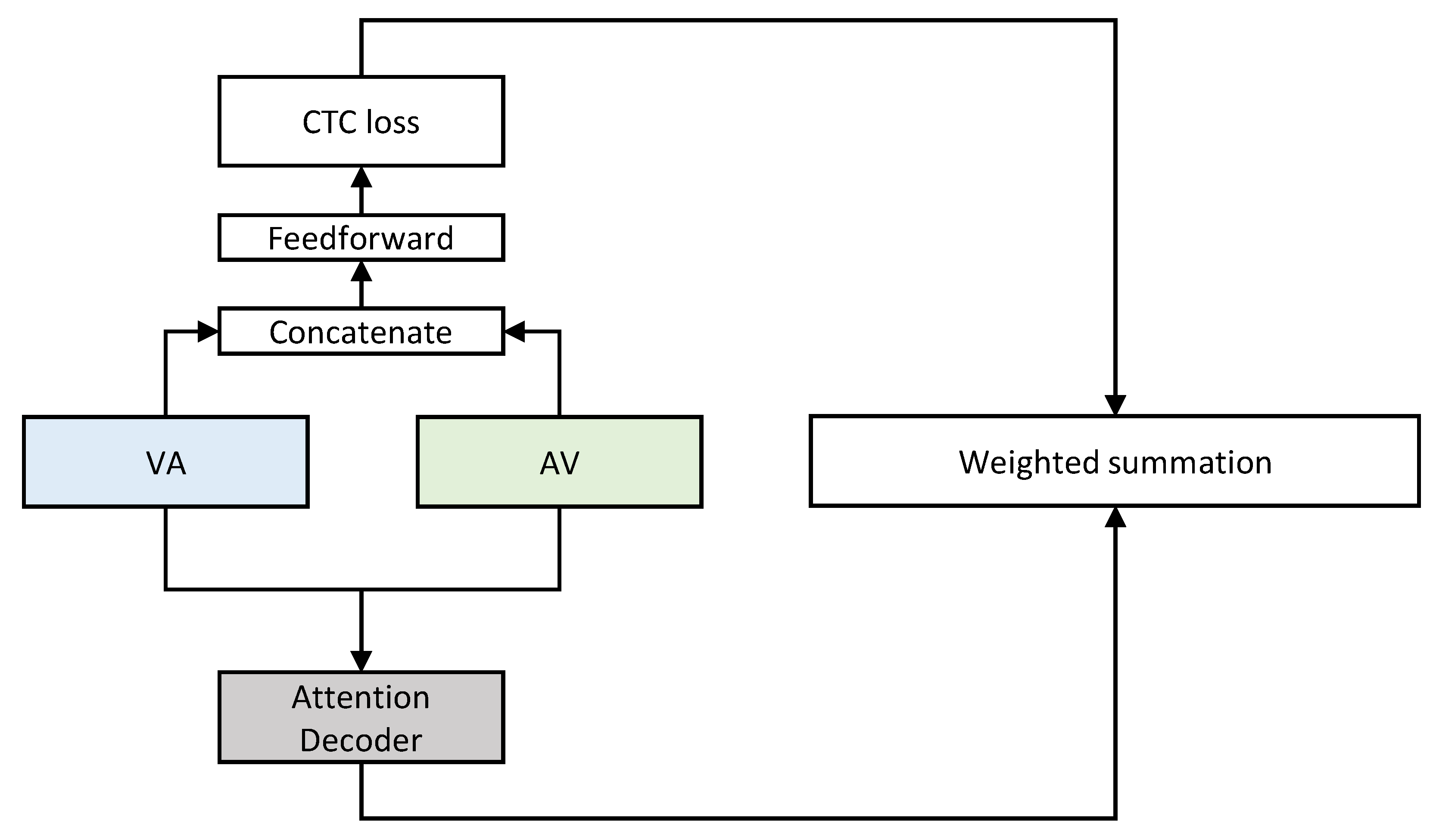
3.2.3. DCM Attention

The AV align model provided improved performance by fusing two modalities with attention in the encoder side instead of modality fusion in the decoder side [13]. However, when using audio as a query in the AV align model, attention weights may not be properly obtained in noisy environments. On the other hand, since video data is independent of acoustic noise, it may be important to make the role of video modality to a level of audio modality by fully exploiting input audio and visual information in learning attentions. Therefore, using video as a query may be helpful to achieve noise robustness. To consider a video query for audio context in addition to an audio query for video context of the AV align model [13] and to apply them to the transformer model, our DCM attention model has two multi-head attention layers between the two modality encoders, as shown in Figure 3. The configuration of each multi-head attention layer used in the DCM attention model is the same as that in the multi-head attention used for the encoder and decoder. Using ${\mathbf{h}}^a$ and ${\mathbf{h}}^v$, DCM attention outputs, $\mathbf{AV}$ and $\mathbf{VA}$, can be expressed as

$$\begin{array}{cc}\hfill \mathbf{AV}& =\mathrm{Attention}\left({\mathbf{h}}^a,{\mathbf{h}}^v,{\mathbf{h}}^v\right),\\ \hfill \mathbf{VA}& =\mathrm{Attention}\left({\mathbf{h}}^v,{\mathbf{h}}^a,{\mathbf{h}}^a\right).\end{array}$$

(16)

3.2.4. Bi-Modal Self-Attention Decoder

We use an architecture similar to the seq2seq transformer (TM-seq2seq) model by Afouras et al. [20]. We use six decoder blocks. Each block has one multi-head self attention and two multi-head encoder–decoder attentions. Each encoder–decoder attention uses previous decoder outputs after the self attention as queries and DCM attention outputs as keys and values. Then, the two encoder–decoder attention outputs (${\mathbf{AV}}_c,{\mathbf{VA}}_c$), as shown in Figure 4, are concatenated channel-wise and fed to fusion layers for calculating attentional vector ${\tilde{s}}_i$ at decoder time step i, which is expressed as

$$\begin{array}{cc}\hfill {\tilde{s}}_i=& \mathrm{LayerNorm}(\mathrm{FusionLayer}\left([{\mathbf{AV}}_c,{\mathbf{VA}}_c]\right)+[{\mathbf{AV}}_c,{\mathbf{VA}}_c]),\end{array}$$

(17)

where $\mathrm{FusionLayer}$ denotes modality fusion layers composed of two fully connected layers, rectified linear units, and dropout as shown in Figure 4. Finally, like (8), the predictive character distribution is obtained from calculating the attentional vector ${\tilde{s}}_i$. Detailed hyper-parameters in the multi-head attentions and the feed-forward layers are identical to those in the encoder.

3.3. Training and Decoding with a Hybrid CTC/Attention Architecture

Similar to [19], a CTC loss is combined with an objective for our attention-based model to force a monotonic alignment required for speech recognition during training. The resulting loss function is a weighted sum of the CTC and attention objectives, which is computed as follows:

$$\mathcal{L}=\alpha log{p}_{\mathrm{ctc}}\left(\mathbf{y}\mathbf{x}\right)+(1-\alpha )log{p}_{\mathrm{att}}\left(\mathbf{y}\mathbf{x}\right),$$

(18)

where $\mathbf{y}=(y_1,\cdots ,y_I)$, $\mathbf{x}$, and $\alpha$ denote a decoded output character sequence, input feature sequences from both modalities, and a relative weight for the loss function, respectively. A decoded output character may include an extra end-of-sentence label. In the training phase, a ground truth character sequence is used as a target label, and the detailed method is shown in Algorithm 1.

To calculate the CTC loss, we need to fuse the audio and video encoder results as shown in Figure 5. Therefore, the video encoder output is upsampled to have a sequence with the same length as the audio encoder output. After that, the two encoder outputs are concatenated channel-wise and fed to a feed-forward layer.

Algorithm 1: Hybrid CTC/attention training

In the decoding phase, we use a joint CTC/attention approach. We calculate a joint score based on CTC and attention decoder probabilities for decoded output character sequences. A hypothesis character output sequence $\widehat{\mathbf{y}}$ is computed as

$$\widehat{\mathbf{y}}=\underset{\mathbf{y}}{arg\; max}\{\lambda log{p}_{\mathrm{ctc}}\left(\mathbf{y}\mathbf{x}\right)+(1-\lambda )log{p}_{\mathrm{att}}\left(\mathbf{y}\mathbf{x}\right)\},$$

(19)

where $\lambda$ is a relative weight in the decoding phase. $\alpha$ and $\lambda$ are respectively set to 0.2 and 0.1 that are the same as in [19].

4. Experimental Results and Discussions

In this section, we describe our experimental setup and training strategies. Our proposed model was evaluated and compared with others.

4.1. Datasets

We used LRS datasets, the largest existing public AVSR datasets [20]. Unfortunately, due to the license restriction of MV-LRS [40], we used only LRS2-BBC and LRS3-TED datasets for training, validation, and testing. To improve robustness in noisy environments, we simulated noisy reverberant signals with the signal-to-noise ratios (SNRs) of $-5$ to 20 dB and the reverberation time (${\mathrm{RT}}_{60}$) of 0.4 s by adding babble noise samples acquired at cafeterias and restaurants and imposing reverberation generated by the image method [41] to clean speech signals from the datasets. The added noise samples were different for training and testing.

4.2. Evaluation Measure

The performance of the models was evaluated by the word error rate (WER) defined as

$$\mathrm{WER}=\frac{S+D+I}{N},$$

(20)

where $S,D,$ and I are the counts of substitutions, deletions, and insertions between reference and hypothesis word sequences, respectively, and N denotes the number of words for the reference.

4.3. Training Strategies

We trained in an order of clean short sentences, clean sentences, and clean/noisy reverberant sentences. The detailed data in the order are as follows:

• Clean short sentences with three or four words in the pre-train set.
• Clean sentences in the pre-train and train-val sets.
• Clean and noisy reverberant sentences (as described in Section 4.1) in the train-val set.
• Clean and noisy reverberant sentences in the train-val set of either LRS2-BBC or LRS3-TED dataset for fine tuning on either dataset.

Our implementation was based on the PyTorch library [42] and the fairseq toolkit [43]. We used the Adadelta optimizer [44] with default parameters. The learning rate started with ${10}^{-1}$ and decreased by half to ${10}^{-5}$ depending on the validation error plateaus. The dropout was performed with $p=0.15$. The implementation code of our proposed model is available at https://github.com/LeeYongHyeok/DCM_vgg_transformer.

4.4. Attention Visualization

Figure 6 shows the attention weight maps between audio and video encoders using audio or video features as queries in our proposed model (TM-DCM) for clean and noisy reverberant data. The weights were computed by averaging over all the cross-modality attention heads. The weight map of the audio query cross-modality attention for noisy reverberant data was more noisy than that for clean data because noisy reverberant data could not provide clear clues than clean data, which might result in performance degradation by speech contamination. However, the video query cross-modality attention produced very clean weight maps even with noisy reverberant audio data as keys and values.

In Figure 7, we display the encoder–decoder attention weight maps using previous decoder outputs after the self attention as queries and DCM attention outputs as keys and values for the cross-entropy and hybrid CTC/attention losses. The hybrid architecture made the maps, especially between audio encoders and decoders, more clean by forcing monotonic alignments even with noisy reverberant data.

4.5. WER Results

Table 1. Word error rates (WERs) (%) for the TM-seq2seq, TM-av_align, and TM-DCM on the LRS2-BBC and LRS3-TED datasets. The boldface WERs denote the best performance in each condition. Abbreviation to understand the table: A, audio-only modality; V, video-only modality; AV, audio–visual modalities; CE, cross-entropy loss only; H, hybrid CTC/attention loss; As a result that the video-only modality case (V) does not use the audio modality, we have a constant WER for each dataset on the TM-seq2seq using the video-only modality in the first two rows.

Model	Modality	Objective	#Params	Dataset		Clean	Noisy Reverberant						Avg.
				LRS2-BBC	LRS3-TED		SNR (dB)
							20	15	10	5	0	$-5$
TM-seq2seq	V	CE	54.2 M	✓		59.7
					✓	67.3
TM-seq2seq	A	CE	47.3 M	✓		9.8	21.7	23.3	25.7	33.7	47.6	68.9	33.0
					✓	10.1	21.4	23.5	26.1	33.8	48.1	69.6	33.2
TM-seq2seq	AV	CE	84.6 M	✓		10.5	19.7	19.8	23.0	25.1	34.0	43.7	25.1
					✓	10.8	20.0	20.2	23.5	27.6	36.4	51.3	27.1
TM-av_align	AV	CE	76.2 M	✓		11.5	18.8	19.3	22.6	25.0	31.2	43.4	22.6
					✓	11.7	18.1	18.9	21.8	25.8	34.1	47.1	25.4
TM-DCM	AV	CE	86.7 M	✓		8.7	17.3	17.5	19.2	22.0	29.2	41.2	22.2
					✓	9.0	17.8	18.0	19.8	22.9	31.5	45.8	23.5
TM-DCM	AV	H	86.7 M	✓		8.6	16.8	16.9	18.8	22.0	28.9	40.7	21.8
					✓	8.8	17.1	17.3	19.2	22.2	30.9	43.6	22.7

summarizes the word error rates (WERs) for our proposed model (TM-DCM), the TM-seq2seq, and the AV align implemented on the transformer model (TM-av_align). The TM-seq2seq model was implemented using modality-independent encoder–decoder attention as described in [20]. For fair comparison, the TM-av_align model was implemented by applying the cross-modal alignment structure in [13] to the TM-seq2seq model used as the common baseline model and performed modality fusion with attention using audio as a query on the encoder side while our proposed model added the DCM to the baseline model. In the modality column, ‘A’, ‘V’, and ‘AV’ denote that audio-only, video-only, and audio–visual modalities were used, respectively. In the objective column, ‘CE’ and ‘H’ mean the objective functions based on the cross-entropy only and the hybrid CTC/attention loss, respectively. In addition, the numbers of parameters in the used models are presented, and our model requiring two additional attentions for DCM has 2.5% more parameters than the TM-seq2seq.

Table 2. Architectural differences in cross-modality attentions between the TM-seq2seq, TM-av_align, and TM-DCM.

Model	TM-seq2seq	TM-av_align	TM-DCM
Modality attention	None	Audio–Video	Audio–Video and Video–Audio
(Query-Key/Value)

describes architectural differences in cross-modality attentions between the three models since the cross-modality attention architectures are mainly different with audio–visual modalities.

Regardless of the used methods, the WERs increased as the SNR decreased. The relatively significant differences in WERs between clean and 20-dB noisy reverberant data were possibly caused by the reverberation to simulate realistic situations. In the case of using the cross-entropy only as a loss function, our model consistently provided better recognition performance than the TM-seq2seq and the TM-av_align regardless of the input SNRs. In particular, the WER of our model averaged over the two datasets achieved a relative improvement of about 16.9% for clean data compared to that of the TM-seq2seq (much larger than the parameter growth rate) whereas the TM-av_align showed comparable or slightly deteriorated performance than the TM-seq2seq. These results were because our model could effectively fuse the modality information by the video query cross-modality attention in addition to the audio query cross-modality attention similar to the AV align model. As shown in Figure 6, clean weight maps of the video query cross-modality attention in our model were helpful for recognition of noisy reverberant audio data as well as clean data.

Adding the CTC loss in the hybrid CTC/attention architecture to assess the contribution of the CTC loss further improved the recognition performance, which demonstrated that monotonic alignments were very useful for speech recognition. These results were consistent with more clean encoder–decoder attention weight maps. Above all, our model using the DCM attention and the hybrid CTC/attention loss achieved the WER of 8.7% averaged over the two datasets for clean data with consistent better performance for all the experimented conditions than the others.

4.6. Decoding Examples

Table 3. Some decoding results for 0-dB-SNR noisy reverberant data. The boldface words denote wrong prediction. Abbreviation to understand the table: A, audio-only modality; V, video-only modality; AV, audio–visual modalities; CE, cross-entropy loss only; H, hybrid CTC/attention loss.

Models	Modality	Objective	Transcription
Ground truth			and it’s even rarer to find one that hasn’t been dug into by antiquarans
TM-seq2seq	V	CE	and it’s even rarer to find one that hasn’t bin diagnosed by asking quarries
TM-seq2seq	A	CE	and it’s equal rare two find one that hasn’t been dug into by anti crayons
TM-seq2seq	AV	CE	and it’s even rarer to find one that hasn’t been dug into by antique areas
TM-av_align	AV	CE	and it’s even rarer to find one that hasn’t been dug into by antiquarists
TM-DCM	AV	CE	and it’s even rarer to find one that hasn’t been dug into by antiquate risks
TM-DCM	AV	H	and it’s even rarer to find one that hasn’t been dug into by antiquarans
Ground truth			home to an animal that is right at the top of the food chain
TM-seq2seq	V	CE	home to an animal has raised in some of the future in
TM-seq2seq	A	CE	home to an animal bad is rights into top off a food chain
TM-seq2seq	AV	CE	home to an animal that is right at the top over food chain
TM-av_align	AV	CE	home to an animal that is right at the top of a food chain
TM-DCM	AV	CE	home to an animal that is right at the top of the food chain
TM-DCM	AV	H	home to an animal that is right at the top of the food chain
Ground truth			and would eventually marry her after his wife
TM-seq2seq	V	CE	and would eventually the most american hundreds of
TM-seq2seq	A	CE	and would eventually marry him got the his wife
TM-seq2seq	AV	CE	and would emit actually marry her after his wife
TM-av_align	AV	CE	and would emitting her after his wife
TM-DCM	AV	CE	and would eventually marry her after his wife
TM-DCM	AV	H	and would eventually marry her after his wife

shows some decoding results for 0-dB-SNR noisy reverberant data. Using video-only modality provided inferior performance to the others due to its inherent ambiguity in visual speech recognition. Using audio-only modality with speech contamination, it was difficult to recognize similar pronunciations such as “to”-“two”, “that”-“bad”, “of the”-“off a”. The methods using both the modalities mitigated the disadvantages for the uni-modalities by fusing audio and video information. In particular, our model that achieved superior performance to the others predicted correct words successfully except a very unusual word “antiquarans”.

4.7. Decoding on Sentences of Various Lengths

In Figure 8, we summarize the WERs according to the numbers of words in sentences for clean and noisy reverberant data. For both the data, our models achieved better recognition performance than the others in most cases. All the experimented models obtained poor performance for short sentences of three and four words because appropriate contexts could not be extracted in these sentences.

4.8. Decoding on Out-of-Sync Data

Figure 9 displays the WERs on out-of-sync data for clean and noisy reverberant data. Since audio and video were synchronized in the datasets, we synthetically shifted the video frames to get out-of-sync data as in [20]. Although the transformer model with the CTC loss only showed worse performance than that with the cross-entropy loss in [20], our model with the hybrid CTC/attention loss provided comparable WERs with the cross-entropy loss. Even with the CTC loss, our model still had robustness against out-of-sync data because our model was based on independent encoder–decoder and cross-modality attention mechanisms. The results demonstrated that our model might use the hybrid CTC/attention loss to force monotonic alignments required for AVSR without concerning relative performance degradation for out-of-sync data.

4.9. Comparison with Simple Concatenation of Audio and Video Encoder Outputs

In order to show the effectiveness of DCM attention,

Table 4. WERs (%) for our model and decoding on simple concatenation of audio and video encoder outputs on the test sets of LRS2-BBC and LRS3-TED datasets. The boldface WERs denote the best performance in each condition. Abbreviation to understand the table: CE, cross-entropy loss only; H, hybrid CTC/attention loss.

Fusion Method			Concatenation	TM-DCM
Objective			CE	CE	H
Clean			9.6	8.8	8.7
Noisy reverberant	SNR (dB)	20	18.2	17.5	16.9
		15	18.9	17.7	17.0
		10	21.2	19.4	18.9
		5	25.2	22.3	22.1
		0	33.5	30.0	29.5
		$-5$	47.3	42.7	41.7
Avg.			24.8	22.6	22.1

compares the WERs of our model with those for decoding on simple concatenation of audio and video encoder outputs. For all the experimented SNRs, our model outperformed the model using simple concatenation of audio and video information, which demonstrated the effectiveness of DCM attention.

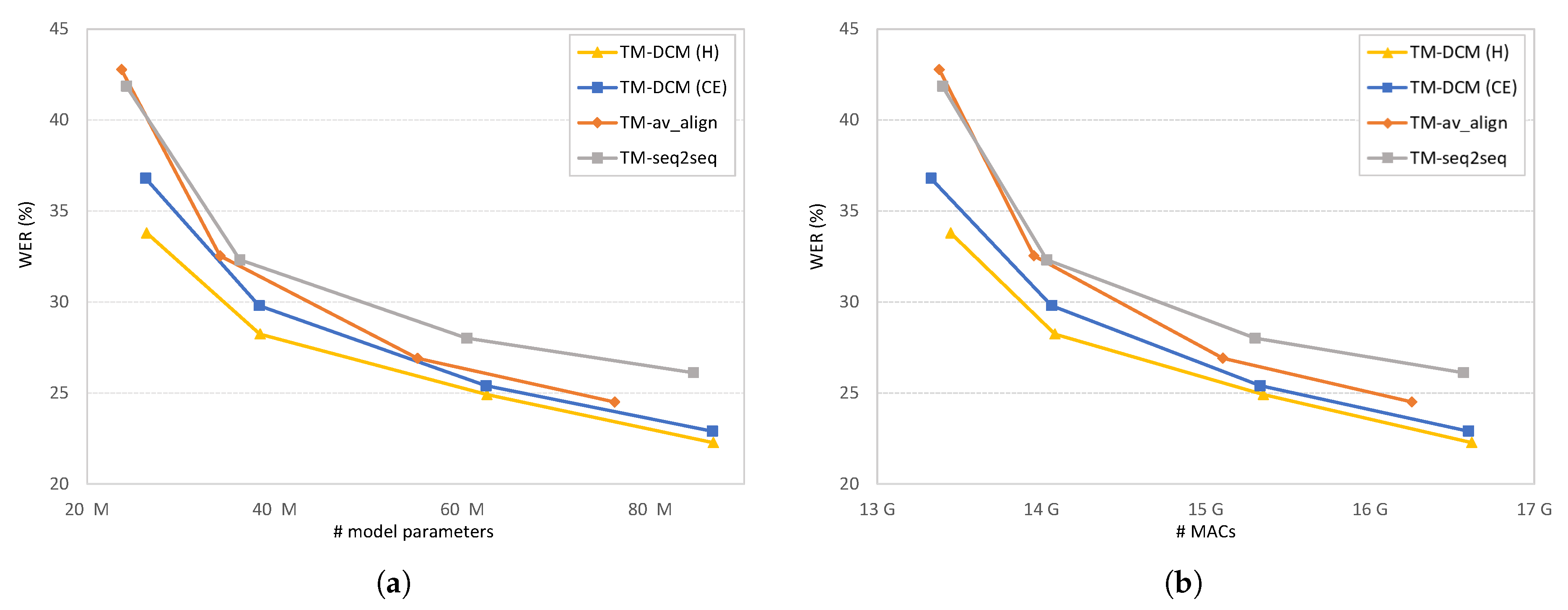
4.10. Model Parameter Sensitiveness and Run-Time Complexity

Figure 10 shows the WERs averaged over clean/noisy reverberant test data with all the experimented SNRs for various model sizes. For each model, we stacked encoders and decoders in various layers. Since the numbers of trainable model parameters and multiply-accumulate operations (MACs) are different for each model, Figure 10a,b display the WERs with the numbers of model parameters and MACs on the horizontal axis, respectively. The experimental results showed that our model yielded better recognition performance than the other compared models especially with smaller models, which indicated that our DCM structure and hybrid CTC/attention loss were efficient for fusion of audio and video.

5. Conclusions

In this paper, we proposed an AVSR model based on the transformer with the DCM attention and a hybrid CTC/attention architecture. We constructed the DCM attention for proper alignment information between audio and visual modality even with noisy reverberant audio data, and applied a hybrid CTC/attention structure to enhance monotonic alignments. In general, our model provided better recognition performance than the compared models based on the transformer, even for out-of-sync data, and the hybrid CTC/attention loss further improved the performance. In the future, we will focus on more efficient fusion strategy of audio and video information and extend to audio–visual speech recognition including a speech enhancement model.

References

1. Virtanen, T.; Singh, R.; Raj, B. (Eds.) Techniques for Noise Robustness in Automatic Speech Recognition; John Wiley & Sons, Ltd.: Hoboken, NJ, USA, 2012. [Google Scholar]
2. Wölfel, M.; McDonough, J. Distant Speech Recognition; John Wiley & Sons, Ltd.: Hoboken, NJ, USA, 2009. [Google Scholar]
3. Droppo, J.; Acero, A. Environmental Robustness. In Handbook of Speech Processing; Springer: Berlin, Germany, 2008. [Google Scholar]
4. Raj, B.; Parikh, V.; Stern, R.M. The effects of background music on speech recognition accuracy. In Proceedings of the IEEE International Conference on Acoustics, Speech, and Signal Processing (ICASSP), Munich, Germany, 21–24 April 1997; Volume 2, pp. 851–854. [Google Scholar]
5. Cho, J.W.; Park, J.H.; Chang, J.H.; Park, H.M. Bayesian feature enhancement using independent vector analysis and reverberation parameter re-estimation for noisy reverberant speech recognition. Comput. Speech Lang. 2017, 46, 496–516. [Google Scholar] [CrossRef]
6. Zhou, Z.; Zhao, G.; Hong, X.; Pietikäinen, M. A review of recent advances in visual speech decoding. Image Vis. Comput. 2014, 32, 590–605. [Google Scholar] [CrossRef]
7. Chung, J.S.; Senior, A.; Vinyals, O.; Zisserman, A. Lip reading sentences in the wild. In Proceedings of the IEEE Computer Vision and Pattern Recognition (CVPR), Honolulu, HI, USA, 21–26 July 2017; pp. 3444–3453. [Google Scholar]
8. Dalal, N.; Triggs, B. Histograms of oriented gradients for human detection. In Proceedings of the IEEE Computer Vision and Pattern Recognition (CVPR), San Diego, CA, USA, 20–26 June 2005; Volume 1, pp. 886–893. [Google Scholar]
9. Ahonen, T.; Hadid, A.; Pietikainen, M. Face description with local binary patterns: Application to face recognition. IEEE Trans. Pattern Anal. Mach. Intell. (TPAMI) 2006, 28, 2037–2041. [Google Scholar] [CrossRef] [PubMed]
10. Lowe, D.G. Distinctive image features from scale-invariant keypoints. Int. J. Comput. Vis. 2004, 60, 91–110. [Google Scholar] [CrossRef]
11. Jang, D.W.; Kim, H.I.; Je, C.; Park, R.H.; Park, H.M. Lip Reading Using Committee Networks With Two Different Types of Concatenated Frame Images. IEEE Access 2019, 7, 90125–90131. [Google Scholar] [CrossRef]
12. Noda, K.; Yamaguchi, Y.; Nakadai, K.; Okuno, H.G.; Ogata, T. Audio-visual speech recognition using deep learning. Appl. Intell. 2015, 42, 722–737. [Google Scholar] [CrossRef] [Green Version]
13. Sterpu, G.; Saam, C.; Harte, N. Attention-based audio-visual fusion for robust automatic speech recognition. In Proceedings of the International Conference on Multimodal Interaction, Boulder, CO, USA, 16–20 October 2018; Volume 5, pp. 111–115. [Google Scholar]
14. Petridis, S.; Stafylakis, T.; Ma, P.; Cai, F.; Tzimiropoulos, G.; Pantic, M. End-to-end audiovisual speech recognition. In Proceedings of the IEEE International Conference on Acoustics, Speech, and Signal Processing (ICASSP), Calgary, AB, Canada, 15–20 April 2018; pp. 6548–6552. [Google Scholar]
15. Shillingford, B.; Assael, Y.; Hoffman, M.W.; Paine, T.; Hughes, C.; Prabhu, U.; Liao, H.; Sak, H.; Rao, K.; Bennett, L.; et al. Large-Scale Visual Speech Recognition. In Interspeech; 2019; pp. 4135–4139. Available online: https://arxiv.org/pdf/1807.05162.pdf (accessed on 20 September 2020).
16. Zhou, P.; Yang, W.; Chen, W.; Wang, Y.; Jia, J. Modality attention for end-to-end audio-visual speech recognition. In Proceedings of the IEEE International Conference on Acoustics, Speech, and Signal Processing (ICASSP), Brighton, UK, 12–17 May 2019; pp. 6565–6569. [Google Scholar]
17. Bahdanau, D.; Cho, K.; Bengio, Y. Neural Machine Translation by Jointly Learning to Align and Translate. In Proceedings of the International Conference on Learning Representations (ICLR), San Diego, CA, USA, 7–9 May 2015. [Google Scholar]
18. Zeyer, A.; Bahar, P.; Irie, K.; Schlüter, R.; Ney, H. A comparison of transformer and LSTM encoder decoder models for ASR. In Proceedings of the IEEE Automatic Speech Recognition and Understanding (ASRU) Workshop, Sentosa, Singapore, 14–18 December 2019; pp. 8–15. [Google Scholar]
19. Petridis, S.; Stafylakis, T.; Ma, P.; Tzimiropoulos, G.; Pantic, M. Audio-visual speech recognition with a hybrid CTC/attention architecture. In Proceedings of the IEEE Spoken Language Technology Workshop (SLT), Athens, Greece, 18–21 December 2018; pp. 513–520. [Google Scholar]
20. Afouras, T.; Chung, J.S.; Senior, A.; Vinyals, O.; Zisserman, A. Deep audio-visual speech recognition. IEEE Trans. Pattern Anal. Mach. Intell. (TPAMI) 2018. [Google Scholar] [CrossRef] [PubMed] [Green Version]
21. Mroueh, Y.; Marcheret, E.; Goel, V. Deep multimodal learning for Audio-Visual Speech Recognition. In Proceedings of the IEEE International Conference on Acoustics, Speech and Signal Processing (ICASSP), South Brisbane, Australia, 19–24 April 2015; pp. 2130–2134. [Google Scholar]
22. Tamura, S.; Ninomiya, H.; Kitaoka, N.; Osuga, S.; Iribe, Y.; Takeda, K.; Hayamizu, S. Audio-visual speech recognition using deep bottleneck features and high-performance lipreading. In Proceedings of the Asia-Pacific Signal and Information Processing Association Annual Summit and Conference (APSIPA), Hong Kong, China, 16–19 December 2015; pp. 575–582. [Google Scholar]
23. Galatas, G.; Potamianos, G.; Makedon, F. Audio-visual speech recognition incorporating facial depth information captured by the Kinect. In Proceedings of the 20th European Signal Processing Conference (EUSIPCO), Bucharest, Romania, 27–31 August 2012; pp. 2714–2717. [Google Scholar]
24. Vaswani, A.; Shazeer, N.; Parmar, N.; Uszkoreit, J.; Jones, L.; Gomez, A.N.; Kaiser, Ł.; Polosukhin, I. Attention is all you need. In Proceedings of the Advances in Neural Information Processing Systems (NeurIPS), Long Beach, CA, USA, 4–9 December 2017; pp. 5998–6008. [Google Scholar]
25. Wang, Y.; Mohamed, A.; Le, D.; Liu, C.; Xiao, A.; Mahadeokar, J.; Huang, H.; Tjandra, A.; Zhang, X.; Zhang, F.; et al. Transformer-based acoustic modeling for hybrid speech recognition. arXiv 2019, arXiv:1910.09799. [Google Scholar]
26. Yeh, C.F.; Mahadeokar, J.; Kalgaonkar, K.; Wang, Y.; Le, D.; Jain, M.; Schubert, K.; Fuegen, C.; Seltzer, M.L. Transformer-Transducer: End-to-End Speech Recognition with Self-Attention. arXiv 2019, arXiv:1910.12977. [Google Scholar]
27. Paraskevopoulos, G.; Parthasarathy, S.; Khare, A.; Sundaram, S. Multimodal and Multiresolution Speech Recognition with Transformers. In Proceedings of the 58th Annual Meeting of the Association for Computational Linguistics, Seattle, DC, USA, 6–8 July 2020; pp. 2381–2387. [Google Scholar]
28. Sterpu, G.; Saam, C.; Harte, N. Should we hard-code the recurrence concept or learn it instead? Exploring the Transformer architecture for Audio-Visual Speech Recognition. arXiv 2020, arXiv:2005.09297. [Google Scholar]
29. Boes, W.; Van hamme, H. Audiovisual Transformer Architectures for Large-Scale Classification and Synchronization of Weakly Labeled Audio Events. In Proceedings of the 27th ACM International Conference on Multimedia, Nice, France, 21–25 October 2019; pp. 1961–1969. [Google Scholar]
30. Li, Z.; Li, Z.; Zhang, J.; Feng, Y.; Niu, C.; Zhou, J. Bridging Text and Video: A Universal Multimodal Transformer for Video-Audio Scene-Aware Dialog. arXiv 2020, arXiv:2002.00163. [Google Scholar]
31. Le, H.; Sahoo, D.; Chen, N.; Hoi, S. Multimodal Transformer Networks for End-to-End Video-Grounded Dialogue Systems. In Proceedings of the 57th Annual Meeting of the Association for Computational Linguistics, Florence, Italy, 28 July–2 August 2019; Volume 2, pp. 5612–5623. [Google Scholar]
32. Tsai, Y.H.H.; Bai, S.; Liang, P.P.; Kolter, J.Z.; Morency, L.P.; Salakhutdinov, R. Multimodal Transformer for Unaligned Multimodal Language Sequences. In Proceedings of the 57th Annual Meeting of the Association for Computational Linguistics, Florence, Italy, 28 July–2 August 2019; Volume 2019, pp. 6558–6569. [Google Scholar]
33. Chan, W.; Jaitly, N.; Le, Q.; Vinyals, O. Listen, attend and spell: A neural network for large vocabulary conversational speech recognition. In Proceedings of the IEEE International Conference on Acoustics, Speech, and Signal Processing (ICASSP), Shanghai, China, 20–25 March 2016; pp. 4960–4964. [Google Scholar]
34. Luong, M.T.; Pham, H.; Manning, C.D. Effective Approaches to Attention-based Neural Machine Translation. In Proceedings of the Conference on Empirical Methods in Natural Language Processing (EMNLP), Lisbon, Portugal, 17–21 September 2015; pp. 1412–1421. [Google Scholar]
35. Watanabe, S.; Hori, T.; Kim, S.; Hershey, J.R.; Hayashi, T. Hybrid CTC/attention architecture for end-to-end speech recognition. IEEE J. Sel. Top. Signal Process. 2017, 11, 1240–1253. [Google Scholar] [CrossRef]
36. Xu, K.; Li, D.; Cassimatis, N.; Wang, X. LCANet: End-to-end lipreading with cascaded attention-CTC. In Proceedings of the 13th IEEE International Conference on Automatic Face & Gesture Recognition (FG 2018), Xi’an, China, 15–19 May 2018; pp. 548–555. [Google Scholar]
37. Mohamed, A.; Okhonko, D.; Zettlemoyer, L. Transformers with convolutional context for ASR. arXiv 2019, arXiv:1904.11660. [Google Scholar]
38. Chung, J.S.; Zisserman, A. Out of time: Automated lip sync in the wild. In Asian Conference on Computer Vision (ACCV); Springer: Berlin, Germany, 2016; pp. 251–263. [Google Scholar]
39. Chatfield, K.; Simonyan, K.; Vedaldi, A.; Zisserman, A. Return of the devil in the details: Delving deep into convolutional nets. In Proceedings of the British Machine Vision Conference (BMVC), Nottingham, UK, 1–5 September 2014. [Google Scholar]
40. Chung, J.S.; Zisserman, A. Lip Reading in Profile. In Proceedings of the British Machine Vision Conference (BMVC), London, UK, 4–7 September 2017. [Google Scholar]
41. Allen, J.B.; Berkley, D.A. Image method for efficiently simulating small-room acoustics. J. Acoust. Soc. Am. 1979, 65, 943–950. [Google Scholar] [CrossRef]
42. Paszke, A.; Gross, S.; Chintala, S.; Chanan, G.; Yang, E.; DeVito, Z.; Lin, Z.; Desmaison, A.; Antiga, L.; Lerer, A. Automatic differentiation in PyTorch. In Proceedings of the Neural Information Processing Systems (NeurIPS) Workshop, Long Beach, CA, USA, 4–9 December 2017. [Google Scholar]
43. Ott, M.; Edunov, S.; Baevski, A.; Fan, A.; Gross, S.; Ng, N.; Grangier, D.; Auli, M. fairseq: A Fast, Extensible Toolkit for Sequence Modeling. In Proceedings of the Conference of the North American Chapter of the Association for Computational Linguistics (Demonstrations), Minneapolis, MN, USA, 2–7 June 2019; pp. 48–53. [Google Scholar]
44. Zeiler, M.D. ADADELTA: An Adaptive Learning Rate Method. arXiv 2012, arXiv:1212.5701. [Google Scholar]
Figure 1. An overview of our proposed audio–visual speech recognition (AVSR) architecture. It consists of four modules: encoders, dual cross-modality (DCM) attentions, an attention decoder, and a connectionist-temporal-classification (CTC) block. The encoders receive each modality and compress their information. DCM attentions are calculated by using different modalities for the queries and the keys. Finally, character probabilities are calculated by using both the attention decoder and the CTC block.
Applsci 10 07263 g001
Figure 2. Encoder structures. Each structure generates audio or video features using a multi-head self attention followed by two feed-forward layers (FC 1 and FC 2). The number of encoder blocks, N, is six in these structures. (a) Video encoder; (b) audio encoder.
Applsci 10 07263 g002
Figure 3. DCM attention architecture. Either audio or video encoder output as a query Q is fused with the other modality as a key K and a value V in a multi-head attention. AV and VA denote the audio query encoder and video query encoder outputs, respectively.
Applsci 10 07263 g003
Figure 4. Decoder structure. Similar to the transformer sequence-to-sequence (TM-seq2seq) model, the transformer with DCM attention (TM-DCM) model receives the audio query encoder output (AV) and video query encoder output (VA) and returns character probabilities. Context vectors (AVc and VAc) computed by multi-head encoder–decoder attentions are concatenated channel-wise and fed to feed-forward layers.
Applsci 10 07263 g004
Figure 5. Procedure to compute the loss function for the TM-DCM model. The TM-DCM model is trained by using the hybrid CTC/attention architecture to force monotonic alignments required for speech recognition.
Applsci 10 07263 g005
Figure 6. DCM attention weight maps between audio and video encoders using audio or video features as queries in the TM-DCM for clean and noisy reverberant data. The used clean utterance was “PSlBlZ3hqKc/00011.mp4” in the test set of the LRS3-TED dataset, whose character label was “that is the real world and unless we find a way to globalize democracy or”. The input SNR for noisy reverberant data was 0 dB. The weights were computed by averaging over all the cross-modality attention heads. The weight maps for (a) clean audio query and video key/value; (b) noisy reverberant audio query and video key/value; (c) video query and clean audio key/value; and (d) video query and noisy reverberant audio key/value.
Applsci 10 07263 g006
Figure 7. Encoder–decoder attention weight maps using the DCM attention outputs as keys and values in the TM-DCM for the cross-entropy and hybrid CTC/attention losses. The weight maps were displayed for both clean and noisy reverberant data, and the used clean and noisy reverberant data were the same as in Figure 6. The weights were computed by averaging over all the encoder–decoder attention heads at all decoder layers. The weight maps for (ad) the cross-entropy loss and (eh) the hybrid CTC/attention loss; the weight maps between (a,e) audio encoders and decoders using clean audio input; (b,f) audio encoders and decoders using noisy reverberant audio input; (c,g) video encoders and decoders using clean audio input; and (d,h) video encoders and decoders using noisy reverberant audio input.
Applsci 10 07263 g007
Figure 8. WERs according to the numbers of words in sentences for the models using audio–visual modality on the test sets of LRS2-BBC and LRS3-TED datasets with (a) clean and (b) noisy reverberant audio data.
Applsci 10 07263 g008
Figure 9. WERs on out-of-sync data for the models using audio–visual modality on the test sets of LRS2-BBC and LRS3-TED datasets with (a) clean and (b) noisy reverberant audio data. The video frames were shifted by the numbers of frames on the horizontal axes with audio data fixed. The positive offset meant that the audio preceded the video, and the negative offset meant vice versa.
Applsci 10 07263 g009
Figure 10. WERs for various model sizes with the numbers of (a) trainable model parameters and (b) multiply-accumulate operations (MACs). The data used to measure the MACs were “PSlBlZ3hqKc/00011.mp4” in the test set of the LRS3-TED dataset.
Applsci 10 07263 g010