Learn and Tell: Learning Priors for Image Caption Generation

Abstract

In this work, we propose a novel priors-based attention neural network (PANN) for image captioning, which aims at incorporating two kinds of priors, i.e., the probabilities being mentioned for local region proposals (PBM priors) and part-of-speech clues for caption words (POS priors), into a visual information extraction process at each word prediction. This work was inspired by the intuitions that region proposals have different inherent probabilities for image captioning, and that the POS clues bridge the word class (part-of-speech tag) with the categories of visual features. We propose new methods to extract these two priors, in which the PBM priors are obtained by computing the similarities between the caption feature vector and local feature vectors, while the POS priors are predicated at each step of word generation by taking the hidden state of the decoder as input. After that, these two kinds of priors are further incorporated into the PANN module of the decoder to help the decoder extract more accurate visual information for the current word generation. In our experiments, we qualitatively analyzed the proposed approach and quantitatively evaluated several captioning schemes with our PANN on the MS-COCO dataset. Experimental results demonstrate that our proposed method could achieve better performance as well as the effectiveness of the proposed network for image captioning.

1. Introduction

The task of image caption aims at automatically giving a natural language description for an input image by using pre-designed algorithms operated on a computer [1,2], and this research lies at the intersection of two currently prevalent research fields, i.e., Computer Vision (CV) and Natural Language Process (NLP). These technologies have wide applications in our daily life, such as giving descriptive captions for retrieval and image indexing, giving robots stronger man–machine communication abilities, automatic video security monitoring, and helping people with visual impairments by translating visual signals into information that could be communicated through text-to-speech technology. Usually, caption models consist of two main parts, i.e., a encoder and a decoder, in which the encoder employs convolutional neural networks (CNNs) to extract visual features as image representation, and the decoder usually adopts a recurrent neural network (RNN) [1,3,4,5,6] or an attention-based neural network (such as transformer networks) [7,8,9,10,11] to decode visual features into flexible length sequences.

Recently, caption models tend to choose structural representation, i.e., Scene Graph, for input image features because of its advantage of being able to carry more detailed information. This is also inspired by the achievements [12,13,14] made in the field of CV. In this way, it is possible to give a caption with more image details that could be utilized for some specific design, for example, for caption diversity. The Scene Graph consists of three kinds of heterogeneous image visual feature sets (the object feature set, attribute feature set, and relation feature set), which are included as nodes, with the connections of each node pair considered edges. However, it is a challenge to extract corresponding visual information at each time step of word generation from various region proposals and heterogeneous features. This is partly caused by the difference between the tasks of object detection and image captioning. The authors of [15] proposed a method to incorporate three kinds of features into a single feature vector for each region proposal according to the existing connections in the graph so as to reduce the complexity, but some details may be lost in this method. In various studies [9,16,17,18], each kind of visual feature type and region proposal was treated equally, and an attention mechanism was applied to extract visual information. However, all of the above-mentioned works tried to compose their query vector in their attention module based on the hidden state of the decoder or the previous words while ignoring the PBM and POS priors’ impact for captioning, which could be used as a guide for visual information extraction.

In order to leverage the above-mentioned issue, the goal of this work is to utilize the probabilities being mentioned for region proposals (PBM priors) and part-of-speech of caption words (POS priors) in the attention module, to help the decoder more correctly focus on relevant region proposals and corresponding visual feature sets. The reasons that these two types of priors are helpful could be summarized as follows: (1) the intrinsic PBM priors could provide external guidance for the language module so that the decoder could better attend to these critical proposals with a lower chance of being misled. This inherent characteristic hints that areas with a high PBM would have a higher chance of being attended and mentioned, while the chance of the rest is relatively much lower. (2) The POS priors are investigated to explore the relationship between the word class and the feature class, i.e., a word with different POS tags could be directly derived from a corresponding feature set. For example, the object words referring to the objects mentioned in the caption, such as “cat” or “car”, could be obtained from the object visual feature set; the attribute words, such as “red” or “colorful”, could be obtained from the attribute visual feature set; and the relation words, such as “standing” or “walking”, could be obtained from the relation visual set. We take Figure 1 as an example to illustrate our intuition. There are several bounding boxes on the image, which indicate the local region of corresponding local visual features and are presented in different colors. When the decoder tries to generate the caption word “soccer”, our proposed POS module would first compute its part-of-speech distribution; this prior could pass the message that the next word is with high probability a noun to the decoder, and thus the attention module should put more attention on the object regions (features) rather than attribute and relation regions.

In our work, we propose a novel priors-based attention neural network (PANN) to incorporate the PBM priors and POS priors in the decoder. The whole work could be divided into two stages, i.e., the encoding stage and the decoding stage. In the encoding stage, the PBM priors for each region proposal are obtained according to the similarities between the local feature vectors and caption vector, in which the latter is extracted through the auxiliary multi-class multi-label task, while in the decoding stage, the POS priors of caption words are first predicated by taking the hidden state of the decoder as an input, and after that the PBM and POS priors are used in the weight calculation process in PANN. Finally, the assembled feature vector is output for the next work generation.

The study’s contributions lie in the following three aspects:

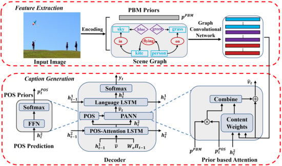
• We propose a novel prior-based attention neural network, in which two kinds of priors, i.e., the probability of being mentioned for region proposals (PBM priors) and part-of-speech of caption words (POS priors), are incorporated to help the decoder extract more accurate visual information at each step of word generation;
• We propose new methods to obtain the PBM and POS priors, in which we obtain PBM priors by computing the similarities between local feature vectors and the caption vector, while the POS priors are obtained by predicting the reduced POS tags so as to connect to the categories of visual features.
• We performed comprehensive evaluations on the image captioning benchmarks dataset MS-COCO, demonstrating that the proposed method outperforms several current state-of-the-art approaches in most metrics, and that the proposed priors-based attention neural network (PANN) could improve previous approaches.

The paper is structured as follows: we introduce related works in Section 2. After that, the extraction of the PBM priors, the POS priors, and the proposed PANN is discussed in Section 3. Then, implementation details and experiments are discussed in Section 4. Finally, conclusions are presented in Section 5.

2. Related Works

In this section, we will introduce related works that deal with three different aspects: attention mechanism, part-of-speech predication, and semantic clues.

Attention Mechanism. When the RCNN (regional convolutional neural network) features or scene graph are chosen as the input image representation, the attention mechanism is often adopted in the decoder to attend the related regions and further extract currently needed visual information for each word generation. These works could be sorted based on the attention network structure and the attention weight calculation method. (1) Single layer vs. multi-layer (see, for example, studies [3,4,19,20,21,21]) employs a single layer implement of an attention mechanism by taking the hidden state as the query vector to extract visual features at each step, while the studies [8,16,17,22,23] chose a multi-layer attention implementation in their decoder. (2) Involving extra clues in attention weights or not—for example, studies [11,24,25] obtained their attention weights only from previous attention calculations, while the authors of [18] combined geometry clues with previously calculated weights into final attention weights. However, all of these works only tried to make full use of intrinsic existing clues to calculate the attention weights but ignored the impact of the PBM and POS priors.

Part-of-Speech Prediction. The part-of-speech prediction task has been studied in recent decade, for example in the works [26,27,28,29,30]. In the text generation tasks, the word POS tag is predicted by the previous generated words and state of the decoder recursively. These works can be divided into two categories: (1) treated as a multi-task learning problem: for example, the authors of [26] treated POS tagging as an auxiliary task, i.e., predicting the POS tag for each word to be generated alongside the word generation, and the authors of [27] predicted the POS tag and name entity (NE) tag at the same time as word generation; (2) gate for external features: for example, the authors of [31,32] predicated the POS information for the word as a condition to determine whether the visual (external) feature is essential for current word generation. However, all of the above approaches did not utilize the POS priors to guide the heterogeneous visual feature assembly based on the intrinsic relationship between word class and feature categories.

Semantic Clues. Our extracted PBM priors are very similar to external semantic clues, which are usually obtained through an additional learning task or a pre-train model, such as in the the studies [3,33,34,35]. The main difference between our extracted PBM priors and the semantic clues lies in two aspects: (1) the PBM priors contain the probabilities of being mentioned for region proposals but no content information, while the semantic clues are usually considered as carrying intrinsic content information; (2) for the usage of semantic clues, the authors of [36] used a semantic embedding network layer to accept semantic clues as input and feed its output to the decoder, and the authors of [33] utilized tag vectors as semantic clues to guide the ensemble of parameters in the language model. However, in our work, the PBM priors are involved in the attention weight calculation process, indirectly helping the encoder to better focus on the correct areas in the visual information extraction process.

3. Priors-Based Attention Neural Network

3.1. Conventional Approach Revisited

The purpose of a captioning model is to give a natural language description, i.e., $\mathcal{S}=\{w_1,w_2,\cdots ,w_T\}$, for the input image $\mathcal{I}$. Recently, many models tend to adopt various kinds of visual features to enhance the performance of captioning, and these kinds of features are linked tightly and form a graph $\mathcal{G}=<\mathcal{N},\mathcal{E}>$, where $\mathcal{N}$ and $\mathcal{E}$ represent the nodes and edges, respectively. The nodes consist of the object nodes $\mathcal{O}$, attribute nodes $\mathcal{A}$, and relation nodes $\mathcal{R}$; this is formulated by $\mathcal{N}=\{\mathcal{O},\mathcal{A},\mathcal{R}\}$.

Usually, additional graph convolutional networks (GCNs) are applied on the obtained graph $\mathcal{G}$ to get more informative visual features sets ${\mathcal{G}}^{\prime }=\{{\mathcal{O}}^{\prime },{\mathcal{A}}^{\prime },{\mathcal{R}}^{\prime }\}$, and these networks are trained along with a captioning model, which is regarded as a message passing [37] process among nodes and edges. We present the implementation of three kinds of context-aware embeddings as follows:

Relaitonship Embedding. Given one relationship triple $<o_i,r_{ij},o_j>$ in $\mathcal{G}$, we have:

$$\widehat{r_{ij}}=g_r(e_{o_i},e_{r_{ij}},e_{o_j})$$

(1)

where the content of each relationship triplet is incorporated together, as shown in Figure 2a.

Attribute Embedding. Given an object node $o_i$ with its attribute $a_i$ in $\mathcal{G}$,

$$\widehat{a_i}=g_a((e_{o_i},e_{a_i})$$

(2)

where the context of this object and its attribute are incorporated, as shown in Figure 2b.

Object Embedding. An object $o_i$ could act as a “subject” or “object”, which means that the edge has different directions depending on its role; therefore, the $\widehat{o_i}$ can be calculated as:

$$\begin{array}{cc}\hfill \widehat{o_i}=\frac{1}{N_{r_i}}& [{\displaystyle \sum _{o_j\in sbj\left(o_i\right)}}{g}_s(e_{o_i},e_{o_j},e_{r_{ij}})+\hfill \\ \hfill & {\displaystyle \sum _{o_k\in obj\left(o_i\right)}}{g}_o(e_{o_k},e_{o_i},e_{r_{ki}})]\hfill \end{array}$$

(3)

where each node $o_j\in \mathrm{sbj}\left(o_i\right)$ acts as an “object” and $o_i$ acts as “subjects”, e.g., $\mathrm{sub}\left(o_2\right)=o_1$ in Figure 2c, and $N{r}_i=\left|\mathrm{sbj}\left(i\right)\right|+\left|\mathrm{obj}\left(i\right)\right|$ is the number of relationship triplets where $o_i$ appears.

In the decoding process, the attention mechanism is adopted to extract related information from the heterogeneous feature sets, which could be formulated as:

$$\widehat{v_t}=\mathrm{Attention}(\widehat{\mathcal{V}},h_{t-1})$$

(4)

where $h_{t-1}$ is the hidden state of the decoder at time step t, and $\widehat{\mathcal{V}}=[\widehat{\mathcal{O}},\widehat{\mathcal{A}},\widehat{\mathcal{R}}]$ are a stacked set by outputs of new object, attribute, and relation embeddings, respectively, obtained from the previously mentioned graph convolutional networks (GCNs).

Finally, the decoder takes the extracted feature vector $\widehat{v_t}$ along with the current hidden state to generate the word in the caption, which formulated as:

$$w_t=\mathrm{argmax}\left(\mathrm{FFN}\left(\mathrm{Decoder}(\widehat{v_t},h_{t-1},x_{t-1})\right)\right)$$

(5)

where $x_{t-1}$ is the embedding of the previous word as an external input, and $FFN$ is the two layers of a fully-connected feed-forward network.

3.2. Priors Extraction Process

PBM Priors Extraction. We adopted Faster-RCNN [13] to get local proposals and extract local visual feature vectors as well as their position in the image. As shown in Figure 3, we extract the caption vector to carry the caption information by predicting caption words in a multi-class multi-label classification task, and the PBM priors are further obtained by computing the cosine similarities between the encoded local feature vectors ($o_1,o_2,\dots ,o_{o_n}$) and caption feature vector c. Before the training (independently from the caption model training), we chose 220 unique caption object words from the caption vocabulary after removing singular and plural words. Let l be the ground truth caption feature vector, in which 1 or 0 in each dimension represent if the label appears or not in any of the ground truth captions. We also aligned the labels from the objection task with these 220 object labels, and trained the PBM module on the MS-COCO dataset. In this way, we define our objection function as:

$$\widehat{l_0}=Sigmoid\left(FF{N}_0\left(c\right)\right)$$

(6)

$$\widehat{l_i}=Softmax\left(FFN\left(o_i\right)\right),i\in 1,2,\dots ,o_{o_n}$$

(7)

$${\mathcal{L}}_{PBM}=\sum _i^n({\widehat{l}}_{i}log\left({\widehat{l}}_i\right)+(1-{\widehat{l}}_i)log(1-{\widehat{l}}_i)),i\in 0,1,2,\dots ,o_{o_n}$$

(8)

where c is the output of the inserted empty vector, i.e., the caption feature vector, and $o_i$, $i\in 1,2,\dots ,o_n$ is the encoded local feature, which would be used as an object feature in this work; $FF{N}_0$ and $FFN$ are two isolated fully-connected feed-forward networks. The ${\mathcal{L}}_{PBM}$ is the objective loss used to train the PBM module. The PBM priors for object regions are calculated as:

$$p_i^{PB{M}^o}=\frac{c·o_i}{\left|\right|c\left|\right|\ast \left|\right|o_i\left|\right|}$$

(9)

where $p_i^{PB{M}^o}$ is the PBM prior for the object region i.

After that, the attribute feature and relation feature were obtained by another independent training on the GNOME dataset using the method used in [12]. Note that the attribute region shares the same area as the object region, as shown in the left subfigure of Figure 1, and the relation (composed of the triplet <subject–predicate–object>) region is the union of the subject region and the object region. We define the PBM priors for the attribute region and relation region as:

$$p_i^{PB{M}^a}=p_i^{PB{M}^o}$$

(10)

$$p_{<i,j>}^{PB{M}^r}=\frac{p_i^{PB{M}^o}·p_j^{PB{M}^o}}{{\sum }_{(k,v)\in R}{p}_k^{PB{M}^o}\ast p_v^{PB{M}^o}}$$

(11)

where $p_i^{PB{M}^a}$ is the attribute region i, $p_{<i,j>}^{PB{M}^r}$ is the PBM prior for the relation r, R is the entire extracted relation triplet. For convenience, we denote $p^{PB{M}_i^{*}}$ as the PBM region i, if $iin\mathcal{A}$, $p^{PB{M}_i^{*}}=p^{PB{M}_i^a}$, and the same rule is applied to the attribute region and the relation region.

POS Priors Predication. As shown in Figure 4, we try to predict the part-of-speech at each step of the word prediction. In pre-processing, there are 25 POS tags in the tools of the NLTK, and we re-categorize these tags into four categories, i.e., the “object” class, “attribute” class, “relation” class, and “other” class, in order to build a connection with three kinds of visual features and the hidden state of the decoder. The object class corresponds to the objects in the caption; for instance, “car” and “bike” correspond to “blue” and “colorful” in the attribute class and “standing” and “in” in the relation class, whereas the “other” class contains most of virtual words, such as “the” and “of”. The POS label ground truth was prepared on the MS COCO training set, and the object function of this part is:

$$p_t^{POS}=Softmax\left(FFN\left(h_1^2\right)\right)$$

(12)

$${\mathcal{L}}_{POS}=-\frac{1}{K}\sum _{t=1}^K\sum _{j=1}^M{\overline{p}}_t^{PO{S}^{\left(j\right)}}log{p}_t^{PO{S}^{\left(j\right)}}+(1-{\overline{p}}_t^{PO{S}^{\left(j\right)}})log(1-p_t^{PO{S}^{\left(j\right)}})$$

(13)

where K is the length of the image caption, M is the dimension of the POS vector, and $FFN$ is the fully-connected feed-forward network. For convenience, we denote $p_t^{PO{S}^{*}}$ as the part-of-speech probability of tag *; for example, $p_t^{PO{S}^o}$ is the probability of the POS tag “object”.

3.3. Priors-Based Attention Neural Network

In this subsection, we will introduce our proposed priors-based attention neural network, in which two kinds of prior are involved in the visual feature extraction process at each time step of the decoding process. We will first describe the process of the computation process of the content weights $W^c$, in which the query vector is composed using the hidden state vector $h_t^2$ from POS-LSTM, shown at the bottom right of Figure 4. After that, we will incorporate the two types of priors obtained, i.e., $p^{PBM}$, and $p_t^{POS}$, into the final weights’ computation process.

Content Weight Computation. Suppose the input image $\mathcal{I}$ as presented using scene graph $\mathcal{G}$; we denote $V=[\mathcal{O},\mathcal{A},\mathcal{R}]$ as a visual feature set, i.e., the concatenation of three kinds of visual features. We chose the attention mechanism used in the work [7] as our bias. At the attention calculation process in each head, the query Q, key K, and value V will be calculated first using the following linear projections:

$$Q=h_t^2{W}_Q,K=V{W}_K,V=V{W}_V$$

(14)

where $W_Q,W_K,W_V$ are learned matrices for getting the query, key, and value, respectively. The content weights in each head are computed using dot products as follows:

$$w^c=\mathrm{Softmax}\left(\frac{Q{K}^T}{\sqrt{d_k}}\right)$$

(15)

where $d_k$ is a constant scaling factor; we set 64 as is the dimension of the key, query, and value matrix, as in the study [7].

Priors Fusion. As discussed before, the PBM priors contain the probabilities being mentioned for each region (including object region, attribute region, and relation region), and POS prior $p_t^{POS}$ could help the decoder focus on the visual features that have the most relevant feature category. We further fuse the extracted PBM priors and the POS priors with content weights according to their feature category and region position. We compute the element $w_i$ in final weights w as follows:

$$w_i=\lambda w_i^c+(1-\lambda )p_t^{PO{S}^{*}}{p}_i^{PB{M}^{*}}$$

(16)

where $\ast \in o,a,r$, for example, $\ast$ equals a, if the region i belongs to object region class, and same scheme applied to attribute regions, and relation regions. We choose addition operation here rather than the multiple operations, because the latter could extremely be affected by some minimal value and cause instability and performance drops.

After that, we will compute the output of each head as follows:

$$\mathrm{Head}(h_{t-1}^2,P^{PBM},p_t^{POS},V)=softmax\left(w\right)V$$

(17)

In the priors-based attention module, each head is calculated independently, and the final output is obtained by concatenating the output of all heads to one single vector and then multiplying it with a learned projection matrix $W_O$, i.e.,

$${\widehat{v}}_t=Concat({\mathrm{Head}}_1,\dots ,{\mathrm{Head}}_h)W_O$$

(18)

in which h is the number of heads in the attention module. Figure 5 illustrates the difference among priors based attention Figure 5a with standard transformer attention Figure 5b.

The ${\widehat{v}}_t$ would be fed into the language model to generate a caption word. We adopted the Up_Down [4] network structure as our decoder bias and replaced the original attention module with our proposed POS module and priors-based module, and the corresponding network structure is shown in Figure 4.

3.4. Training Objectives

First, we define the loss function for caption generation, given a target ground truth caption sequence $y_{1:T}^{*}$ and a captioning model with parameters $\theta$. We try to minimize the following cross-entropy loss:

$${\mathcal{L}}_{XE}\left(\theta \right)=-\sum _{t=1}^T\log \left(p_{\theta }\left(y_t^{*}\right|y_{1:t-1}^{*})\right)$$

(19)

For fair comparisons with the works trained using self-critical sequence training (SCST) [38], we also report the results optimized for CIDEr [39]. Initializing from the cross-entropy trained model, we seek to minimize the negative expected score:

$${\mathcal{L}}_R\left(\theta \right)=-E_{y_{1:T}{p}_{\theta }}\left[r\left(y_{1:T}\right)\right]$$

(20)

where r is the score function, i.e., CIDEr. The gradient of this loss can be approximated:

$${\nabla }_{\theta }{\mathcal{L}}_R\left(\theta \right)\approx -(r\left(y_{1:T}^s\right)-r\left({\widehat{y}}_{1:T}\right)){\nabla }_{\theta }\log p_{\theta }\left(y_{1:T}^s\right)$$

(21)

where the $y_{1:T}^s$ is a sampled caption and $r\left({\widehat{y}}_{1:T}\right)$ defines the baseline score obtained by greedily decoding the current model. SCST explores the space of captions by sampling from the policy during training. This gradient tends to increase the probability of sampled captions that score higher than the score from the current model.

4. Experiments

4.1. Dataset and Metrics

All of our experiments were conducted on the Microsoft COCO (MS-COCO) 2015 Captions dataset [40], and all of the corresponding results were obtained on the Karpathy validation and test splits [41], which are widely adopted in other image captioning approaches, and which contain 5 K images in each set. The final caption results were evaluated using the CIDEr-D [39], SPICE [42], BLEU [43], METEOR [44], and ROUGE-L [45] metrics.

4.2. Implementation Details

Our algorithms were developed in PyTorch, taking the implementation in [4] as the basis of our decoder network structure. We conducted experiments on a NVIDIA Tesla V100 GPU. The ADAM optimizer was initialized with a 0.0002 learning rate and annealed by 0.97 every three epochs. We increase the scheduled sampling probability by 0.05 every five epochs [46]. We adopted the same warm-up method as the work in [18] and set our batch size to 64. After that, we jointly trained the encoder and decoder in future epochs using ${\mathcal{L}}_{XE}$. We also trained another version model with a self-critical reinforcement learning method (SCST) [38] using the objective ${\mathcal{L}}_R$ defined in the equation for the CIDEr-D score when the loss score on the validation split did not improve for some training steps. In the cross-entropy training and CIDEr-D score optimization method, an early stop mechanism was adopted in all phrase of training.

4.3. Quantitative Analysis

In this subsection, we will present our experiment results, which demonstrate that the proposed approach can enhance the performance for the task of image captioning. First, we selected several of the most representative state-of-the-art methods, which include both the regular image captioning decoder and transformer-based decoders. The comparison methods are briefly described as follows: (1) Up_Down [4], in which a separate LSTM is used to encode the “past” word in an accumulated manner, and an attention mechanism is utilized at each step of the word generation; (2) RFNet [47], which tries to fuse encoded features from multiple CNN models; (3) GCN-LSTM [15], which predicates visual relationship clues in each entity pair and encodes this information into feature vectors through a message-passing mechanism; (4) Att2all [7], which maximally reserves the structure from the transformer design for machine translation; (5) AoANet [11], which proposes an “attention on attention” module to determine the relevance between attention results and queries; (6) ObjRel [18], in which the geometry is involved in encoding for the purpose of exploring the spatial relationships among region proposals.

For a fair comparison, all of the above approaches as well as our approach were trained in the same method using two types of optimization goals, i.e., XE loss and RL loss (optimized the CIDEr-D score). Additionally, we report two kinds of results, namely from a single model and from ensemble models. From

Table 1. Comparative analysis of existing state-of-the-art approaches. We compared the original models with the proposed PANN. Two types of results are presented, i.e., single model and an ensemble method. All results were obtained on MS-COCO’s “Karpathy” test split, where B@1, B@4, M, R, C, and S stand for BLEU-1, BLEU-4, METEOR, ROUGE-L, CIDEr-D, and SPICE scores, respectively. All values are reported as a percentage (%).

Single Model
Model	Cross-Entropy Loss						SCST Training (CIDEr-D Score Optimization)
Metric	B@1	B@4	M	R	C	S	B@1	B@4	M	R	C	S
Up-Down [4]	77.3	35.2	26.1	54.6	112.3	19.4	79.8	36.3	27.7	56.9	120.1	21.4
RFNet [47]	76.4	35.8	27.4	56.8	112.5	20.5	79.1	36.5	27.7	57.3	121.9	21.2
GCN-LSTM [15]	77.3	36.8	27.9	57.0	116.3	20.9	80.5	38.2	28.5	58.3	127.6	22.0
Att2all [7]	77.5	34.6	26.1	55.3	110.5	19.3	77.3	34.2	26.7	56.9	114	19.8
AoANet [11]	77.4	37.2	28.4	57.5	119.8	21.3	80.2	38.9	29.2	58.8	129.8	22.4
objRel [18]	79.2	37.4	27.7	56.9	120.1	21.4	80.5	38.6	28.7	58.4	128.3	22.6
Ours	78.9	37.9	28.8	57.6	120.3	21.5	80.6	38.7	28.7	58.7	129.6	22.7
Ensemble Method
Up-Down [4]	77.6	35.7	26.7	54.9	112.4	19.6	80.0	36.8	27.8	57.2	122.3	21.5
RFNet [47]	77.4	37.0	27.9	57.3	116.3	20.8	80.4	37.9	28.3	58.3	125.7	21.7
GCN-LSTM [15]	77.4	37.1	28.1	57.2	117.1	21.1	80.9	38.3	28.6	58.5	128.7	22.1
Att2all [7]	77.9	35.1	26.8	55.6	112.7	20.6	78.1	35.3	27.1	57.1	116.4	20.5
objRel [18]	80.1	37.8	28.1	57.0	122.3	21.6	80.7	38.8	28.9	58.7	128.4	22.6
Ours	80.6	38.2	28.8	57.8	122.8	21.6	80.9	38.7	28.9	58.8	129.8	22.9

, it can be seen that our model leads almost in all metrics except BLEU-1 in the single model using XE loss, and outperformed its competitors in the metrics BLEU-1, METEOR, CIDEr-D, and SPICE in the single model using SCST training (CIDEr-D score optimization); in ensemble methods, our model also leads in all metrics (the same score was achieved on the SPICE metric with the model objRel [18])—in particular, the model obtained a 22.9 score on the SPICE metric in the ensemble method under the SCST training method.

4.4. Qualitative Analysis

Figure 6 shows a few examples with images and captions generated by the comparison models compared to results generated with our proposed PANN. We derived the captions using the same setting and training method, i.e., SCST optimization [38]. From these examples, we found that these “base” models are less accurate for the image content, while our method can result in relatively better captions. More specifically, our proposed global attention method is superior in the following two aspects: (1) Our proposed PANN could help the language model correctly focus on the caption objects. For example, our proposed method helped the model focus on the “flight” in the first example and “tv” on the second example in Figure 6, while the other models chose to ignore them. (2) Our proposed PANN could help the language model count objects of the same kind more accurately. For example, there are two benches and two motorcycles in the third and fourth images in Figure 6, but the comparison models only gave one in their captions. However, our proposed model only tends to recognize concrete objects while ignoring relatively abstract concepts. For instance, in the fourth image, our model could not give the season words “autumn” or “fall”; this limitation of understanding higher concepts will be our next research target in future work.

In the Figure 7, we visualize the region proposal with the highest attention weight at each time step of the caption generation process. We selected the [4] as the “base” model and “base” + PANN as the comparison, and training processes were exactly the same using XE-loss, which has been discussed above. Observing the attended image region in Figure 7a,b, we found that our approach could give a caption with more details than the “base” model; this is caused by the fact that the PBM priors could still remind the decoder of areas, such as “helmet”, though the decoder planned to ignore them, and POS priors could help the decoder select more relevant visual features, and thus our result could give more adjective words compared to the “base” model. Similar situations can bee found in Figure 7c–f, in which we can see that the LSTM [6] with PANN could give the glove details, and the Att2all [7] with PANN could give glasses details in their captions.

We also show the POS priors obtained before word generation, which was designed to build the connection between the word class and feature category, in Figure 8. This map illustrates that the generated words are highly bundled with the previously obtained POS priors; for example, when generating the words “motorcycle” and “riding”, the highest possibility of POS tags are the object class and the relation class. Based on this fact, we involve the POS priors into the attention weights in the proposed PANN to better assemble the various kinds of features for word generation at each time step.

4.5. Ablative Analysis

We conducted ablative studies to explore three kinds of impacts for our proposed method, including (1) the effectiveness of PBM priors and POS priors on the decoder, (2) the trade-off factor $\lambda$ between the priors and content weights defined in Equation (16). All of the results were obtained using XE-loss and trained under the same training strategy.

The effectiveness of PBM and POS priors on the decoder. We tried to explore the effectiveness of the POS priors on various decoder network structures, i.e., LSTM [6], Up_Down [42], and transformer [7] and to compare these approaches with our proposed PANN. From the results shown in

Table 2. Experimental results of three “base” models and “base” models with PANN on the MS-COCO “karpathy” test split. All of these experiments were trained using the same method using XE-loss. All values are reported as a percentage (%).

Model	BLEU-1	BLEU-4	M	R	C	S
LSTM [6]	76.7	34.2	25.2	52.7	109.6	18.3
LSTM [6] + PANN (Ours)	77.2	35.2	25.7	54.3	111.6	19.1
Att2all [7]	77.4	36.2	27.1	55.8	117.6	19.2
Att2all [7] + PANN	78.7	37.8	28.6	57.7	120.3	21.6
Up_Down [4]	77.4	35.7	26.2	56.3	114.7	18.8
Up_Down [4] + PANN (Ours)	78.1	36.7	26.8	56.5	118.4	19.3

, we can see that the decoder with PANN achieved higher scores and better results compared to the normal attention module. In particular, our approach outperformed its competitors’ overall metrics, which can be seen in the last line of Table 2. As we introduced previously, our proposed PANN tries to incorporate the PBM and POS priors into the visual feature extraction process, and it could bring more parameters for the final model and further affect the inference speed and memory allocation in the test phrase. We performed our test on a desktop computer, which was equipped with a 1080Ti GPU card and a 16G memory card. Wedid not perform these experiments on a server, because there were many other tasks that were running, which could affect the accuracy of the results. There were 5000 test samples in the test set, and the batch size was set to 100; therefore there were 50 iterations in the test phase. From

Table 3. Complexity analysis result of three “base” models and “base” models with PANN on the MS-COCO “karpathy” test split, where M is short for million and s is short for seconds.

Model	Parameters	Speed
LSTM [6]	12.87M	41.31s
LSTM [6] + PANN (Ours)	14.64M	43.27s
Att2all [7]	196.97M	53.64s
Att2all [7] + PANN	198.76M	55.28s
Up_Down [4]	149.94M	67.43s
Up_Down [4] + PANN (Ours)	160.56M	70.33s

, we can see that our proposed PANN resulted in an additional 1.77 million parameters for each attention module, and the speed was relatively slower (1.64 to 2.9 s) compared to the three “base” models.

The effect on the trade-off factor.$\lambda$ We also studied the effect of $\lambda$ on final performance, i.e., the trade-off factor between two types of priors and the content weights for caption generation, which is defined in subSection 3.4. The result is shown in the Figure 9, in which the value of $\lambda$ was chosen from the from $0.1$ to $0.5$ and with a separation distance of $0.05$. From the result, we can see that the $\lambda$ value actually affects the final performance of our model, and it is also hard to get such a value for $\lambda$ with which all metrics could be optimized to maximum score. We took BLEU-4 as our bias, and set the $\lambda$ to $0.2$ in our experiments, in which we could obtain the BLEU-4 score 37.9; corresponding results are shown in Table 1.

5. Conclusions

In this paper, we proposed a novel priors-based attention neural network (PANN) for the captioning task, which enhances conventional attention mechanisms. The PANN explores the probabilities being mentioned for region proposals and the part-of-speech clues for the word to be generated to help the attention module to extract needed information from numerous regions and heterogeneous feature sets, which further improves the performance of the captioning model. Extensive experiments conducted on the MS-COCO dataset demonstrated the effectiveness of our proposed method.

References

1. Xu, K.; Ba, J.; Kiros, R.; Cho, K.; Courville, A.; Salakhudinov, R.; Zemel, R.; Bengio, Y. Show, attend and tell: Neural image caption generation with visual attention. In Proceedings of the 32nd International Conference on Machine Learning, Lille, France, 6–11 July 2015; pp. 2048–2057. [Google Scholar]
2. Kiros, R.; Salakhutdinov, R.; Zemel, R. Multimodal neural language models. In Proceedings of the 31st International Conference on Machine Learning, Beijing, China, 21–26 June 2014; pp. 595–603. [Google Scholar]
3. You, Q.; Jin, H.; Wang, Z.; Fang, C.; Luo, J. Image captioning with semantic attention. In Proceedings of the IEEE conference on computer vision and pattern recognition, Las Vegas, NV, USA, 27–30 June 2016; pp. 4651–4659. [Google Scholar]
4. Anderson, P.; He, X.; Buehler, C.; Teney, D.; Johnson, M.; Gould, S.; Zhang, L. Bottom-up and top-down attention for image captioning and visual question answering. In Proceedings of the IEEE Conference on Computer Vision and Pattern Recognition, Salt Lake City, UT, USA, 18–22 June 2018; pp. 6077–6086. [Google Scholar]
5. Lu, J.; Xiong, C.; Parikh, D.; Socher, R. Knowing when to look: Adaptive attention via a visual sentinel for image captioning. In Proceedings of the IEEE Conference on Computer Vision and Pattern Recognition, Honolulu, HI, USA, 21–26 July 2017; pp. 375–383. [Google Scholar]
6. Vinyals, O.; Toshev, A.; Bengio, S.; Erhan, D. Show and tell: A neural image caption generator. In Proceedings of the IEEE Conference on Computer Vision and Pattern Recognition, Boston, MA, USA, 7–12 June 2015; pp. 3156–3164. [Google Scholar]
7. Vaswani, A.; Shazeer, N.; Parmar, N.; Uszkoreit, J.; Jones, L.; Gomez, A.N.; Kaiser, Ł.; Polosukhin, I. Attention is all you need. In Proceedings of the Advances in Neural Information Processing Systems 30 (NIPS 2017), Long Beach, CA, USA, 4–9 December 2017; pp. 5998–6008. [Google Scholar]
8. Huang, L.; Wang, W.; Xia, Y.; Chen, J. Adaptively aligned image captioning via adaptive attention time. In Proceedings of the Advances in Neural Information Processing Systems, Vancouver, BC, Canada, 8–14 December 2019; pp. 8940–8949. [Google Scholar]
9. Wu, J.; Chen, T.; Wu, H.; Yang, Z.; Wang, Q.; Lin, L. Concrete image captioning by integrating content sensitive and global discriminative objective. In Proceedings of the 2019 IEEE International Conference on Multimedia and Expo (ICME), Shanghai, China, 8–12 July 2019; pp. 1306–1311. [Google Scholar]
10. Gu, J.; Joty, S.; Cai, J.; Zhao, H.; Yang, X.; Wang, G. Unpaired image captioning via scene graph alignments. In Proceedings of the IEEE International Conference on Computer Vision (ICCV 2019), Seoul, Korea, 27 October–2 November 2019; pp. 10323–10332. [Google Scholar]
11. Huang, L.; Wang, W.; Chen, J.; Wei, X.-Y. Attention on Attention for Image Captioning. In Proceedings of the IEEE International Conference on Computer Vision, Seoul, Korea, 27–28 October 2019. [Google Scholar]
12. Tang, K.; Zhang, H.; Wu, B.; Luo, W.; Liu, W. Learning to compose dynamic tree structures for visual contexts. In Proceedings of the IEEE Conference on Computer Vision and Pattern Recognition, Long Beach, CA, USA, 16–20 June 2019; pp. 6619–6628. [Google Scholar]
13. Ren, S.; He, K.; Girshick, R.; Sun, J. Faster r-cnn: Towards real-time object detection with region proposal networks. In Proceedings of the Advances in Neural Information Processing Systems 28 (NIPS 2015), Montreal, QC, Canada, 7–12 December 2015; pp. 91–99. [Google Scholar]
14. Krishna, R.; Zhu, Y.; Groth, O.; Johnson, J.; Hata, K.; Kravitz, J.; Chen, S.; Kalantidis, Y.; Li, L.; Shamma, D.A.; et al. Visual genome: Connecting language and vision using crowdsourced dense image annotations. Int. J. Comput. Vis. 2016, 123, 32–37. [Google Scholar] [CrossRef] [Green Version]
15. Yao, T.; Pan, Y.; Li, Y.; Mei, T. Exploring visual relationship for image captioning. In Proceedings of the European Conference on Computer Vision (ECCV), 2018, Munich, Germany, 8–14 September 2018; pp. 684–699. [Google Scholar]
16. Cornia, M.; Stefanini, M.; Baraldi, L.; Cucchiara, R. Meshed-memory transformer for image captioning. In Proceedings of the 2020 IEEE/CVF Conference on Computer Vision and Pattern Recognition, Seattle, WA, USA, 13–19 June 2020; pp. 10578–10587. [Google Scholar]
17. Yu, J.; Li, J.; Yu, Z.; Huang, Q. Multimodal transformer with multi-view visual representation for image captioning. In IEEE Transactions on Circuits and Systems for Video Technology; IEEE: Piscataway, NJ, USA, 2019. [Google Scholar]
18. Herdade, S.; Kappeler, A.; Boakye, K.; Soares, J. Image captioning: Transforming objects into words. arXiv 2019, arXiv:1906.05963. [Google Scholar]
19. Yang, X.; Tang, K.; Zhang, H.; Cai, J. Auto-encoding scene graphs for image captioning. In Proceedings of the 2019 IEEE Conference on Computer Vision and Pattern Recognition, Long Beach, CA, USA, 16–20 June 2019; pp. 10685–10694. [Google Scholar]
20. Huang, Y.; Chen, J.; Ouyang, W.; Wan, W.; Xue, Y. Image captioning with end-to-end attribute detection and subsequent attributes prediction. IEEE Trans. Image Process. 2020, 29, 4013–4026. [Google Scholar] [CrossRef] [PubMed]
21. Aneja, J.; Agrawal, H.; Batra, D.; Schwing, A. Sequential latent spaces for modeling the intention during diverse image captioning. In Proceedings of the 2019 IEEE International Conference on Computer Vision, Seoul, Korea, 27–28 October 2019; pp. 4261–4270. [Google Scholar]
22. Wang, J.; Wang, W.; Wang, L.; Wang, Z.; Feng, D.D.; Tan, T. Learning visual relationship and context-aware attention for image captioning. Pattern Recognit. 2020, 98, 107075. [Google Scholar] [CrossRef]
23. Xu, N.; Liu, A.-A.; Liu, J.; Nie, W.; Su, Y. Scene graph captioner: Image captioning based on structural visual representation. J. Vis. Commun. Image Represent. 2019, 58, 477–485. [Google Scholar] [CrossRef]
24. Fu, K.; Jin, J.; Cui, R.; Sha, F.; Zhang, C. Aligning where to see and what to tell: Image captioning with region-based attention and scene-specific contexts. IEEE Trans. Pattern Anal. Mach. Intell. 2016, 39, 2321–2334. [Google Scholar] [CrossRef]
25. Chen, M.; Ding, G.; Zhao, S.; Chen, H.; Liu, Q.; Han, J. Reference based lstm for image captioning. In Proceedings of the Thirty-First AAAI Conference on Artificial Intelligence, San Francisco, CA, USA, 4–9 February 2017. [Google Scholar]
26. Plank, B.; Søgaard, A.; Goldberg, Y. Multilingual part-of-speech tagging with bidirectional long short-term memory models and auxiliary loss. arXiv 2016, arXiv:1604.05529. [Google Scholar]
27. Gimpel, K.; Schneider, N.; O’Connor, B.; Das, D.; Mills, D.; Eisenstein, J.; Heilman, M.; Yogatama, D.; Flanigan, J.; Smith, N.A. Part-of-speech tagging for twitter: Annotation, features, and experiments. In Proceedings of the 49th Annual Meeting of the Association for Computational Linguistics: Human Language Technologies: Short Papers-Volume 2, Portland, OR, USA, 19–24 June 2011; Association for Computational Linguistics; pp. 42–47. [Google Scholar]
28. Santos, C.D.; Zadrozny, B. Learning character-level representations for part-of-speech tagging. In Proceedings of the 31st international conference on machine learning (ICML-14), Beijing, China, 21–26 June 2014; pp. 1818–1826. [Google Scholar]
29. Manning, C.D. Part-of-speech tagging from 97% to 100%: Is it time for some linguistics? In Proceedings of the International Conference on Intelligent Text Processing and Computational Linguistics, Tokyo, Japan, 20–26 February 2011; pp. 171–189. [Google Scholar]
30. Mora, G.G.; Peiró, J.A.S. Part-of-speech tagging based on machine translation techniques. In Proceedings of the Iberian Conference on Pattern Recognition and Image Analysis, Girona, Spain, 6–8 June 2007; pp. 257–264. [Google Scholar]
31. Deshpande, A.; Aneja, J.; Wang, L.; Schwing, A.G.; Forsyth, D. Fast, diverse and accurate image captioning guided by part-of-speech. In Proceedings of the IEEE Conference on Computer Vision and Pattern Recognition, Long Beach, CA, USA, 16–20 June 2019; pp. 10695–10704. [Google Scholar]
32. He, X.; Shi, B.; Bai, X.; Xia, G.-S.; Zhang, Z.; Dong, W. Image caption generation with part of speech guidance. Pattern Recognit. Lett. 2019, 119, 229–237. [Google Scholar] [CrossRef]
33. Gan, Z.; Gan, C.; He, X.; Pu, Y.; Tran, K.; Gao, J.; Carin, L.; Deng, L. Semantic compositional networks for visual captioning. In Proceedings of the IEEE Conference on Computer Vision and Pattern Recognition, Honolulu, HI, USA, 21–26 July 2017; pp. 5630–5639. [Google Scholar]
34. Pan, Y.; Yao, T.; Li, H.; Mei, T. Video captioning with transferred semantic attributes. In Proceedings of the IEEE Conference on Computer Vision and Pattern Recognition, Honolulu, HI, USA, 21–26 July 2017; pp. 6504–6512. [Google Scholar]
35. Yao, T.; Pan, Y.; Li, Y.; Qiu, Z.; Mei, T. Boosting image captioning with attributes. In Proceedings of the IEEE International Conference on Computer Vision, Venice, Italy, 22–29 October 2017; pp. 4894–4902. [Google Scholar]
36. Liu, F.; Xiang, T.; Hospedales, T.M.; Yang, W.; Sun, C. Semantic regularisation for recurrent image annotation. In Proceedings of the IEEE Conference on Computer Vision and Pattern Recognition, Honolulu, HI, USA, 21–26 July 2017; pp. 2872–2880. [Google Scholar]
37. Battaglia, P.W.; Hamrick, J.B.; Bapst, V.; Sanchez-Gonzalez, A.; Zambaldi, V.; Malinowski, M.; Tacchetti, A.; Raposo, D.; Santoro, A.; Faulkner, R.; et al. Relational inductive biases, deep learning, and graph networks. arXiv 2018, arXiv:1806.01261. [Google Scholar]
38. Rennie, S.J.; Marcheret, E.; Mroueh, Y.; Ross, J.; Goel, V. Self-critical sequence training for image captioning. In Proceedings of the IEEE Conference on Computer Vision and Pattern Recognition, Honolulu, HI, USA, 21–26 July 2017; pp. 7008–7024. [Google Scholar]
39. Vedantam, R.; Zitnick, C.L.; Parikh, D. Cider: Consensus-based image description evaluation. In Proceedings of the IEEE Conference on Computer Vision and Pattern Recognition, Boston, MA, USA, 7–12 June 2015; pp. 4566–4575. [Google Scholar]
40. Lin, T.-Y.; Maire, M.; Belongie, S.; Hays, J.; Perona, P.; Ramanan, D.; Dollár, P.; Zitnick, C.L. Microsoft coco: Common objects in context. In Proceedings of the European Conference on Computer Vision, Zurich, Switzerland, 6–12 September 2014; pp. 740–755. [Google Scholar]
41. Karpathy, A.; Li, F.-F. Deep visual-semantic alignments for generating image descriptions. In Proceedings of the IEEE Conference on Computer Vision and Pattern Recognition, Boston, MA, USA, 7–12 June 2015; pp. 3128–3137. [Google Scholar]
42. Anderson, P.; Fernando, B.; Johnson, M.; Gould, S. Spice: Semantic propositional image caption evaluation. In Proceedings of the European Conference on Computer Vision, Amsterdam, The Netherlands, 11–14 October 2016; pp. 382–398. [Google Scholar]
43. Papineni, K.; Roukos, S.; Ward, T.; Zhu, W.-J. Bleu: A method for automatic evaluation of machine translation. In Proceedings of the 40th Annual Meeting on Association For Computational Linguistics, Philadelphia, PA, USA, 7–12 July 2002; Association for Computational Linguistics; pp. 311–318. [Google Scholar]
44. Denkowski, M.; Lavie, A. Meteor universal: Language specific translation evaluation for any target language. In Proceedings of the Ninth Workshop on Statistical Machine Translation, Baltimore, MD, USA, 26–27 June 2014; pp. 376–380. [Google Scholar]
45. Lin, C.-Y. Rouge: A package for automatic evaluation of summaries. In Text Summarization Branches Out; Association for Computational Linguistics: Barcelona, Spain, 2004; pp. 74–81. [Google Scholar]
46. Bengio, S.; Vinyals, O.; Jaitly, N.; Shazeer, N. Scheduled sampling for sequence prediction with recurrent neural networks. In Proceedings of the Advances in Neural Information Processing Systems 28 (NIPS 2015), Montreal, QC, Canada, 7–12 December 2015; pp. 1171–1179. [Google Scholar]
47. Jiang, W.; Ma, L.; Jiang, Y.-G.; Liu, W.; Zhang, T. Recurrent fusion network for image captioning. In Proceedings of the European Conference on Computer Vision (ECCV), Munich, Germany, 8–14 September 2018; pp. 499–515. [Google Scholar]
Figure 1. The above figure illustrates the impacts of the PBM and POS priors on the visual feature extraction process. Specifically, PBM priors represent the latent probability being mentioned for each local region in the same type of region set; for example, the blue region in the right sub-figure is more likely to be mentioned than the other two blue regions shown in the left sub-figure. The POS priors build the relationship between the word class and visual feature category, i.e., the object words, adjective words, and relation words in the caption could be directly derived from object features, attribute features (sharing the same region proposals with the object visual features), and relation features (the union of two region proposals), respectively. For example, when the decoder tries to give “soccer” the POS tag “object” and the PBM priors, the decoder would like to give more attention to the object feature set, i.e., the blue bounding box area in the right sub-figure.
Applsci 10 06942 g001
Figure 2. Spatial graph convolutional network, where the colored neighborhood is “convolved” for the resultant embedding. (a) Relation embedding; (b) attribute embedding; (c) object embedding.
Applsci 10 06942 g002
Figure 3. The network structure of the PBM module, which is used to extract caption features and encode the object features in the feature extraction phrase.
Applsci 10 06942 g003
Figure 4. The above figure illustrates the network structure of our proposed approach for image captioning. In the feature extracting phrase, three kinds of visual feature sets are obtained from the scene graph through the following graph convolutional networks (GCNs), and the probabilities being mentioned (PBM priors, p P B M ) for region proposals are obtained according to the similarities between local feature vectors with the caption vector, in which the latter is obtained through an auxiliary caption object prediction task. In the caption generation phrase, at each time step t, the part-of-speech (POS) prior p t P O S is obtained by taking h t 2 (the hidden state of POS-attention LSTM) as input in the POS module first; after that, the priors-based attention module first computes the content weights by taking h t 2 to compose the query vector, and then combines the previously obtained p P B M and p t P O S into the final attention weights and outputs the extracted feature vector v t as the external input for language LSTM for current word generation.
Applsci 10 06942 g004
Figure 5. The network structure of our proposed priors-based attention module and a standard transformer attention module. (a) prior based attention module; (b) transformer attention module.
Applsci 10 06942 g005
Figure 6. Examples of captions generated by the comparison approaches and our proposed approach along with their ground truth captions.
Applsci 10 06942 g006
Figure 7. Visualization of attention regions in the 6th head of the decoder for the “base” model and “base” with PANN. Form the result, we can see that the “base” with PANN could give more details than the “baseline” model. (a) Up_Down: a man on a motor on a road; (b) Up_Down + PANN: a man with a red helmet on a motor bike on a dirt road; (c) LSTM: people play baseball on top of the field; (d) LSTM + PANN: a baseball player wearing a glove on the file; (e) Att2all: a man and an airplane on the ground; (f) Att2all + PANN: a man with glasses standing in the front of an airplane.
Applsci 10 06942 g007
Figure 8. POS distribution over four POS tags when generating the above caption, which illustrates that the word generation is highly affected by the previously obtained POS priors.
Applsci 10 06942 g008
Figure 9. Performance affected by the trade-off factor of λ . In the above figure, we show 4 main metric curves obtained by different values of λ sampled from 0.1 to 0.5, with a separation distance of 0.05. The above figure (ad) show the results under metrics BLEU-4, CIDEr-D, ROUGE-L, SPICE respectively.
Applsci 10 06942 g009