Self-Adaptive Priority Correction for Prioritized Experience Replay


Abstract
1. Introduction
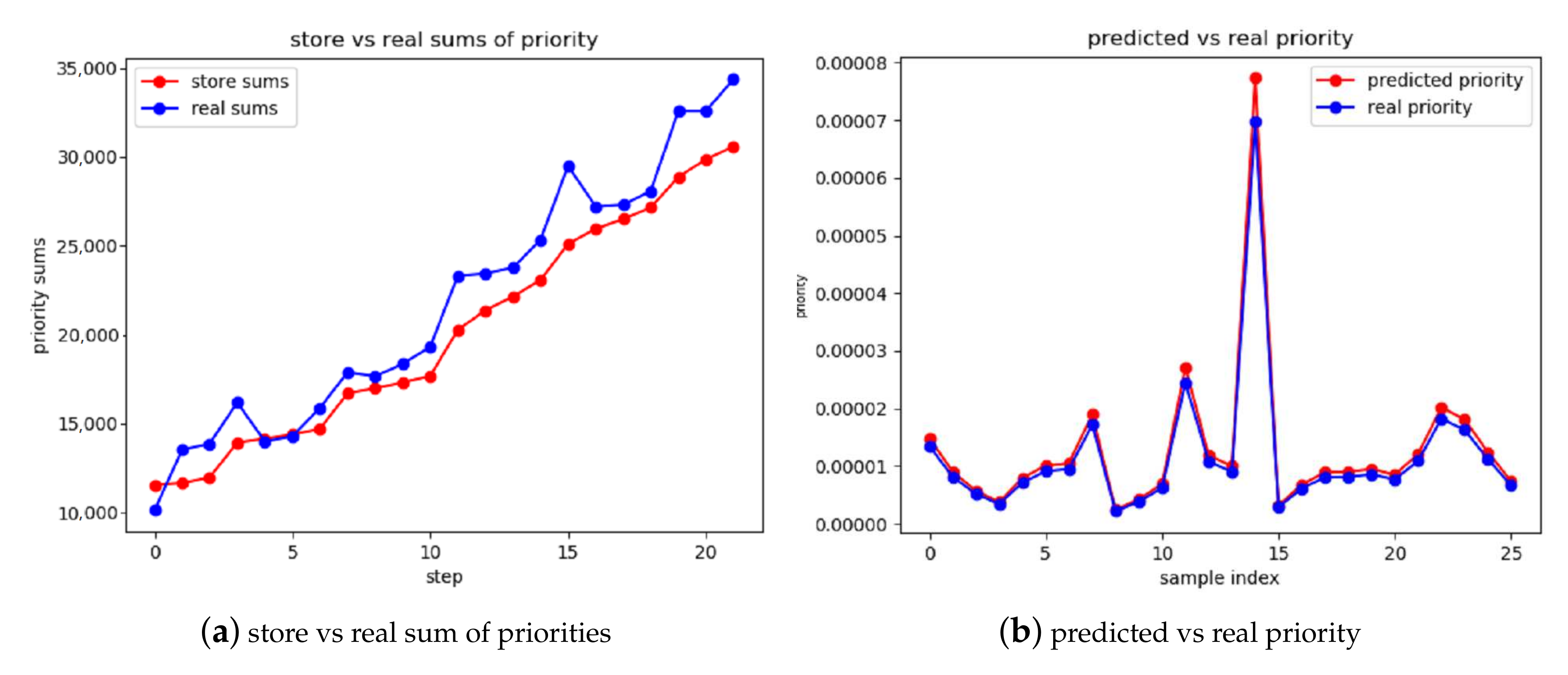
- We design a linear model to predict the sum of real TD-error and estimate the real probability of the current batch of data. Compared to predicting the real probability of each sample in EM, the cost is much less.
- By using IS technology to estimate the DQN or DDPG loss function for the real priority distribution, we improve the data utilization and eliminate the cost of updating the entire EM priority.
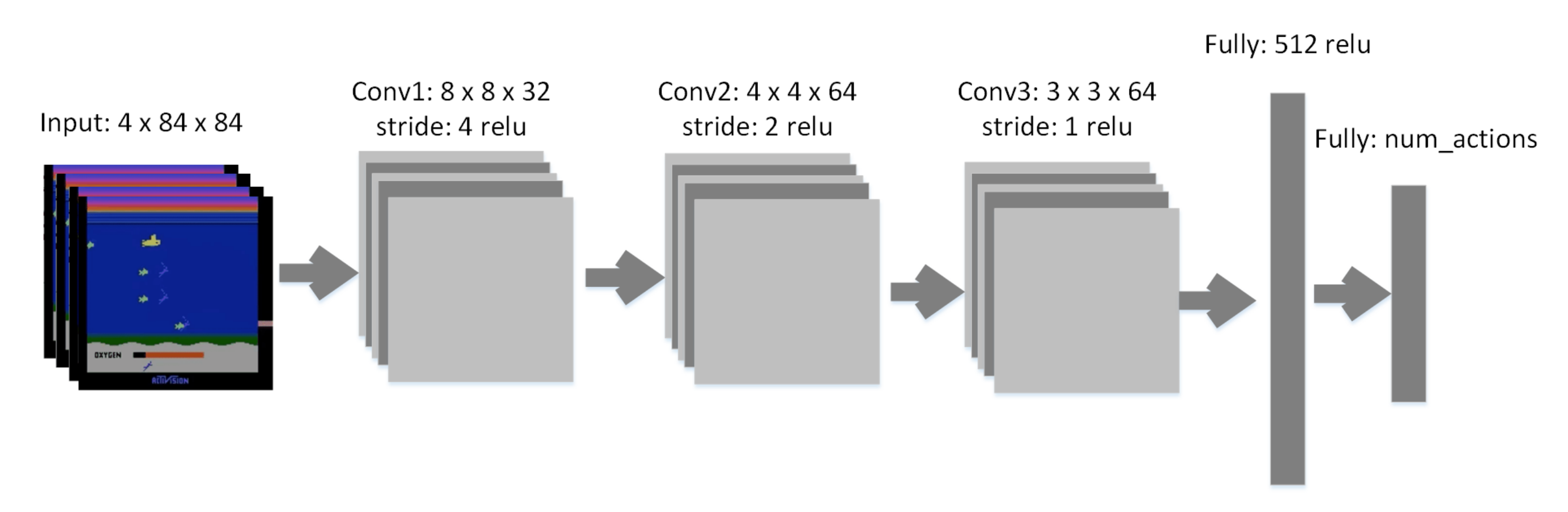
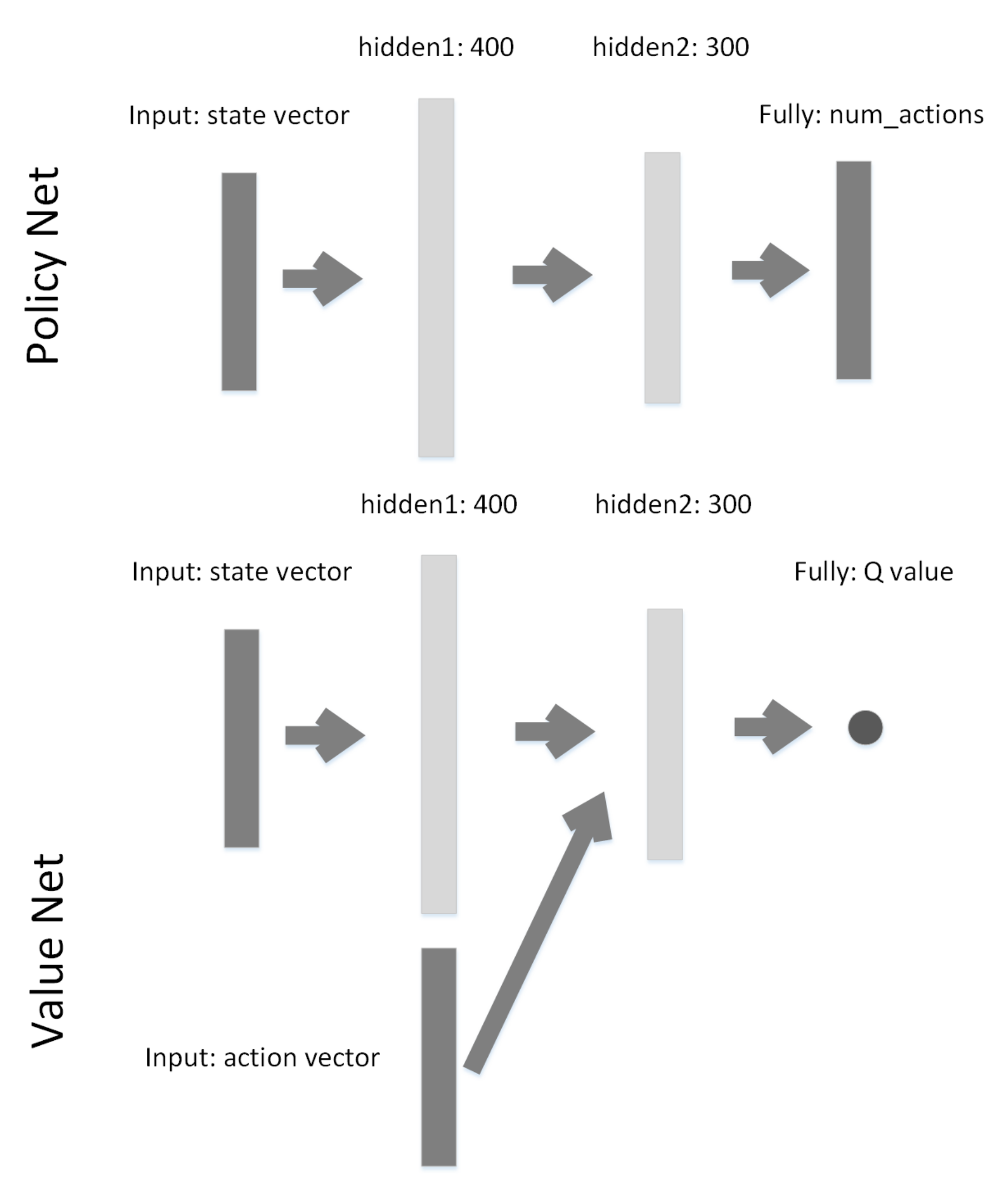
- We conduct experiments on various video games of Atari 2600 with DQN and MuJoCo with DDPG from OpenAI Gym [21] to evaluate our algorithm. Empirical results show that Imp-PER can significantly improve data utilization on discrete state and continuous state tasks without introducing additional computational costs. The experiments also illustrate that Imp-PER is compatible with value-based and policy-based DRL.
2. Related Work
2.1. Priority Experience Replay
2.2. Importance Sampling Techniques
3. Proposed Approach
3.1. Preliminary
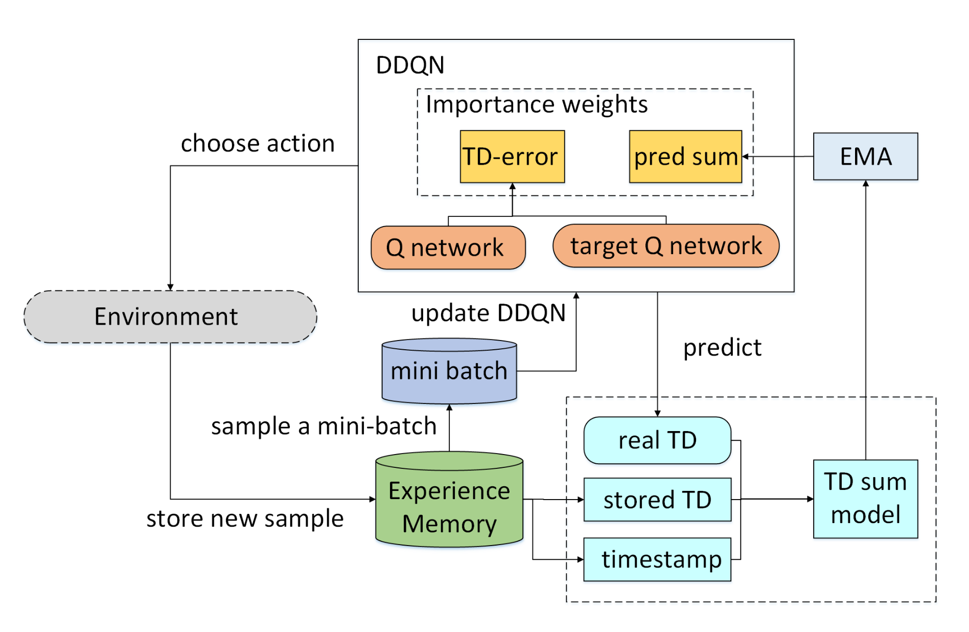
3.2. Overview
3.3. Real Probability Prediction
3.4. Execution Optimization
3.5. Importance Weighted PER
3.6. Algorithm Description
| Algorithm 1 Double DQN with Imp-PER. |
| Input: Linear model update period K, sum predict period D, budget T, mini-batch size k, learning rate , discount factor , importance strength , exponential smoothing , smoothing index , target network update L |
| Output: the parameter of DDQN |
|
4. Experiments
4.1. Experimental Setting
- Vanilla-ER: the original experience replay, where each data is sampled uniform from experience memory.
- Org-PER: the original proportional prioritized experience replay. [9], where each data is sampled according to stored probability.
- ATDC-PER: the latest priority correction algorithm, which uses machine learning to predict the priorities of all data in EM [18].
4.2. Performance Comparison
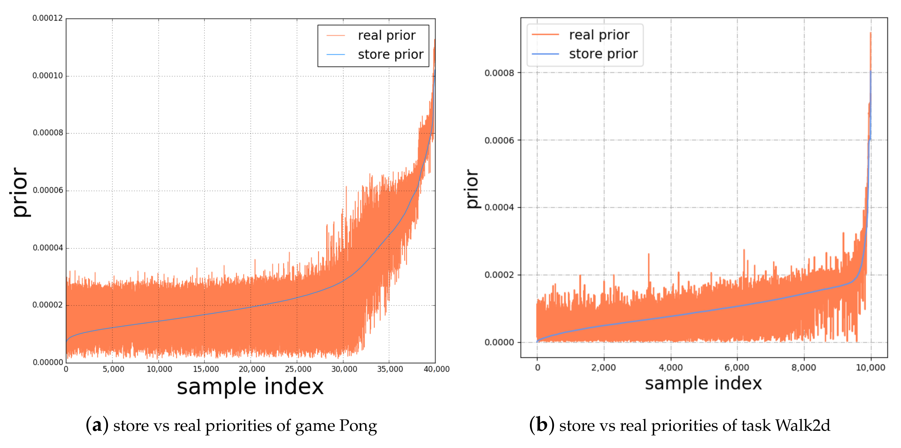
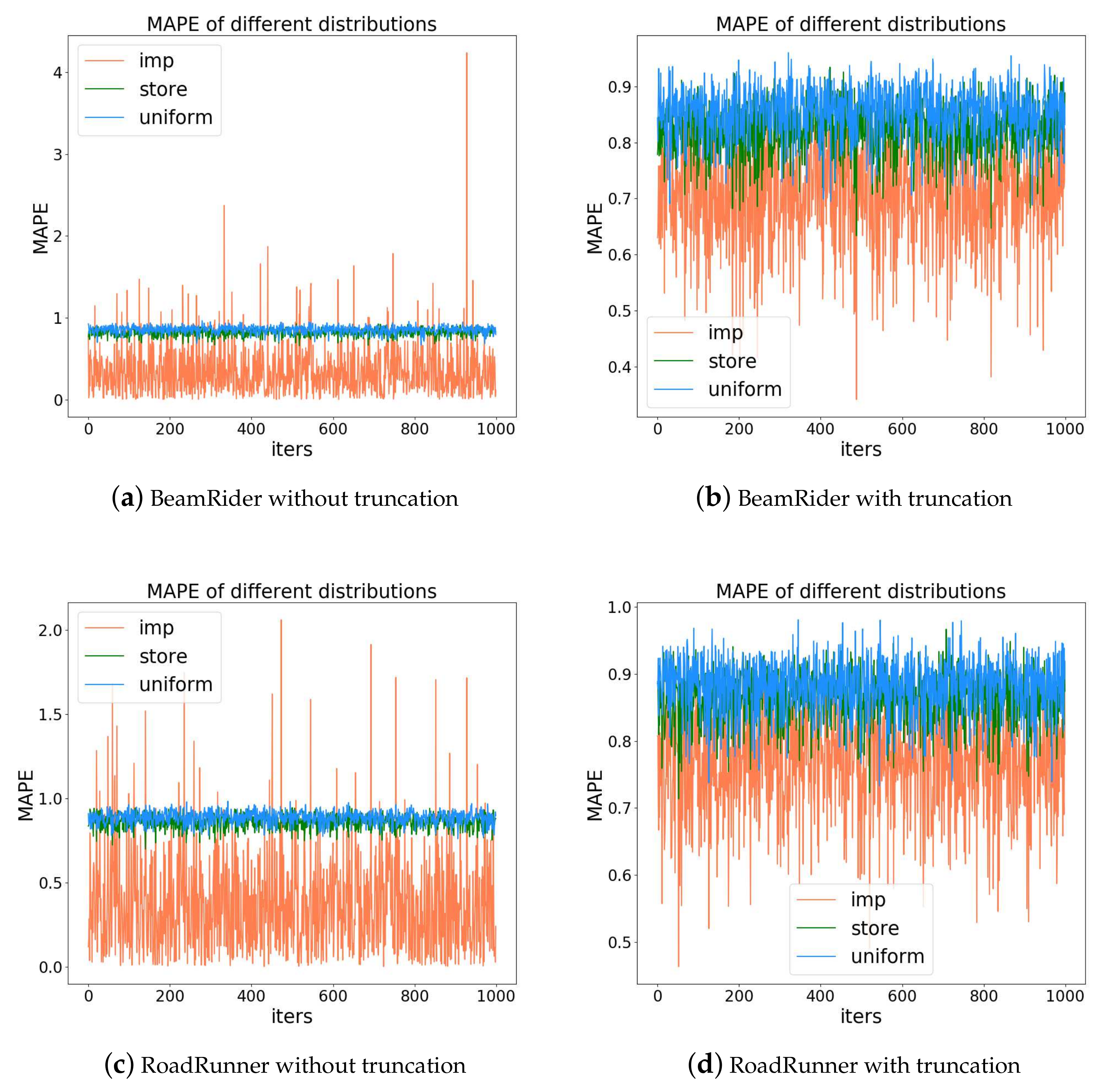
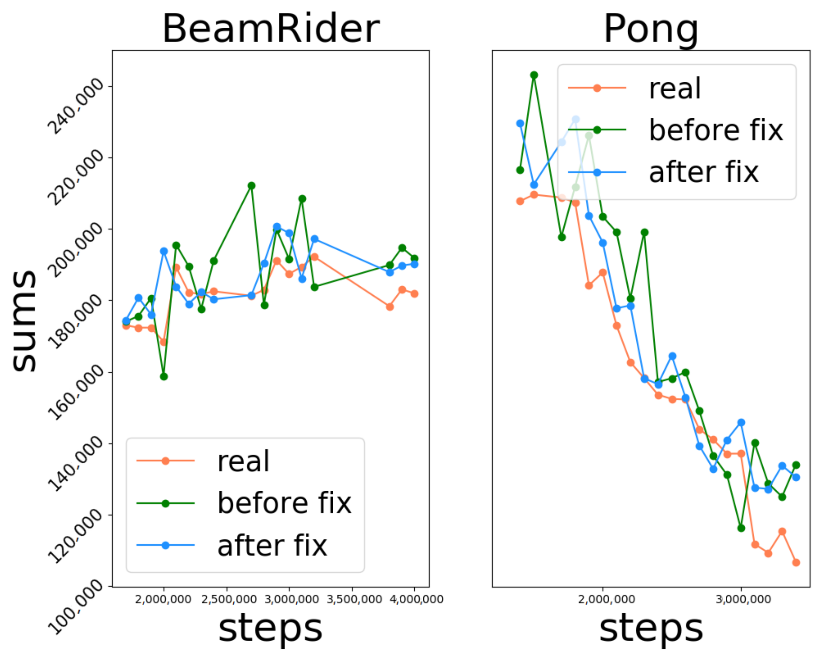
4.2.1. Accuracy of Priority Prediction
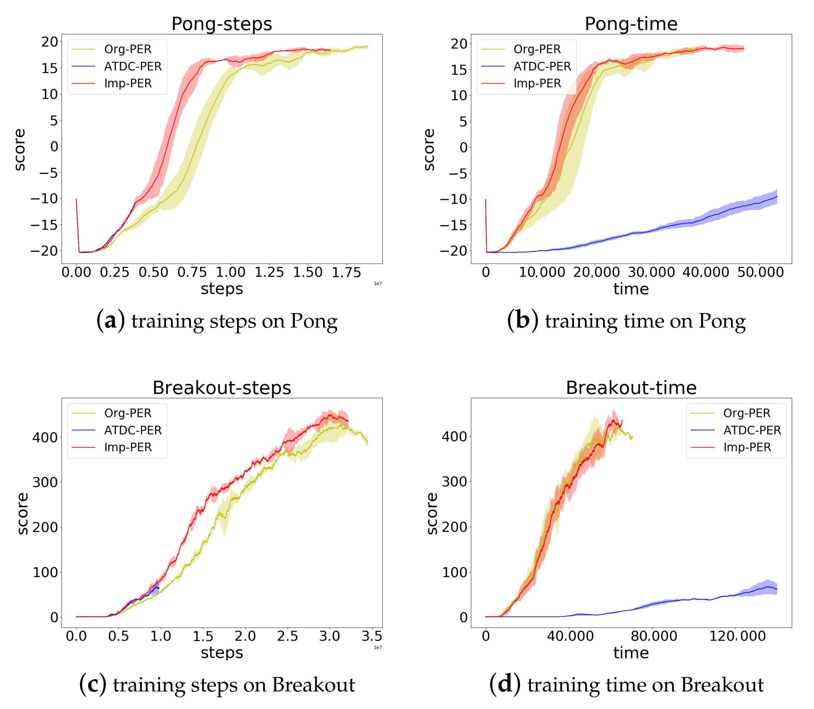
4.2.2. Time Cost Analysis
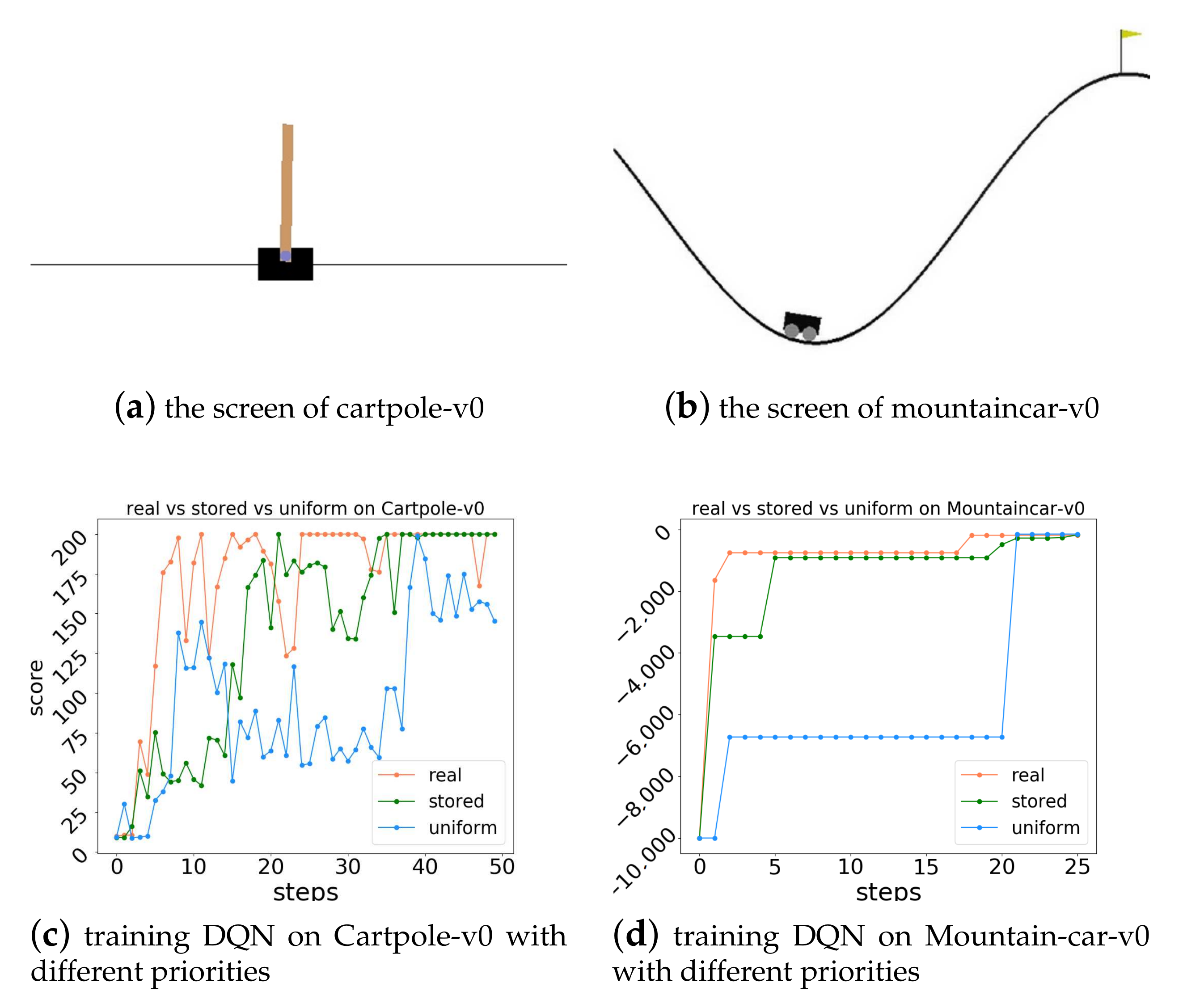
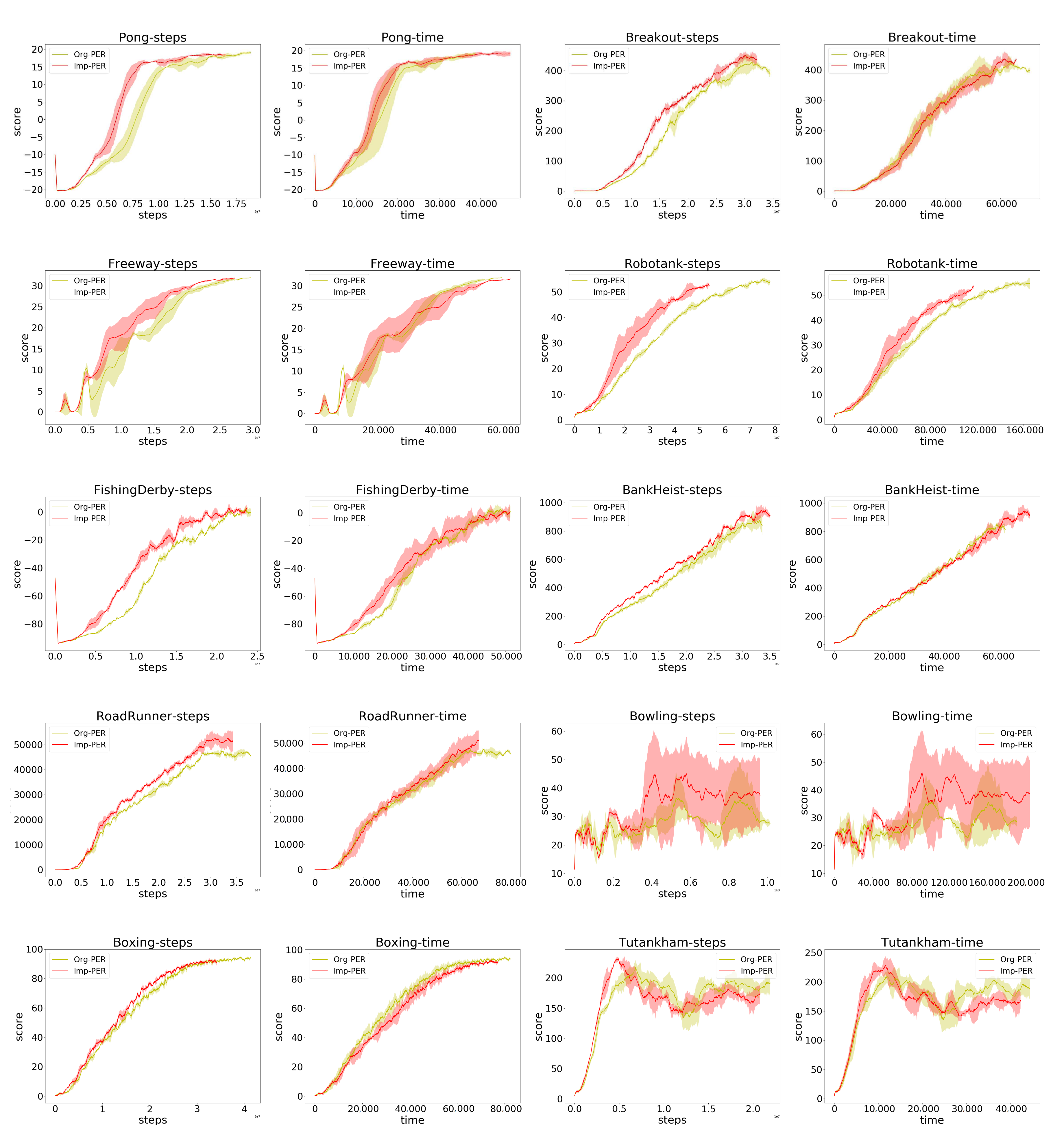
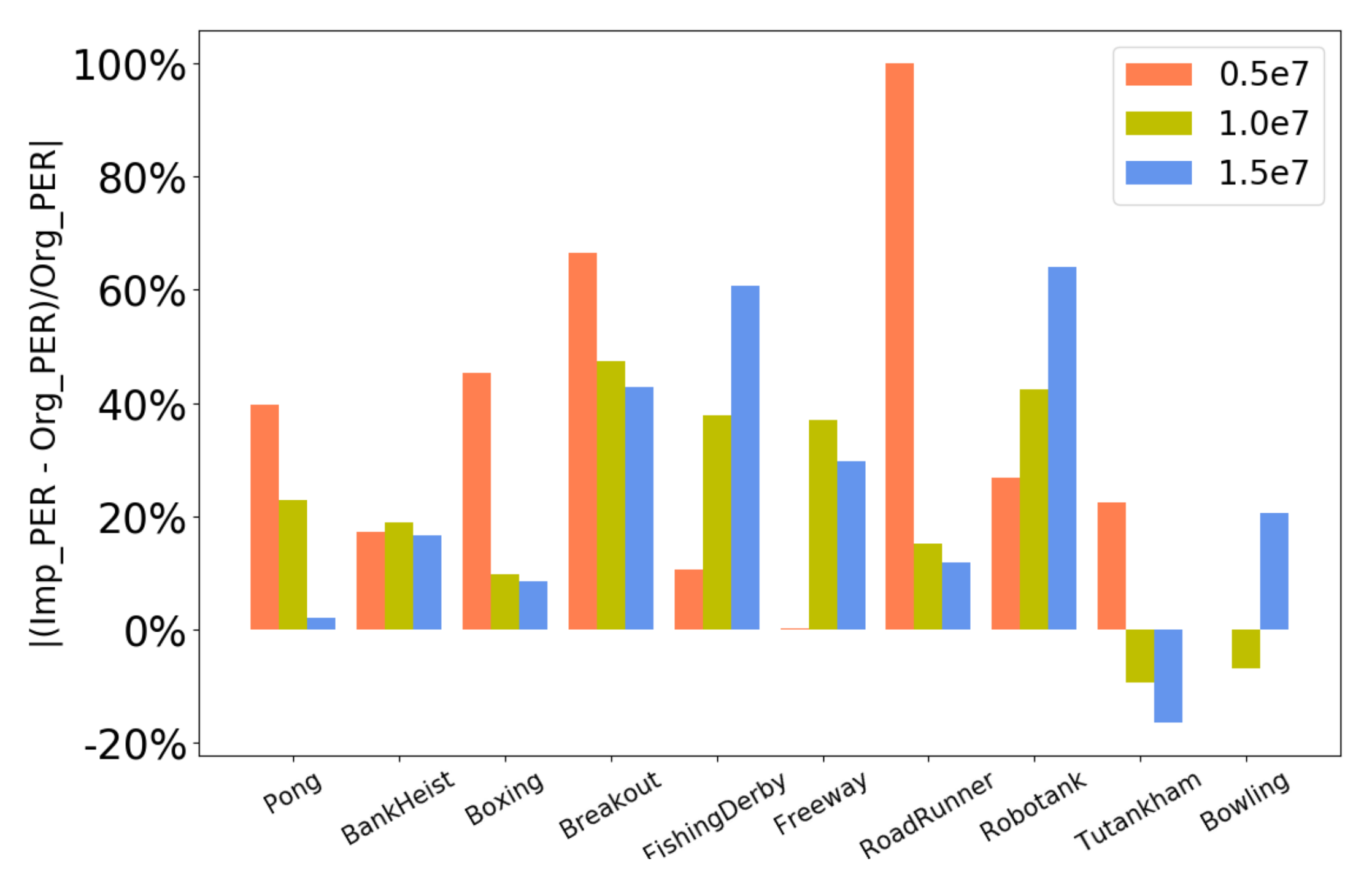
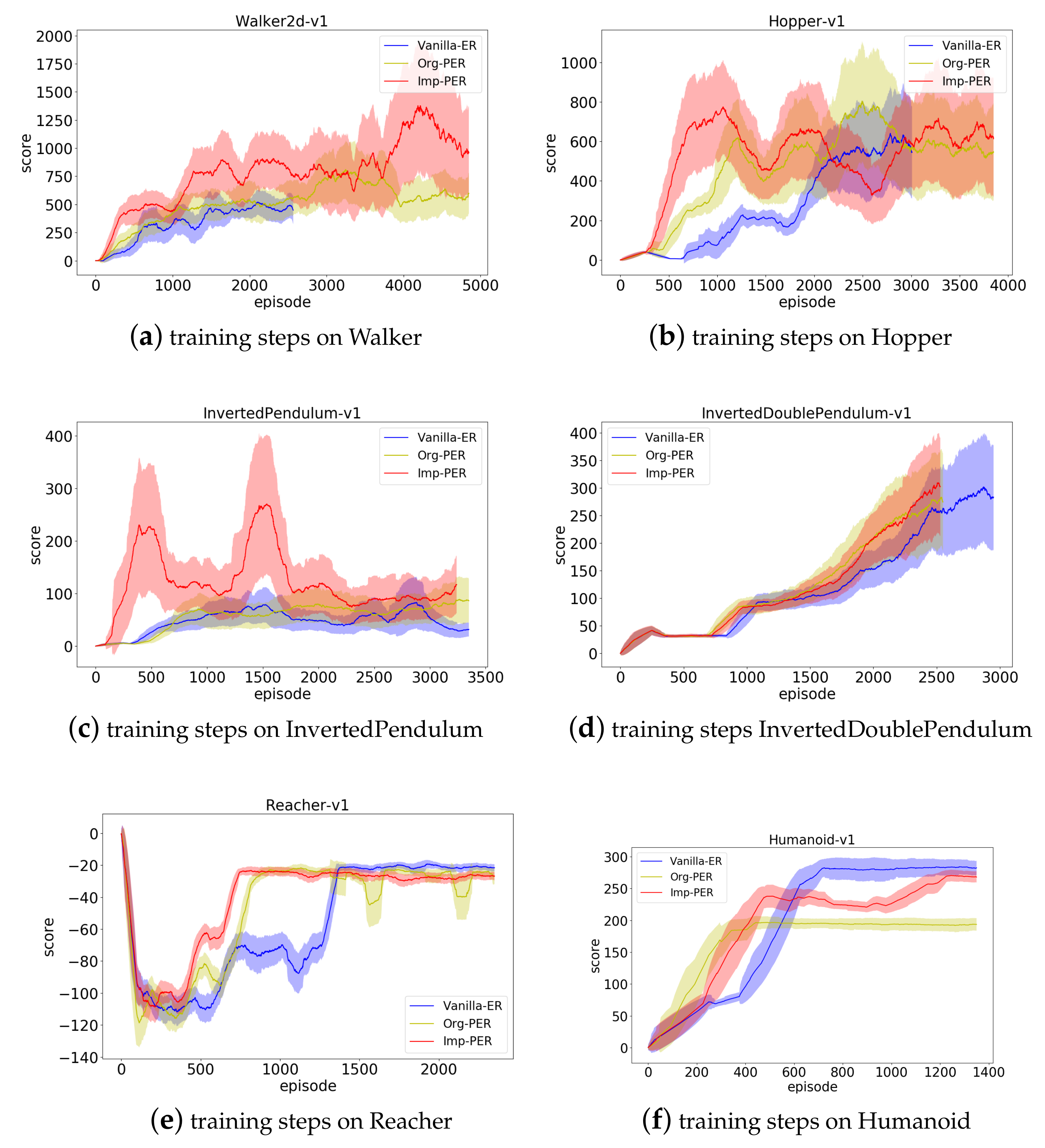
4.2.3. Data Utilization Comparison
4.2.4. Final Policy Quality
5. Conclusions and Future Work
Author Contributions
Funding
Acknowledgments
Conflicts of Interest
References
- Mnih, V.; Kavukcuoglu, K.; Silver, D.; Rusu, A.A.; Veness, J.; Bellemare, M.G.; Graves, A.; Riedmiller, M.; Fidjeland, A.K.; Ostrovski, G.; et al. Human-level control through deep reinforcement learning. Nature 2015, 518, 529–533. [Google Scholar] [CrossRef] [PubMed]
- Wu, H.; Song, S.; You, K.; Wu, C. Depth Control of Model-Free AUVs via Reinforcement Learning. IEEE Trans. Syst. ManCybern. Syst. 2018, 49, 2499–2510. [Google Scholar] [CrossRef]
- Moreira, I.; Rivas, J.; Cruz, F.; Dazeley, R.; Ayala, A.; Fernandes, B. Deep Reinforcement Learning with Interactive Feedback in a Human–Robot Environment. Appl. Sci. 2020, 10, 5574. [Google Scholar] [CrossRef]
- Gregurić, M.; Vujić, M.; Alexopoulos, C.; Miletić, M. Application of Deep Reinforcement Learning in Traffic Signal Control: An Overview and Impact of Open Traffic Data. Appl. Sci. 2020, 10, 4011. [Google Scholar] [CrossRef]
- Silver, D.; Schrittwieser, J.; Simonyan, K.; Antonoglou, I.; Huang, A.; Guez, A.; Hubert, T.; Baker, L.; Lai, M.; Bolton, A.; et al. Mastering the game of Go without human knowledge. Nature 2017, 550, 354–359. [Google Scholar] [CrossRef]
- Chung, H.; Lee, S.J.; Jeon, H.B.; Park, J.G. Semi-Supervised Speech Recognition Acoustic Model Training Using Policy Gradient. Appl. Sci. 2020, 10, 3542. [Google Scholar] [CrossRef]
- Lin, L.-J. Reinforcement Learning for Robots Using Neural Networks; Technical Report; Carnegie Mellon University, School of Computer Science: Pittsburgh, PA, USA, 1993; Available online: https://apps.dtic.mil/dtic/tr/fulltext/u2/a261434.pdf (accessed on 3 July 1993).
- Sutton, R.S.; Barto, A.G. Reinforcement Learning: An Introduction; MIT Press: Cambridge, MA, USA, 2018. [Google Scholar]
- Schaul, T.; Quan, J.; Antonoglou, I.; Silver, D. Prioritized experience replay. In Proceedings of the International Conference on Learning Representations 2016, San Juan, Puerto Rico, 2–4 May 2016. [Google Scholar]
- Van Seijen, H.; Sutton, R.S. Planning by prioritized sweeping with small backups. In Proceedings of the International Conference on Machine Learning 2013, Atlanta, GA, USA, 17–19 June 2013; pp. 361–369. [Google Scholar]
- Horgan, D.; Quan, J.; Budden, D.; Barth-Maron, G.; Hessel, M.; Van Hasselt, H.; Silver, D. Distributed prioritized experience replay. In Proceedings of the International Conference on Learning Representations (ICLR), Vancouver, BC, Canada, 30 April–3 May 2018. [Google Scholar]
- Hou, Y.; Zhang, Y. Improving DDPG via Prioritized Experience Replay; Technical Report; no. May. 2019. Available online: https://course.ie.cuhk.edu.hk/ierg6130/2019/report/team10.pdf (accessed on 5 October 2019).
- Ying-Nan, Z.; Peng, L.; Wei, Z.; Xiang-Long, T. Twice sampling method in deep q-network. Acta Autom. Sin. 2019, 45, 1870–1882. [Google Scholar]
- Zha, D.; Lai, K.H.; Zhou, K.; Hu, X. Experience replay optimization. In Proceedings of the International Joint Conference on Artificial Intelligence 2019, Macao, China, 10–16 August 2019; pp. 4243–4249. [Google Scholar]
- Novati, G.; Koumoutsakos, P. Remember and forget for experience replay. In Proceedings of the International Conference on Machine Learning 2019, Long Beach, CA, USA, 10–15 June 2019; pp. 4851–4860. [Google Scholar]
- Hessel, M.; Modayil, J.; Van Hasselt, H.; Schaul, T.; Ostrovski, G.; Dabney, W.; Horgan, D.; Piot, B.; Azar, M.; Silver, D. Rainbow: Combining improvements in deep reinforcement learning. In Proceedings of the Thirty-Second AAAI Conference on Artificial Intelligence 2018, New Orleans, LA, USA, 2–7 February 2018. [Google Scholar]
- Longji, L. Self-Improving Reactive Agents Based on Reinforcement Learning, Planning and Teaching. Mach. Learn. 1992, 8, 293–321. [Google Scholar]
- Chenjia, B.; Peng, L.; Wei, Z.; Xianglong, T. Active sampling for deep q-learning based on td-error adaptive correction. J. Comput. Res. Dev. 2019, 56, 262–280. [Google Scholar]
- Hesterberg, T.C. Advances in Importance Sampling. Ph.D. Thesis, Stanford University, Stanford, CA, USA, 1988. [Google Scholar]
- Owen, A.B. Monte Carlo Theory, Methods and Examples. 2013. Available online: https://statweb.stanford.edu/~owen/mc/ (accessed on 15 October 2019).
- Brockman, G.; Cheung, V.; Pettersson, L.; Schneider, J.; Schulman, J.; Tang, J.; Zaremba, W. Openai gym. arXiv 2016, arXiv:1606.01540. Available online: https://arxiv.org/abs/1606.01540 (accessed on 1 October 2019).
- Van Hasselt, H.; Guez, A.; Silver, D. Deep reinforcement learning with double q-learning. In Proceedings of the Thirtieth AAAI Conference on Artificial Intelligence, Phoenix, AZ, USA, 12–17 February 2016. [Google Scholar]
- Wang, Z.; Schaul, T.; Hessel, M.; Hasselt, H.; Lanctot, M.; Freitas, N. Dueling network architectures for deep reinforcement learning. arXiv 2015, arXiv:1511.06581. Available online: https://arxiv.org/abs/1511.06581 (accessed on 1 October 2019).
- Cao, X.; Wan, H.; Lin, Y.; Han, S. High-value prioritized experience replay for off-policy reinforcement learning. In Proceedings of the 2019 IEEE 31st International Conference on Tools with Artificial Intelligence (ICTAI), Portland, OR, USA, 4–6 November 2019; pp. 1510–1514. [Google Scholar]
- Hu, C.; Kuklani, M.; Panek, P. Accelerating Reinforcement Learning with Prioritized Experience Replay for Maze Game. SMU Data Sci. Rev. 2020, 3, 8. [Google Scholar]
- Wang, X.; Xiang, H.; Cheng, Y.; Yu, Q. Prioritised experience replay based on sample optimisation. J. Eng. 2020, 13, 298–302. [Google Scholar] [CrossRef]
- Fei, Z.; Wen, W.; Quan, L.; Yuchen, F. A deep q-network method based on upper confidence bound experience sampling. J. Comput. Res. Dev. 2018, 55, 100–111. [Google Scholar]
- Isele, D.; Cosgun, A. Selective experience replay for lifelong learning. In Proceedings of the National Conference on Artificial Intelligence 2018, New Orleans, LA, USA, 2–7 February 2018; pp. 3302–3309. [Google Scholar]
- Zhao, D.; Liu, J.; Wu, R.; Cheng, D.; Tang, X. Optimistic sampling strategy for data-efficient reinforcement learning. IEEE Access 2019, 7, 55763–55769. [Google Scholar] [CrossRef]
- Sun, P.; Zhou, W.; Li, H. Attentive experience replay. In Proceedings of the Thirty-Fourth AAAI Conference on Artificial Intelligence 2020, New York, NY, USA, 7–12 February 2020; pp. 5900–5907. [Google Scholar]
- Bu, F.; Chang, D.E. Double Prioritized State Recycled Experience Replay. arXiv 2020, arXiv:2007.03961. [Google Scholar]
- Yu, T.; Lu, L.; Li, J. A weight-bounded importance sampling method for variance reduction. Int. J. Uncertain. Quantif. 2019, 9, 3. [Google Scholar] [CrossRef]
- Ionides, E.L. Truncated importance sampling. J. Comput. Graph. Stat. 2008, 17, 295–311. [Google Scholar] [CrossRef]
- Thomas, P.S.; Brunskill, E. Importance sampling with unequal support. In Proceedings of the National Conference on Artificial Intelligence 2016, Phoenix, AZ, USA, 12–17 February 2016; pp. 2646–2652. [Google Scholar]
- Martino, L.; Elvira, V.; Louzada, F. Effective sample size for importance sampling based on discrepancy measures. Signal Process. 2017, 131, 386–401. [Google Scholar] [CrossRef]
- Chatterjee, S.; Diaconis, P. The sample size required in importance sampling. Ann. Appl. Probab. 2018, 28, 1099–1135. [Google Scholar] [CrossRef]
- Andre, D.; Friedman, N.; Parr, R. Generalized prioritized sweeping. In Proceedings of the Advances in Neural Information Processing Systems 1998, Denver, CO, USA, 30 November–5 December 1998; pp. 1001–1007. [Google Scholar]
- Bellemare, M.G.; Naddaf, Y.; Veness, J.; Bowling, M. The arcade learning environment: An evaluation platform for general agents. J. Artif. Intell. Res. 2013, 47, 253–279. [Google Scholar] [CrossRef]
- Dhariwal, P.; Hesse, C.; Klimov, O.; Nichol, A.; Plappert, M.; Radford, A.; Schulman, J.; Sidor, S.; Wu, Y.; Zhokhov, P. Openai Baselines; GitHub Repository; GitHub: San Francisco, CA, USA, 2017. [Google Scholar]
- Abadi, M.; Barham, P.; Chen, J.; Chen, Z.; Davis, A.; Dean, J.; Devin, M.; Ghemawat, S.; Irving, G.; Isard, M.; et al. Tensorflow: A system for largescale machine learning. In Proceedings of the 12th USENIX Symposium on Operating Systems Design and Implementation (OSDI 16), Savannah, GA, USA, 2–4 November 2016; pp. 265–283. [Google Scholar]
- De Myttenaere, A.; Golden, B.; Le Grand, B.; Rossi, F. Mean absolute percentage error for regression models. Neurocomputing 2016, 192, 38–48. [Google Scholar] [CrossRef]


| Hyparameter | Memory | Batch Size | Target Q | |||||
|---|---|---|---|---|---|---|---|---|
| Value | 0.6 | 0.4→1.0 | 32 | 0.99 | 0.0001 | 40,000 | 0.0→1.0 |
| Hyparameter | Memory | Batch Size | Noise | Noise | ||||
|---|---|---|---|---|---|---|---|---|
| Value | 0.6 | 0.4→1.0 | 32 | 0.99 | 0.0001 | 0.2 | 0.15 |
| Methods | |||
|---|---|---|---|
| ATDC-PER | 76 | 54 | 48 |
| Imp-PER | 6 | 3 | 0.7 |
| Method | Total | Sampling | Update | DDQN |
|---|---|---|---|---|
| Org-PER | 0.014 | 0.005 | 0.0028 | 0.006 |
| ATDC-PER | 0.150 | 0.075 | 0.0028 | 0.006 |
| Imp-PER | 0.015 | 0.005 | 0.0029 | 0.007 |
| Game | Org-PER | Imp-PER | ||||
|---|---|---|---|---|---|---|
| Pong | −12.1 | 13.5 | 18.6 | 7.3 | 16.6 | 19 |
| BankHeist | 151.8 | 279.2 | 400 | 178.2 | 332 | 466.6 |
| Boxing | 11.9 | 34.6 | 55.3 | 17.3 | 38 | 60 |
| Breakout | 10 | 63.27 | 174.9 | 16.65 | 93.24 | 249.95 |
| FishingDerby | −87.15 | −64.29 | −20 | −77.85 | −40 | −7.86 |
| Freeway | 8.3 | 13.57 | 19.28 | 8.33 | 18.6 | 25 |
| RoadRunner | 2000 | 18,400 | 26,800 | 4000 | 21,200 | 30,000 |
| Robotank | 3.64 | 7.3 | 13.1 | 4.62 | 10.4 | 21.5 |
| Tutankham | 187 | 183 | 187 | 229 | 166.1 | 156.4 |
| Bowling | 25 | 22 | 20.3 | 25 | 20.5 | 24.5 |
| Game | Uniform | Human | Raw Score | Normalized Score % | ||||
|---|---|---|---|---|---|---|---|---|
| DDQN | Org-PER | Imp-PER | DDQN | Org-PER | Imp-PER | |||
| BankHeist | 21.7 | 644.5 | 728.3 | 870.6 | 951.6 | 113.4 | 136.3 | 149.3 |
| Bowling | 35.2 | 146.5 | 50.4 | 53.5 | 60.5 | 13.6 | 16.4 | 22.7 |
| Boxing | −1.5 | 9.6 | 81.7 | 90.6 | 90.3 | 749.5 | 829.7 | 827.0 |
| Breakout | 1.7 | 31.8 | 450 | 420.5 | 451.3 | 1489.3 | 1391.3 | 1493.6 |
| FishingDerby | −77.1 | 5.1 | 3.2 | 3.1 | 3.4 | 97.6 | 97.5 | 97.9 |
| Freeway | 0.1 | 25.6 | 28.8 | 32 | 32.2 | 112.5 | 125.0 | 125.8 |
| Pong | −20.7 | 9.3 | 21 | 20.7 | 21 | 139 | 138 | 139 |
| RoadRunner | 11.5 | 7845 | 48,330.5 | 50,113 | 54,370.6 | 616.8 | 639.5 | 693.9 |
| Robotank | 2.2 | 11.9 | 47.8 | 53.7 | 52.1 | 470.1 | 530.9 | 514.4 |
| Tutankham | 12.7 | 138.3 | 125.7 | 207 | 190 | 89.9 | 154.6 | 141.1 |
| Metrics | DDQN | Org-PER | Imp-PER |
|---|---|---|---|
| Median | 113.4 | 138 | 141.1 |
| Mean | 389.2 | 405.9 | 420.5 |
| Tasks | Random | Vanilla-ER | Org-PER | Imp-PER | Relative Improvement |
|---|---|---|---|---|---|
| Walker2d | −4.34 | 500 | 800 | 1360 | 70% |
| Hopper | 11 | 650 | 800 | 950 | 18.8% |
| InvertedPendulum | 7.76 | 120 | 105 | 275 | 161.9% |
| InvertedDoublePendulum | 54.11 | 300 | 275 | 312 | 13.5% |
| Reacher | −90 | −9 | −10 | −10 | 0% |
| Humanoid | 102.01 | 284 | 195 | 271 | 38.97% |
© 2020 by the authors. Licensee MDPI, Basel, Switzerland. This article is an open access article distributed under the terms and conditions of the Creative Commons Attribution (CC BY) license (http://creativecommons.org/licenses/by/4.0/).
Share and Cite
Zhang, H.; Qu, C.; Zhang, J.; Li, J. Self-Adaptive Priority Correction for Prioritized Experience Replay. Appl. Sci. 2020, 10, 6925. https://doi.org/10.3390/app10196925
Zhang H, Qu C, Zhang J, Li J. Self-Adaptive Priority Correction for Prioritized Experience Replay. Applied Sciences. 2020; 10(19):6925. https://doi.org/10.3390/app10196925
Chicago/Turabian StyleZhang, Hongjie, Cheng Qu, Jindou Zhang, and Jing Li. 2020. "Self-Adaptive Priority Correction for Prioritized Experience Replay" Applied Sciences 10, no. 19: 6925. https://doi.org/10.3390/app10196925
APA StyleZhang, H., Qu, C., Zhang, J., & Li, J. (2020). Self-Adaptive Priority Correction for Prioritized Experience Replay. Applied Sciences, 10(19), 6925. https://doi.org/10.3390/app10196925