Acoustic-Based Engine Fault Diagnosis Using WPT, PCA and Bayesian Optimization

Featured Application

In this paper, the proposed method is validated using experimental studies based on sound signals for engine fault diagnosis, though ultimately the developed framework can be widely applicable to many other industrial fault diagnosis scenarios, e.g., in aeronautical, automotive, energy and manufacturing industry. 

Abstract

Engine fault diagnosis aims to assist engineers in undertaking vehicle maintenance in an efficient manner. This paper presents an automatic model and hyperparameter selection scheme for engine combustion fault classification, using acoustic signals captured from cylinder heads of the engine. Wavelet Packet Transform (WPT) is utilized for time–frequency analysis, and statistical features are extracted from both high- and low-level WPT coefficients. Then, the extracted features are used to compare three models: (i) standard classification model; (ii) Bayesian optimization for automatic model and hyperparameters selection; and (iii) Principle Component Analysis (PCA) for feature space dimensionality reduction combined with Bayesian optimization. The latter two models both demonstrated improved accuracy and the other performance metrics compared to the standard model. Moreover, with similar accuracy level, PCA with Bayesian optimized model achieved around 20% less total evaluation time and 8–19% less testing time, compared to the second model, for all fault conditions, which thus shows a promising solution for further development in real-time engine fault diagnosis.

1. Introduction

Internal Combustion Engines (ICEs) are the major power source for a variety of application including automobiles, aircraft, marine units, lighting plants, machine tools, power tool, etc. According to JATO report, ICEs account for 91% of the passenger car global sales in 2019 [1]. In order for the vehicle manufactures to comply with increasingly stringent regulations, there is a need to maintain the overall efficiency, performance and emission level in an ICE. Thus, it is always crucial to run an engine in optimal conditions. This can be achieved by the use of the condition-based maintenance scheme for emergent fault diagnosis or detecting any deviations from optimal conditions.

An ICE has various rotating and moving parts, which over time can degrade due to extreme operating conditions. For instance, a spark ignition engine, which is a type of ICE, is subject to maintenance issues such as aged spark plug, damaged oxygen sensor or prolonged knocking, which can deteriorate the performance of the engine or even worse can cause total engine failure in the long run [2]. Fault detection systems can help identify these faults at an early stage and reduce further damage to the engine, thereby increasing safety and reliability of the vehicle.

Fault diagnosis methods have been categorized into two main types: signal-based and model-based methods [3]. In this study, we used a signal-based method which includes extracting useful features and comparing them against those of the nominal operational conditions using acoustic information from ICEs. Signal-based methods are less complex, easier to implement and more flexible to operation changes compared to model-based fault diagnosis methods.

Information from ICEs can be gathered in various formats such as acoustic signals, vibration [4], oil quality [5] and thermal images [6], which are widely studied for engine fault diagnosis. Other analysis techniques include in-cylinder pressure mapping [7] and instantaneous angular speed measurement [8], which can be tedious and expensive. Recently, acoustic signals have gained increased attention for engine fault diagnosis because of the capacity of taking measurements from a distance, avoiding safety risks and removing the need of temperature sensitive sensors in the case of vibration [9]. Acoustic analysis has not been used widely in the past due to the fact that these signals are susceptible to high noise content and are easily influenced by local environment. However, this could be mitigated through the use of sophisticated signal processing, denoising and feature mining techniques to extract useful information from a contaminated signal.

The signal-based fault diagnosis system consists of mainly four phases: data collection, signal decomposition, feature extraction and fault condition classification [10]. The traditional signal processing approach uses time-domain and frequency-domain analysis to distinguish different fault conditions. For example, the authors of [11] used frequency-domain analysis, including Fast Fourier Transform (FFT), envelope analysis and order tracking, for the recognition of different operating conditions and fault types. The major disadvantage of FFT-based approaches is that it is not adequate to analyze the time-dependent elements in the frequency domain only. This issue can be solved through the use of time–frequency analysis methods, such as Short-time Fourier Transform (STFT) [12] and wavelet transform. Wavelet transform is particularly effective compared to STFT because of its capability of analyzing signals in multi-resolution time–frequency windows. Therefore, it is been used widely for fault diagnosis of engines [13,14,15,16,17]. Although many variations of wavelet transform exist, in this paper, Wavelet Packet Transform (WPT) is used because WPT can transform the signal into both high- and low-level wavelet coefficients. This is significant, since various fault types embedded in different frequency ranges are analyzed here [18,19]. After signal decomposition, relevant time–frequency information can be extracted, and it can be used as the input for fault classification.

Most fault diagnosis models in the literature follow a single classification algorithm or attempt to compare among few classification algorithms to find the best model [20,21,22,23]. However, it has to be noted that each emerging fault has different characteristics and the appropriate algorithm has to be chosen according to their corresponding classification performance. There has been considerable work on optimization of model hyperparameters [24,25]. However, there are limited approaches for the combined model selection with hyperparameter optimization in literature. One useful methodology is the utilization of meta learning procedures which employ information from previous data to find the optimal algorithm or hyperparameter configuration [26]. This is not practical in many cases due to its computational complexity in evaluating a huge amount of previous data. Bayesian optimization is an adequate method to overcome this issue [27], which has been shown to outperform other optimization techniques on several of challenging benchmark problems [28,29]. The objective of Bayesian optimization is to find a point that minimizes an objective function using cross-validation classification error [30,31]. The function evaluation itself could involve an onerous procedure, and this is addressed in [30] by using a conventional dimensionality reduction technique—Principle Component Analysis (PCA). By reducing the feature space to smaller number of Principle Components (PCs), the computational complexity is reduced, lowering the evaluation time [32,33]. PCA has been proven to reduce training time and improve the classification performance in very large datasets as shown in [34]. Nonetheless, the utilization of PCA to reduce the feature set for Bayesian optimization and its effect on the optimization performance have not been addressed critically in the known literature.

The aim of this paper is to present a new fault diagnosis method for a gasoline ICE with various fault conditions by analyzing its acoustic signals. This starts with Model 1, which contains the selection of standard classifiers. It evolves to Model 2, which uses Bayesian optimization for both model selection and model hyperparameter optimization, so that an optimal model with its selected features and parameters is provided. Finally, Model 3 is proposed, which applies PCA alongside Bayesian optimization to reduce the complexity of the feature space for the optimization problem. All three models use WPT for signal analysis and the statistical features computed from the high- and low-level WPT coefficients. Hence, the main contributions of this paper are as follows:

• Exploring the viability of the use of acoustic signals for engine fault classification under different fault scenarios and different operating conditions
• Evaluating the performance and the use of Bayesian optimization on standard classification models for fault diagnosis of an ICE
• Evaluating the effect of PCA on the optimized fault classification model in terms of classification accuracy, other performance metrics and the evaluation time

The remainder of this paper is structured as follows. Section 2 presents the experimental set up and the engine fault characteristics. Section 3 describes the general workflow and the detailed methodology employed. Section 4 describes the results and the comparison of the three models using various performance metrics. Section 5 concludes the paper.

2. Experimental Work

2.1. Gasoline Engine and Data Acquisition System

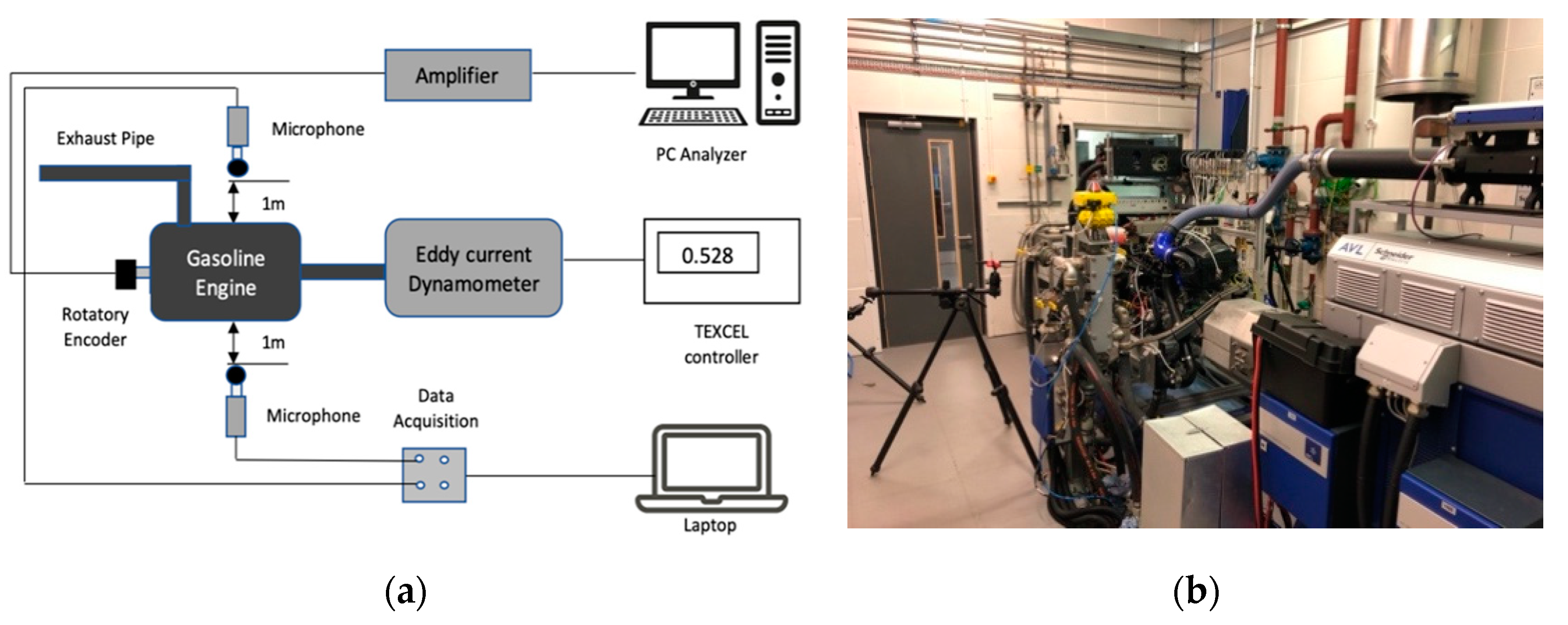
The experimental works were carried out using a Ford-Eco Boost 1.6 L which is mainly used in Ford Focus, Ford Fiesta and Transit Courier. The specifications of the ICE are provided in Table 1. The engine is fully instrumented to measure all operating conditions including speed, load, cylinder pressure, injection pressure, etc. It also has the ability to change parameters such as injection timing, pressure, etc., as well as to cut off cylinders during run, as shown in Figure 1.

Table 1. Engine specifications.

	Ford-Eco Boost 1.6L
Engine type	4-stroke GDI with turbocharger
No. of Cylinders	4 Cylinder
Compression Ratio	10.1:1
Engine capacity	1596 cm3
Power	132 KW @ 6000 rpm
Torque	178 Nm @ 2500 rpm
Firing order	1-3-4-2

Figure 1. (a) Schematic of the set-up; and (b) the instrumented engine.

Acoustic signals were collected using microphones. It was carried out by two Vernier MCA-BTA sensors mounted 1 m from the cylinder head on left and right side, as shown in the Figure 1a. The microphones were fed to a five-channel data logger, Labquest 2, which was connected to the laptop. Acoustic signals were also captured by mobile phones, iPhone 6s, with a sampling frequency of 44.1 kHz. Each dataset comprised 10 s of vibration signals with 441,000 data points. The audio sample has a bit rate of 128 kb/s with mono-channel. Vision 4.1.4 version was used for data acquisition for varying engine parameters.

Three types of failures were experimented and injected into the engine, where each experiment was done at different speeds and different loading conditions. These include:

• Engine misfire
• Ignition timing variation
• Air Fuel Ratio (AFR) variation

Engine misfire is a common defect in engines. This fault was replicated by cutting off one of the cylinders, which effectively gave no combustion into a cylinder. The next fault is ignition timing variation, which was replicated by varying the ignition timing from 15° retarded to 15° advanced from the manufacture recommended setting for different operating conditions. Lastly, AFR variation is a critical fault, as it makes real time adjustments to fuel and timing for maximum efficiency and power, and damage to AFR sensor or air flow meter can cause drop in engine efficiency and power output. This was replicated by varying the air mass flow rate. The resultant AFR and lambda, which is the ratio of actual AFR to the stoichiometric ratio, were obtained. The AFR was varied from 10.10 to 17.20 with stoichiometric at 14.45. The test engine was operated under different operating conditions to diversify the data. The various operating points are given in Table 2.

Table 2. Fault seeding and operating conditions.

Type of Engine Data		Engine Speed [rpm]	Load Torque [Nm]	Damage (Main Mode &Symptoms)
Engine Misfire	Healthy	925 (Idle)	0	-
		1750	0.15
	Faulty	925 (Idle)	0	Cylinder 3 Cut off
		1750	0.15
Ignition Timing Variation	Healthy	2250	0.5	Ignition timing at 20.4°
	Advance	2250	0.5	Ignition timing at 5.4°
	Retard			Ignition timing at 35.4°
AFR Variation	Healthy	3000	0.5	AFR at 14.45
	Lean	3000	0.5	AFR at 10.10
	Rich			AFR at 17.20

2.2. Basic Signal Analysis

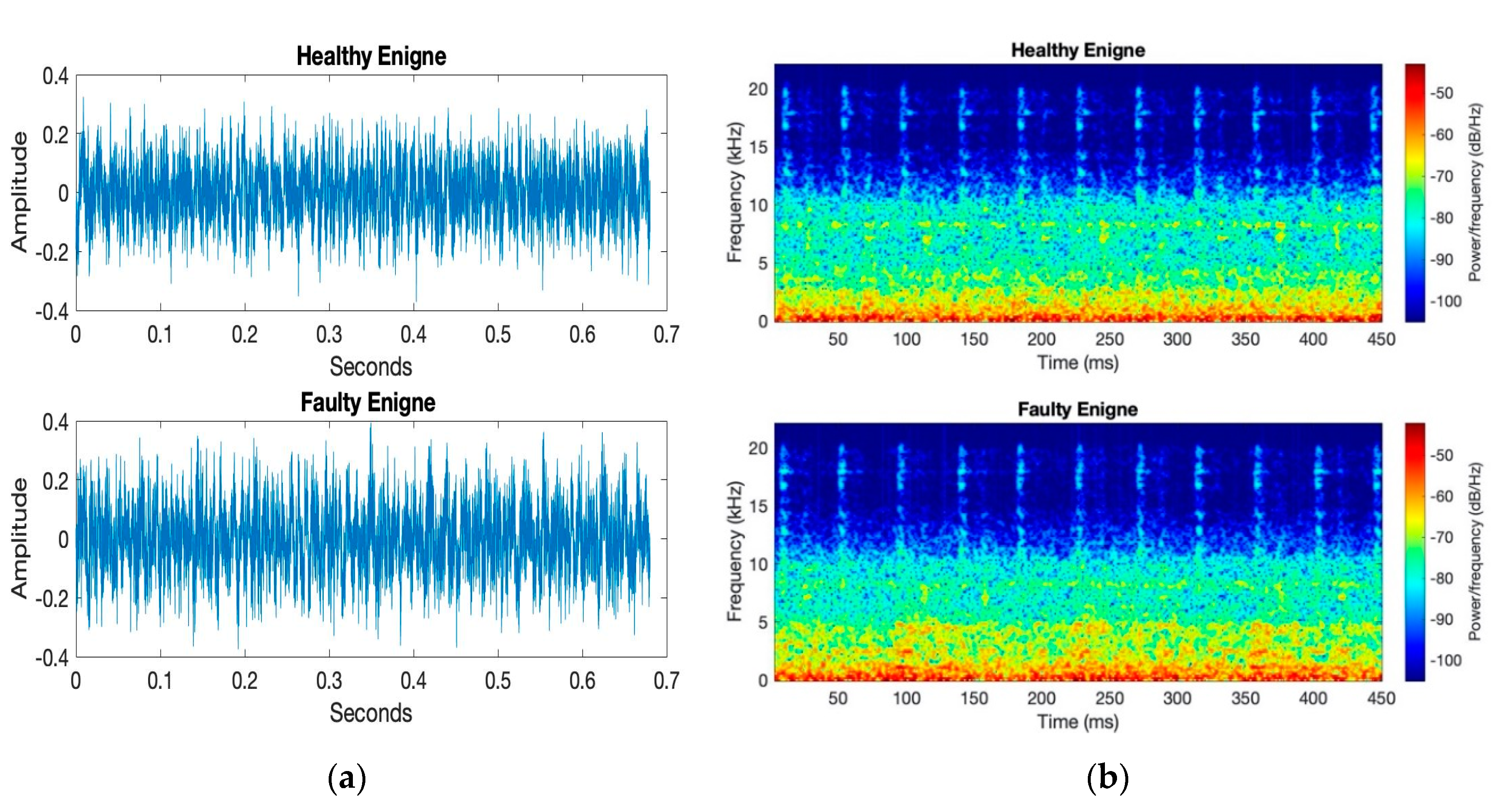
Time-domain data were analyzed for all the cases to understand the characteristics of the signals. The time-domain signals of the engine misfire case are shown in Figure 2a, which shows no conceivable difference between healthy and fault signals. The spectrogram is presented in Figure 2b, which reveals that differentiation between the healthy and the faulty engine is more discernable. The variation can be perceived in every third firing order since the third cylinder was cut off. However, in the case of more complex faults such as ignition timing variation, as shown in Figure 3, the difference becomes more inconceivable. Based on the spectrogram analysis, it can be seen that complex faults require more advanced investigations rather than basic time–frequency domain analysis. Thus, further analyses are presented in the following section for improved fault detection and classification.

Figure 2. Engine misfire—healthy and faulty: (a) signals; and (b) spectrogram.

Figure 3. Ignition timing variation—healthy and faulty: (a) signals; and (b) spectrogram.

3. Methodology

The main objective was to develop and experimentally validate an adaptive fault detection and classification system for vehicles that is robust to different speeds and operating conditions. The acoustic signals were collected from the engine and preprocessed, where the signal was decomposed using WPT and the feature vectors were using statistical measures of the wavelet coefficients. Three models were analyzed and compared—from standard classifiers (Model 1) to Bayesian optimized classification model (Model 2) and finally to PCA combined with Bayesian optimized model (Model 3). A generalized workflow is demonstrated in Figure 4.

Figure 4. Workflow of the methodology and the comparisons for engine fault diagnosis.

Model 1 uses standard classification models. Model 2 uses Bayesian optimization for auto classification model selection and hyperparameter optimization. Finally, Model 3 uses PCA alongside Bayesian optimization to reduce the dimensionality of the large feature matrix and ensure good accuracy with reduced computational complexity and evaluation time.

3.1. Signal Processing

ICE noise primarily consists of combustion, mechanical and aerodynamic noise. Combustion noise is important in the engine noise at low and medium rotating speeds, while mechanical noise dominates the engine noise at higher speeds [35,36]. Combustion noise is intrinsically transient in nature, which is heavily influenced by the injection parameters, spark timing and AFR. Therefore, it is essential to evaluate these signals with the help of time–frequency analysis. Several time–frequency analysis methods are commonly available, such as Gabor transform, STFT, Wigner–Ville transform and wavelet transform. Among these, WPT is of particular interest due to its ability to detect rapidly changing amplitude and phase characteristics [37]. It is a form of wavelet transform, which can decompose a temporal signal into several independent time–frequency vectors termed packets.

In brief, the wavelets are created from scaling and shifting of the mother wavelet. The decomposition results in discrete approximation coefficients low frequency components and detail coefficients high frequency components, using high and low pass filters. There are a number of mother number wavelets that can be used to analyze a signal, the selection of which depends on the signal type and the nature of the application. Among them, Daubechies wavelets are a group of orthogonal wavelets commonly used for discrete wavelet transform which are useful for analyzing transient signals [13]. In this case, Db4 (Daubechies 4) WPT with four layers and a filtering frequency of 12 kHz are used for further analysis. This procedure enables selecting only the optimal components frequency ranges for analysis of different fault conditions.

3.2. Feature Extraction

Features can be extracted from the decomposed signals that can be used further as input by the classification model to distinguish various signals—healthy and faulty, for instance. In this study, eight statistical features were used for feature extraction based on 16 sets of WPT Level 4 coefficients. Thus, after decomposition, for each coefficient, the statistical features in Table 3 were calculated. The total number of features totaled 8 × 16 = 128. The initial dataset for ignition timing variation and AFR variation contains 300 instances and that for engine misfire contains 200 instances for different conditions. Thus, we have the feature matrix of 300 × 128 or 200 × 128 depending on the type of fault.

Table 3. Description and formulae for important statistical features.

Feature	Equations of the Detail & Approximation Coefficients
Mean	$\mu =\frac{1}{N} {\displaystyle {\displaystyle \sum }_{i=1}^N}{x}_i$
Standard Deviation	$\sigma =\sqrt{\frac{1}{N}{\displaystyle {\displaystyle \sum }_{i=1}^N}{\left(x_i-\mu \right)}^2}$
Maximum	Maximum value or the peak of the given signal or its coefficients.
Sum of Peaks	Sum of first 5 peaks of the given signal or its coefficients.
Skewness	$x_{skewness}=\frac{1}{N}\frac{{{\displaystyle \sum }}_{i=1}^N{\left(x_i-\mu \right)}^3}{{\sigma }^3}$
Kurtosis	$x_{kurtosis}=\frac{1}{N}\frac{{{\displaystyle \sum }}_{i=1}^N{\left(x_i-\mu \right)}^4}{{\sigma }^4}$
Crest Factor	$x_{crestfactor}=\frac{x_{max}}{RMS}$
Energy	$E=\frac{1}{N} {\displaystyle {\displaystyle \sum }_{i=1}^N}{x}_i^2$

3.3. Principle Component Analysis

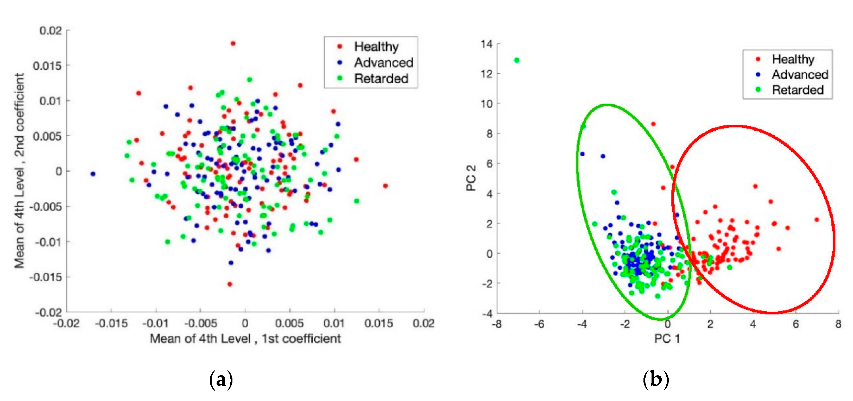
Features once extracted can be a useful input for classification, but a large number of features can often result in less accuracy and longer execution time. Therefore, feature space dimension reduction techniques become necessary. PCA is such a technique which computes the PCs commonly by singular value decomposition of a data covariance matrix. PCs are new variables constructed as a linear combination of the initial features. They are uncorrelated due to being orthogonal to each other in the Cartesian space. Taking the ignition timing variation case as an example, Figure 5a shows the plot between two features (the mean values of the first and second sets of coefficients) for different conditions. It can be seen that differentiation among the three conditions is imperceptible. After applying PCA, the first two PCs are plotted as shown in Figure 5b for the three conditions, and it shows that the healthy and the retarded conditions are more distinguishable from each other.

Figure 5. Feature space of: (a) an existing feature set (Mean of Coefficient 1 vs. Mean of Coefficient 2); and (b) the first two principle components (PC1 vs. PC2).

The critical aspect of the PCA is choosing the number of PCs to be retained. This can be done by ranking the features in their order of significance. Ranking is done based on the eigenvalues. The percentage of total variance of each PC is calculated. For all datasets, the threshold of the total percentage of variance was chosen to be 99% for determining the optimal number of retained PCs.

3.4. Classification Algorithm Selection

Classification algorithms are widely used in condition monitoring to differentiate between healthy and faulty signals. Here, six standard classifier algorithms were considered: decision tree, Naïve Bayes, k-Nearest Neighbors (kNN), Support Vector Machine (SVM), Discriminant analysis and Ensemble classification. These classifiers are explained briefly as follow; readers can be directed to the references for further details.

• Decision tree performs classification by creating a tree based on attributes of data. It uses hierarchical structures to find patterns in data for the purpose of constructing decision-making rules, to estimate the relationship between independent and dependent variables [38]. The hyperparameters for optimization here are minimum leaf size, maximum number of split and the split criteria, which further includes the Gini’s diversity index, the twoing rule or the maximum deviance reduction.
• Naïve Bayes is a type of supervised learning algorithm based on the Bayes theorem, which classifies new data using the conditional probability to predict the outcome of an occurrence [39]. The hyperparameters used for optimization here are the distribution type, the window width and the kernel type. The distributions used include Gaussian, multivariate multinomial, multinomial and kernel. The kernel smoothing window width is given by
  $$f\left(x\right)=\frac{{{\displaystyle \sum }}_{j=1}^{n}K\left\{\frac{x-X_i}{h}\right\}}{nh}$$
  where K is the kernel function.
• kNN algorithm is a supervised learning method which uses non-parametric method for classification. It classifies new data by calculating the distance of this data instance with the existing data instances, and then it selects the closest k instances for classification [40]. The hyperparameters used for optimizing the kNN include the distance measure, the number of neighbors and the distance weights.
• SVM is a type of supervised learning algorithm, which achieves classification by creating a hyperplane with the maximum margin that separates two classes [41]. The hyperparameters used for optimizing the SVM are the Box constraint, the kernel function, the kernel scale and the polynomial order. Box constraint controls the penalty imposed on observations that lie outside the margin and helps prevent overfitting. The kernel functions used for optimization include Gaussian, linear and polynomial.
• Discriminant analysis is an effective subspace technique which also uses Bayes theorem similar to Naïve Bayes. The Bayesian rule divides the data space into disjoint regions that represent all the classes using the probability densities [42]. The hyperparameters for optimization here are Delta, Gamma and the type of discriminate. Delta is the amount of regularization to be applied when estimating the covariance matrix and Gamma is the linear coefficient threshold. The types of discriminates used include linear and quadratic.
• Ensemble classifier is relatively new classification technique which has gained popularity in the recent years. It uses different classification techniques to improve the model accuracy [43]. The hyperparameters for optimization here are the classification method, number of learning cycles, learn rate, etc. There are several methods used for multiclassification problems such adaptive boosting, linear programming boosting and random under-sampling boosting.

The standard model is obtained by running the data in each classifier using default parameters and finding the best fit model for each fault case. The best fit classifier and default parameters used by the standard model for each fault case are listed in Table 4.

Table 4. Optimal model selection for Model 1—using a standard model.

Engine Miss-Fire		Ignition Timing Variation		AFR Variation
Hyperparameter	Selection	Hyperparameter	Selection	Hyperparameter	Selection
Classification Model	Naïve Bayes	Classification Model	Ensemble	Classification Model	kNN
Kernel	Gaussian	Classifiers	Discriminant Analysis	No. of Neighbors	10
				Distance metrics	Euclidean

Then, the best fit algorithm along with its optimal hyperparameters are determined through a process using Bayesian optimization. It operates by the assumption that the unknown objective function is with samples from a Gaussian process and this achieves a posterior distribution of the samples by running different learning algorithm experiments with different hyperparameters. The hyperparameter of the next model is selected by optimizing the expected improvement compared with the current result. This has been proven to be efficient in the required number and time of function evaluations to reach the global optimum for numerous multimodal functions [29,30]. The trained model was validated by using a five-fold cross-validation. The maximum number of iterations was set to be 180. The best fit classifier and its optimal parameters for each fault case are listed in Table 5 for Model 2 and Table 6 for Model 3 (with the addition of PCA for feature dimensionality reduction).

Table 5. Optimal parameters for Model 2—using Bayesian optimization.

Engine Miss-Fire		Ignition Timing Variation		AFR Variation
Hyperparameter	Selection	Hyperparameter	Selection	Hyperparameter	Selection
Classification Model	Naïve Bayes	Classification Model	Ensemble	Classification Model	Discrim. Analysis
Kernel	Gaussian	Classifiers	Decision Trees	Discrim. Type	Linear
Width	0.0094	Split criteria	Gini’s Diversity Index	Delta	0.00010747
				Gamma	0.038118

Table 6. Optimal parameters for Model 3—using PCA in addition to Bayesian optimization.

Engine Miss-Fire		Ignition Timing Variation		AFR Variation
Hyperparameter	Selection	Hyperparameter	Selection	Hyperparameter	Selection
Classification Model	kNN	Classification Model	Ensemble	Classification Model	SVM
No. of Neighbors	1	Classifiers	Decision Trees	Coding	one vs. all
Distance metrics	Correlation	Split criteria	Gini’s Diversity Index	Box constraint	0.483
				Kernel Function	Linear

3.5. Model Evaluation

The extracted feature matrix is then fed into the three models described in Figure 4, and the performance of each model is evaluated using the metrics listed in Table 7. True Positive (TP) are the data points which are accurately classified as faulty data and False Positive (FP) are the data points which are incorrectly classified as faulty data. True Negative (TN) are the data points which are accurately classified as healthy data and False Negative (FN) are the data points which are incorrectly classified as healthy data. Specificity indicates the proportion of negatives that are correctly identified, whereas precision indicates the proportion of positive that are correctly identified. These metrics along with the most commonly used accuracy measure are all very important in examining a model’s performance.

Table 7. Model evaluation metrics.

Metric	Formula Used
Accuracy	$\frac{\mathrm{TP}+\mathrm{TN}}{\mathrm{TP}+\mathrm{FP}+\mathrm{TN}+\mathrm{FN}}$
Precision	$\frac{\mathrm{TP}}{\mathrm{TP}+\mathrm{FP}}$
Sensitivity	$\frac{\mathrm{TP}}{\mathrm{TP}+\mathrm{FN}}$
Specificity	$\frac{\mathrm{TN}}{\mathrm{TP}+\mathrm{TN}}$
F1 Score	$\frac{2\mathrm{TP}}{2\mathrm{TP}+\mathrm{FP}+\mathrm{FN}}$

4. Results

The total dataset was divided into a training dataset and a test dataset in a ratio of 80:20. A five-fold cross-validation was applied to validate the trained models.

4.1. Model 1—Standard Classification Approach

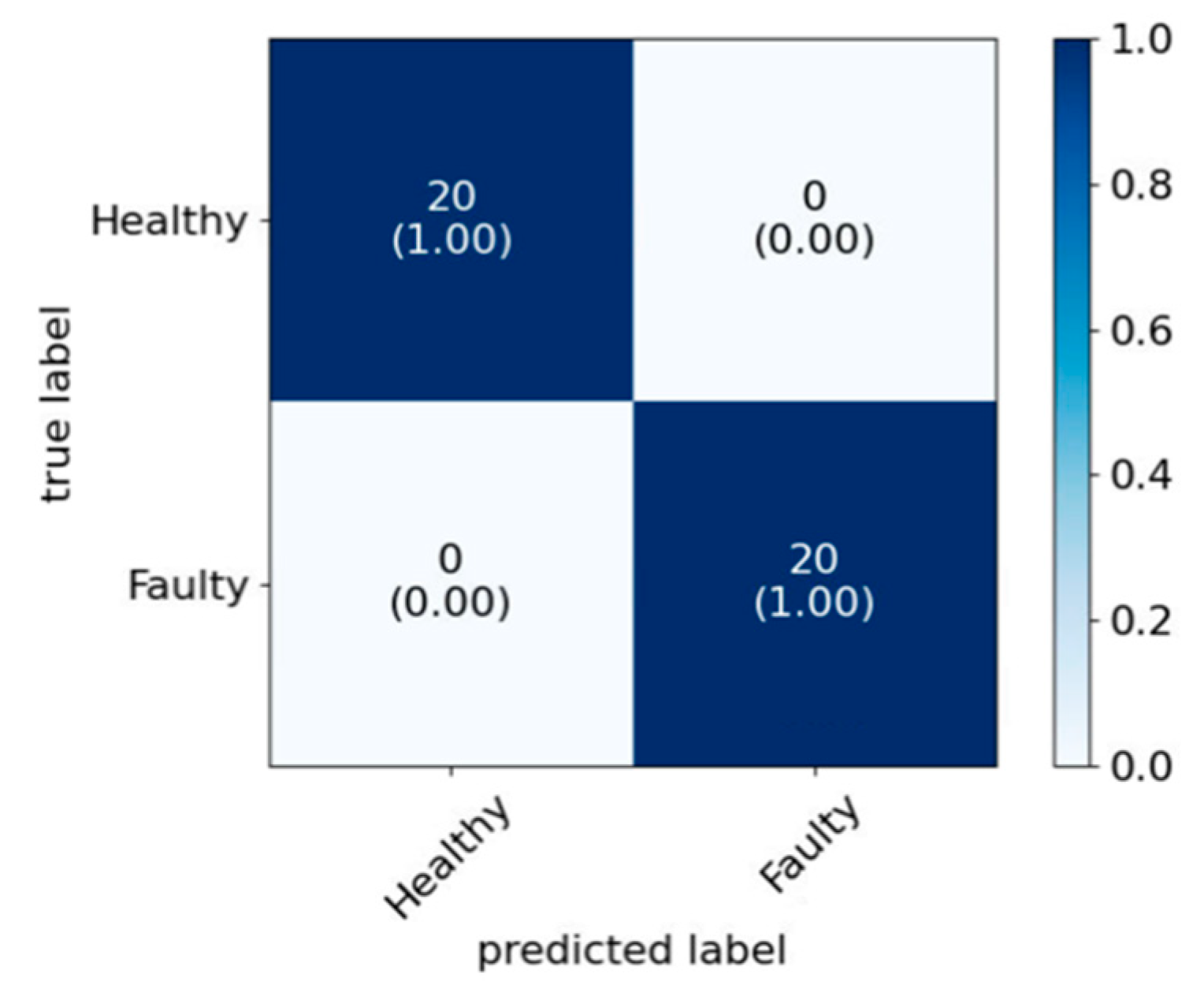
The confusion matrixes for Model 1 are presented in Figure 6, Figure 7 and Figure 8 for the three experimental cases. From the confusion matrixes, it is evident that Model 1 can be applicable in classifying fault in the case of engine misfire, where the FN and FP are negligible. However, it is seen that, for the ignition timing variation and AFR variation data, Model 1 is comparatively less successful due to higher operational complexity.

Figure 6. Model 1—confusion matrix and for engine misfire data.

Figure 7. Model 1—confusion matrix for ignition timing variation data.

Figure 8. Model 1—confusion matrix for AFR variation data.

4.2. Model 2—Bayesian Optimization for Combined Model and Hyperparameters Selection

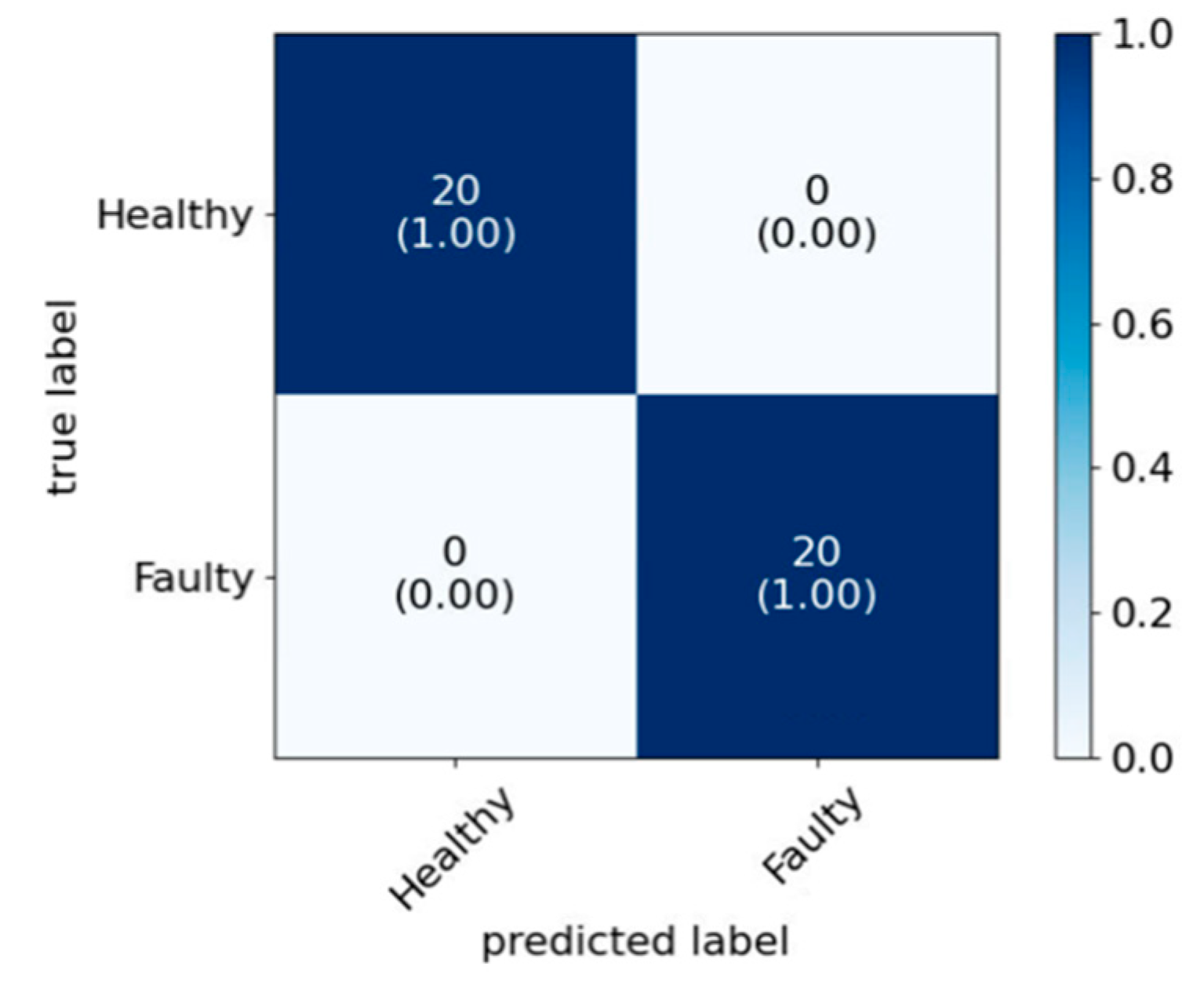
The confusion matrixes for Model 2 are presented in Figure 9, Figure 10 and Figure 11 for the three experimental cases. From the confusion matrixes, it can be seen that there is a significant improvement in FN, FP, TP and TN, compared to those of Model 1 (the standard model).

Figure 9. Model 2—confusion matrix for engine misfire data.

Figure 10. Model 2—confusion matrix for ignition timing variation data.

Figure 11. Model 2—confusion matrix for AFR variation data.

4.3. Model 3—PCA with Bayesian Optimization

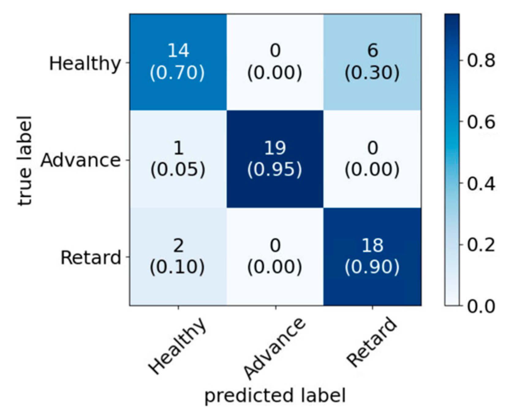
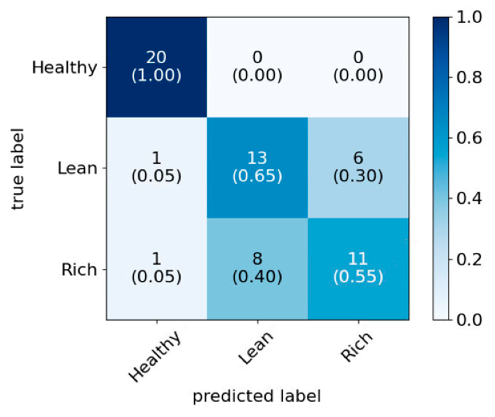
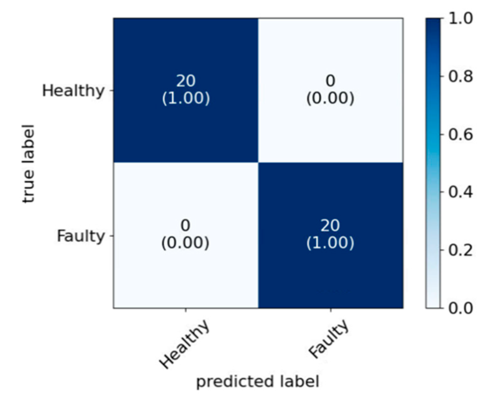
The confusion matrixes for Model 3 are presented in Figure 12, Figure 13 and Figure 14 for the three experimental cases. From the confusion matrixes, it is also seen that there is a significant improvement in FN, FP, TP and TN, compared to those of the standard model, but similar level to those of Model 2, even though the feature dimension has been reduced significantly.

Figure 12. Model 3—confusion matrix for engine misfire data.

Figure 13. Model 3—confusion matrix for ignition timing variation data.

Figure 14. Model 3—confusion matrix for AFR variation data.

4.4. Discussion

The objective of this research was to determine the faulty engine signal in real-time with acceptable classification accuracy for different fault conditions. Table 8 shows the model evaluation metrics for the three models using the equations in Table 7.

Table 8. Model evaluation metrics (%).

	Model 1			Model 2			Model 3
	EM 1	IGV 2	AFRV 3	EM	IGV	AFRV	EM	IGV	AFRV
Accuracy	100	80	68	100	85	73	100	83	72
Precision	100	83	96	100	86	100	100	88	100
Sensitivity	100	88	55	100	93	60	100	88	58
Specificity	100	65	95	100	70	100	100	75	100
F1 score	100	85	70	100	89	75	100	88	73

¹ Engine misfire; ² ignition timing variation; ³ AFR variation.

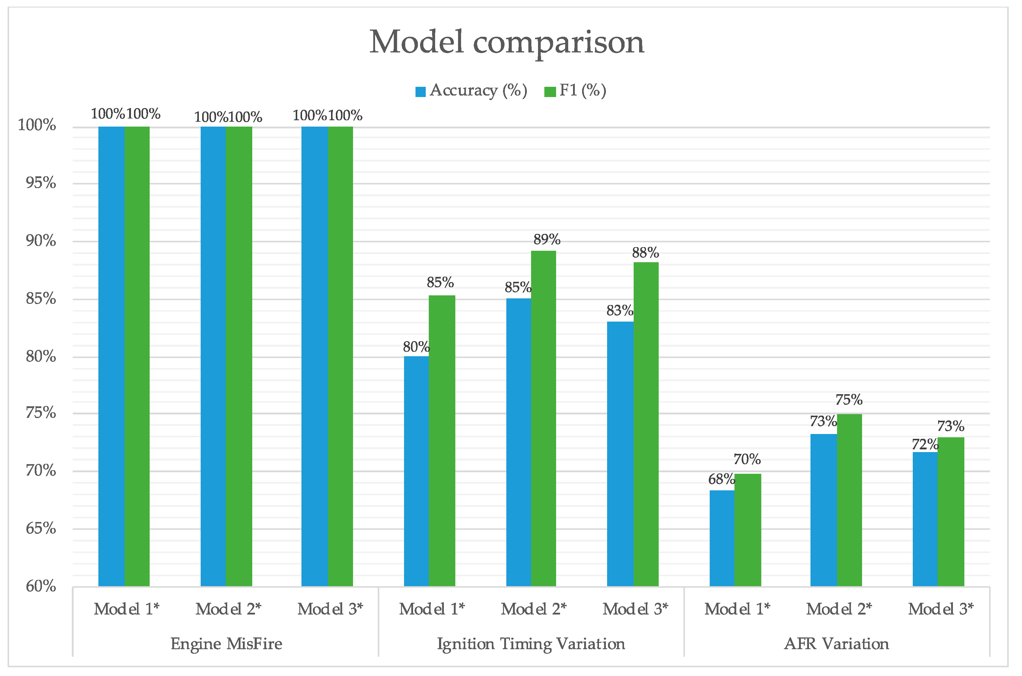
The bar chart in Figure 15 shows the improvement in accuracy and F1 score when using Bayesian optimization over the standard model for all three fault conditions. In engine misfire condition, all three models show the same performance, as classification is apparent in a simple fault scenario, but for the other two more complex faults there is a 5% increase in accuracy by implementation of Bayesian optimized model, and a 3–4% increase in accuracy by implementation of PCA with Bayesian optimized model, compared to the standard model. On the other hand, there is a less significant change in the accuracy and F1 score when comparing Model 2 and Model 3, even though the feature dimensionality has been considerably reduced by using PCA in Model 3. This effect can be demonstrated by comparing their evaluation time.

Figure 15. Accuracy and F1 score of the three models with three fault conditions. * Model 1, standard classification; * Model 2, Bayesian optimization; * Model 3, PCA with Bayesian optimization.

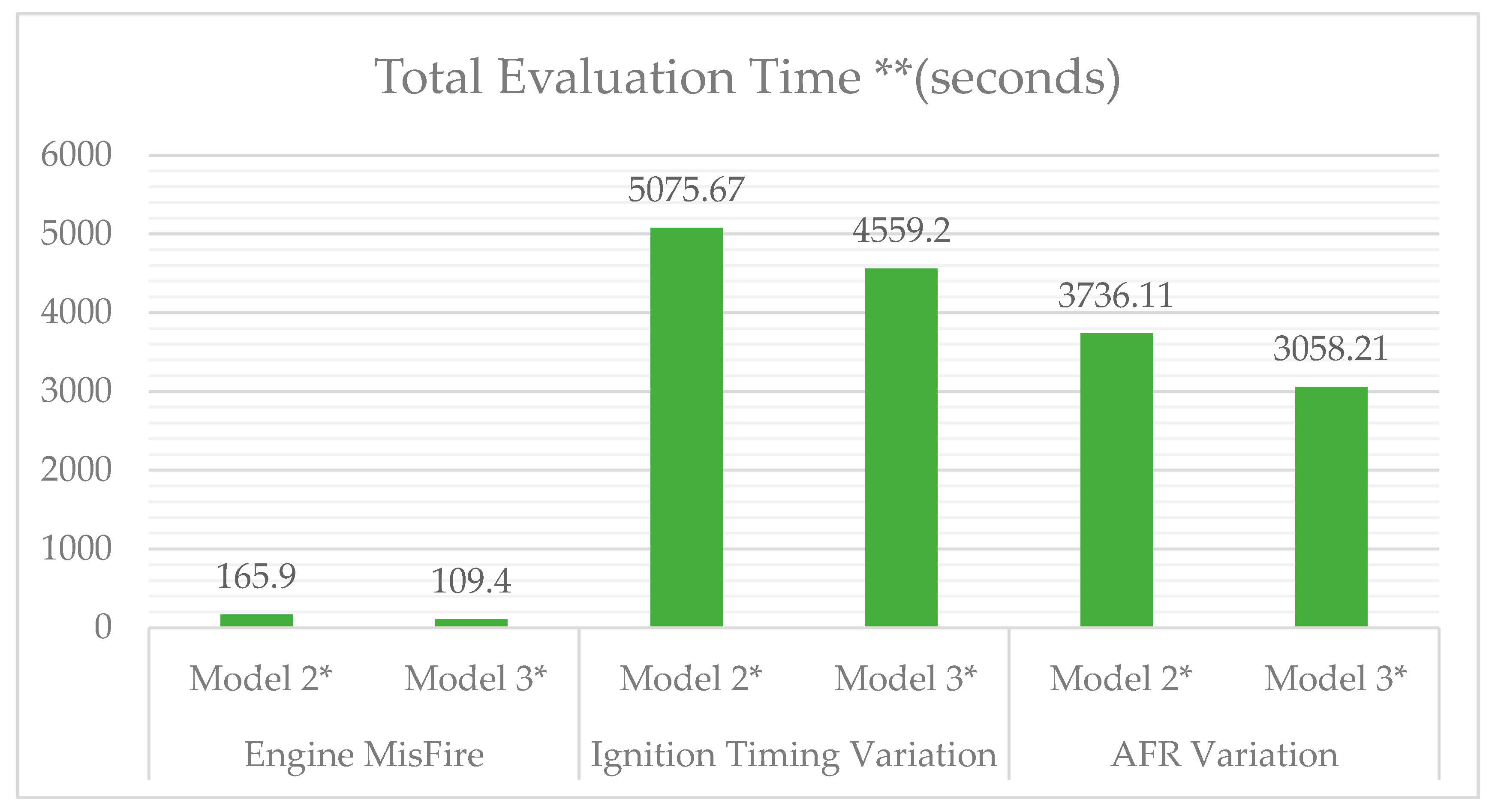
The comparison the total training and testing time between Model 2 and Model 3 in Figure 16 shows that the PCA has helped significantly lower the evaluation time by ~20% compared to the Model 2 due to its reduced feature dimensionality. Standard model is not considered in this comparison since it requires manual effort and time to implement the best fit model, whereas the other two models are automated processes which require minimal human intervention.

Figure 16. Evaluation time comparison for the models with three fault conditions. * Model 2, Bayesian optimization; * Model 3, PCA with Bayesian optimization. ** Computations were performed on a 2.7 GHz Intel dual Core i5 MacBook pro and programming was done in MATLAB R20.

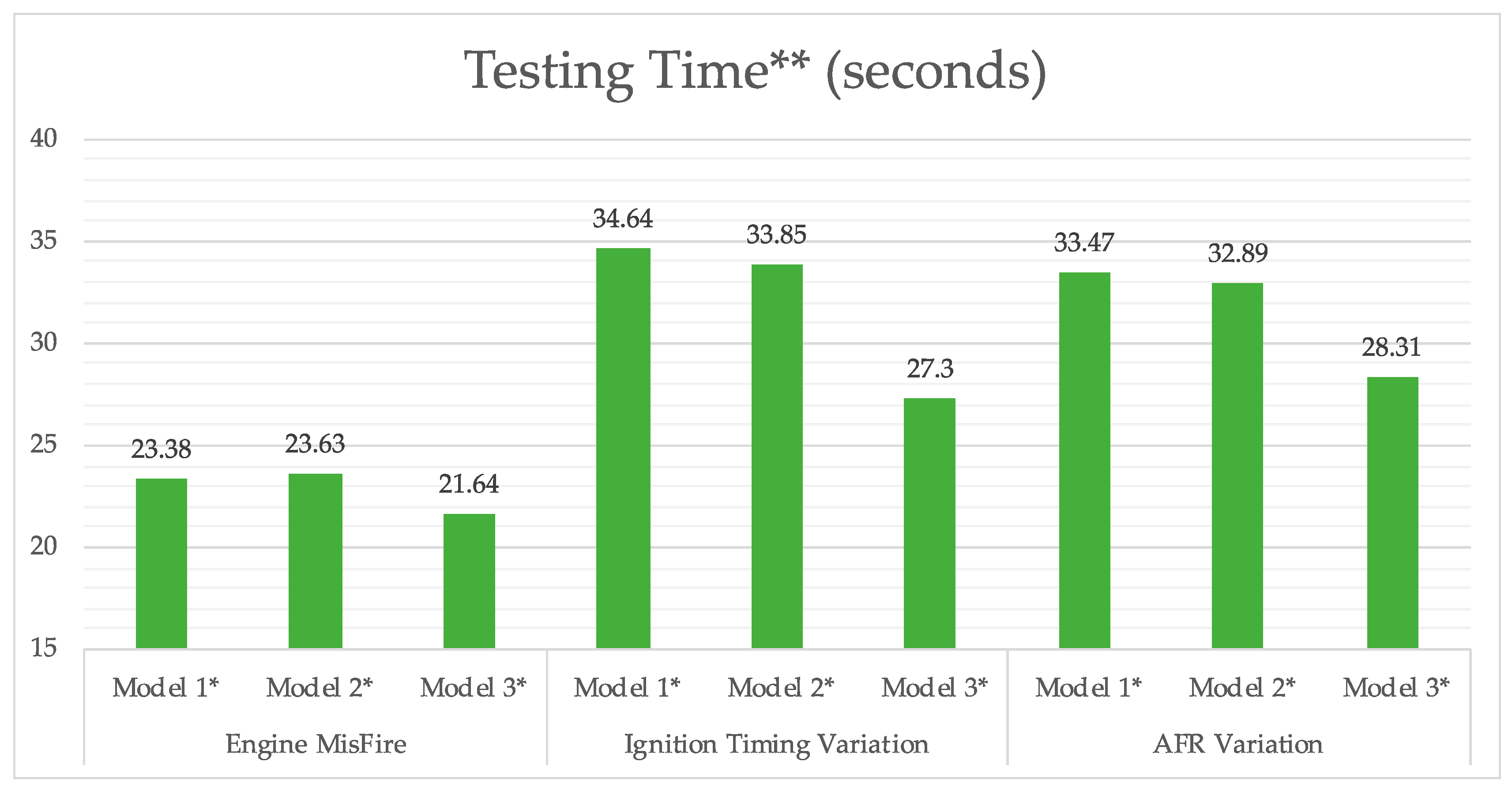
Figure 17 shows that using PCA reduces the testing time for all fault cases by 8–19%, when compared to Model 1 and Model 2, as well due to the fact that, PCA has reduced the dimensionality of the feature matrix.

Figure 17. Testing time comparison for the models with three fault conditions. * Model 1, standard classification; * Model 2, Bayesian optimization; * Model 3, PCA with Bayesian optimization. ** Computations were performed on a 2.7 GHz Intel dual Core i5 MacBook pro and programming was done in MATLAB R20.

In summary, PCA with Bayesian optimized model is a promising and highly effective methodology with better evaluation time and classification accuracy compared to the standard model for different fault settings.

5. Conclusions

In this study, a data-driven approach based on engine acoustic signals for classification was proposed for ICE fault diagnosis. Three faulty conditions, namely engine misfire, ignition timing variation and AFR variation, were used to train and test the applicability of the approach. Three models were studied, i.e., the standard classification approach (Model 1), the Bayesian optimized model (Model 2) and the use of PCA alongside Bayesian optimization (Model 3). In all cases, WPT was used to decompose the acoustic signals, and the statistical features were extracted from the wavelet coefficients, which were then used as the input of the three classification models. The aim of the study was not only to achieve the highest accuracy, but also to reduce the computational time by eliminating redundant features. In doing so, the feature sets with reduced dimension would be more suitable for the future online implementation in real-time engine fault diagnosis applications. Both Model 2 and Model 3 achieved better accuracy and the other performance metrics than the standard model for all three faults. With similar accuracy level compared to Model 2, Model 3 achieved ~20% less combined training and testing evaluation time and 8–19% less time for testing evaluations for the fault cases. This indicates that the WPT with PCA and Bayesian optimization technique could be a promising tool for real-time acoustic engine fault diagnosis application.

In reality, there is a trade-off between the fault classification accuracy and the processing time saving, and it will depend on the industrial application and their specific requirement. For example, if the application requires high accuracy in the fault diagnosis, as a false alarm can result in excessive downtime costs, the user may prefer to select Model 2 at the expense of additional processing time. On the other hand, if, for example, some combustion faults need to be identified within a short time duration, before they lead to catastrophic component damage, then the user may consider that implementing Model 3 on fast computing electronics will be essentially beneficial for this application.

References

- Internal Combustion Engines (ICE) Counted for Over 90% of Global Car Sales in H1 2019. Available online: https://www.jato.com/internal-combustion-engines-ice-counted-for-over-90-of-global-car-sales-in-h1-2019/ (accessed on 12 August 2020).
- Heywood, J.B. Internal Combustion Engine Fundamentals; Mcgraw-Hill Education: New York, NY, USA, 2018. [Google Scholar]
- Zhang, Y.; Martinez-Garcia, M.; Kalawsky, R.S.; Latimer, A. Grey-box modelling of the swirl characteristics in gas turbine combustion system. Measurement 2020, 151, 107266. [Google Scholar] [CrossRef]
- Moosavian, A.; Najafi, G.; Ghobadian, B.; Mirsalim, M.; Jafari, S.M.; Sharghi, P. Piston scuffing fault and its identification in an IC engine by vibration analysis. Appl. Acoust. 2016, 102, 40–48. [Google Scholar] [CrossRef]
- Jiang, K.; Cao, E.; Wei, L. NOx sensor ammonia cross sensitivity estimation with adaptive unscented Kalman filter for Diesel-engine selective catalytic reduction systems. Fuel 2016, 165, 185–192. [Google Scholar] [CrossRef]
- Shao, H.; Xia, M.; Han, G.; Zhang, Y.; Wan, J. Intelligent fault diagnosis of rotor-bearing system under varying working conditions with modified transfer CNN and thermal images. IEEE Trans. Ind. Inform. 2020. [Google Scholar] [CrossRef]
- Traver, M.L.; Atkinson, R.J.; Atkinson, C.M. Neural network-based diesel engine emissions prediction using in cylinder combustion pressure. SAE Trans. 1999, 108, 1166–1180. [Google Scholar]
- Li, Z.; Yan, X.; Yuan, C.; Peng, Z. Intelligent fault diagnosis method for marine diesel engines using instantaneous angular speed. J. Mech. Sci. Technol. 2012, 26, 2413–2423. [Google Scholar] [CrossRef]
- Burdzik, R.; Konieczny, L. Application of Vibroacoustic Methods for Monitoring and Control of Comfort and Safety of Passenger Cars, Diffusion and Defect Data. In Solid State Phenomena; Trans Tech Publications Ltd.: Stafa-Zurich, Switzerland, 2014; Volume 210, pp. 20–25. [Google Scholar]
- Zhang, Y.; Martinez-Garcia, M.; Latimer, A. Selecting Optimal Features for Cross-Fleet Analysis and Fault Diagnosis of Industrial Gas Turbines; ASME Turbo Expo: Oslo, Norway, 2018. [Google Scholar]
- Herrera, J.A.G.; López, J.F.L.; Riaza, H.F.Q. Diagnostic method based on the analysis of vibration and acoustic emissions for internal combustion engines faults. In Proceedings of the 2014 XIX Symposium on Image, Signal Processing and Artificial Vision, Armenia, Colombia, 17–19 September 2014. [Google Scholar]
- Zhang, Y.; Bingham, C.; Yang, Z.; Ling, B.W.K.; Gallimore, M. Machine fault detection by signal denoising—With application to industrial gas turbines. Measurement 2014, 58, 230–240. [Google Scholar] [CrossRef]
- Zabihi-Hesari, A.; Ansari-Rad, S.; Shirazi, F.A.; Ayati, M. Fault detection and diagnosis of a 12-cylinder trainset diesel engine based on vibration signature analysis and neural network. Part C J. Mech. Eng. Sci. 2014, 233, 1910–1923. [Google Scholar] [CrossRef]
- Albarbar, A. An investigation into diesel engine air-borne acoustics using continuous wavelet transform. J. Mech. Sci. Technol. 2013, 27, 2599–2604. [Google Scholar] [CrossRef]
- Nidadavolu, S.V.P.S.; Yadav, S.K.; Kalra, P.K. Condition monitoring of Internal Combustion engines using empirical mode decomposition and Morlet wavelet. In Proceedings of the 6th International Symposium on Image and Signal Processing and Analysis, Salzburg, Austria, 16–18 September 2009; pp. 65–72. [Google Scholar]
- Muralidharan, V.; Sugumaran, V. Feature extraction using wavelets and classification through decision tree algorithm for fault diagnosis of mono-block centrifugal pump. Measurement 2013, 46, 353–359. [Google Scholar] [CrossRef]
- Plaza, E.G.; López, P.J. NApplication of the wavelet packet transform to vibration signals for surface roughness monitoring in CNC turning operations. Mech. Syst. Signal. Process. 2018, 98, 902–919. [Google Scholar] [CrossRef]
- Figlus, T.; Liščák, Š.; Wilk, A.; Łazarz, B. Condition monitoring of engine timing system by using wavelet packet decomposition of an acoustic signal. J. Mech. Sci. Technol. 2014, 28, 1663–1671. [Google Scholar] [CrossRef]
- Liu, C.; Gao, Q.; Jin, Y.; Yang, W. Application of wavelet packet transform in the knock detection of gasoline engines. In Proceedings of the International Conference on Image Analysis and Signal Processing, Zhejiang, China, 9–11 April 2010; pp. 686–690. [Google Scholar]
- Moosavian, A.; Jafari, S.M.; Khazaee, M.; Ahmadi, H. A comparison between ANN, SVM and least squares SVM: Application in multi-fault diagnosis of rolling element bearing. Int. J. Acoust. Vib. 2018, 23, 432–440. [Google Scholar]
- Gangsar, P.; Tiwari, R. A support vector machine based fault diagnostics of Induction motors for practical situation of multi-sensor limited data case. Measurement 2019, 135, 694–711. [Google Scholar] [CrossRef]
- Martinez-Garcia, M.; Zhang, Y.; Suzuki, K.; Zhang, Y.D. Deep recurrent entropy adaptive model for system reliability monitoring. IEEE Trans. Ind. Inform. 2020. [Google Scholar] [CrossRef]
- Moosavian, A.; Ahmadi, H.; Tabatabaeefar, A.; Khazaee, M. Comparison of two classifiers: K-nearest neighbor and artificial neural network, for fault diagnosis on a main engine journal-bearing. Shock. Vib. 2013, 20, 263–272. [Google Scholar] [CrossRef]
- Nishat Toma, R.; Kim, J.-M. Bearing fault classification of induction motors using discrete wavelet transform and ensemble machine learning algorithms. Appl. Sci. 2020, 10, 5251. [Google Scholar] [CrossRef]
- Xia, Y.; Liu, C.; Li, Y.; Liu, N. A boosted decision tree approach using Bayesian hyper-parameter optimization for credit scoring. Expert Syst. Appl. 2017, 75, 225–241. [Google Scholar] [CrossRef]
- Vilalta, R.; Drissi, Y. A perspective view and survey of meta-learning. Artif. Intell. Rev. 2002, 18, 77–95. [Google Scholar] [CrossRef]
- Jones, D.R. A taxonomy of global optimization methods based on response surfaces. J. Glob. Optim. 2001, 21, 345–383. [Google Scholar] [CrossRef]
- Mockus, J.; Tiesis, V.; Zilinskas, A. The application of Bayesian methods for seeking the extremum. Towards Glob. Optim. 1978, 2, 117–129. [Google Scholar]
- Adam, D.B. Convergence rates of efficient global optimization algorithms. J. Mach. Learn. Res. 2011, 12, 2879–2904. [Google Scholar]
- Niranjan Srinivas, N.; Andreas, K.; Sham, K.; Matthias, S. Gaussian process optimization in the bandit setting: No regret and experimental design. In Proceedings of the 27th International Conference on Machine Learning, Haifa, Israel, 21–24 June 2010. [Google Scholar]
- Thornton, C.; Hutter, F.; Hoos, H.H.; Leyton-Brown, K. Auto-WEKA: Combined selection and hyperparameter optimization of classification algorithms. Proc. Knowl. Disc. Data Mining 2013, 847–855. [Google Scholar] [CrossRef]
- Jafarian, K.; Darjani, M.; Honarkar, Z. Vibration analysis for fault detection of automobile engine using PCA technique. In Proceedings of the 4th International Conference on Control, Instrumentation, and Automation (ICCIA), Qazvin, Iran, 27–28 January 2016; pp. 372–376. [Google Scholar]
- Jolliffe, I.T. Principal Component Analysis, 2nd ed.; Springer: New York, NY, USA, 2002. [Google Scholar]
- Kabiri, P.; Makinezhad, A. Using PCA in acoustic emission condition monitoring to detect faults in an automobile engine. In Proceedings of the 29th European Conference on Acoustic Emission Testing (EWGAE2010), Vienna, Austria, 8–10 September 2010; pp. 8–10. [Google Scholar]
- Zhang, Q.; Hao, Z.; Zheng, X.; Yang, W.Y.; Mao, J. Mechanism and optimization of fuel injection parameters on combustion noise of DI diesel engine. J. Cent. South Univ. 2016, 23, 379–393. [Google Scholar] [CrossRef]
- Anderton, D. Relation between combustion system and engine noise. SAE Trans. 1979, 88, 1000–1014. [Google Scholar]
- Chen, J.L.; Pan, J.; Li, Z.P.; Zi, Y.Y.; Chen, X.F. Generator bearing fault diagnosis for wind turbine via empirical wavelet transform using measured vibration signals. Renew. Energy 2016, 89, 80–92. [Google Scholar] [CrossRef]
- Breiman, L.; Friedman, J.; Stone, C.J.; Olshen, R.A. Classification and Regression Trees; CRC Press: Boca Raton, FL, USA, 1984. [Google Scholar]
- Kumar, H.; Ranjit Kumar, T.A.; Amarnath, M.; Sugumaran, V. Fault Diagnosis of Bearings through Vibration Signal Using Bayes Classifiers. Int. J. Comput. Aided Eng. Technol. 2014, 6, 14–28. [Google Scholar] [CrossRef]
- VanderPlas, J. Python Data Science Handbook; O’Reilly Media, Inc.: Sevastopol, CA, USA, 2016. [Google Scholar]
- Kotsiantis, S. Supervised Machine Learning: A Review of Classification Techniques. Informatica 2007, 31, 249–269. [Google Scholar]
- Bandos, T.V.; Bruzzone, L.; Camps-Valls, G. Classification of Hyperspectral Images with Regularized Linear Discriminant Analysis. IEEE Trans. Geosci. Remote. Sens. 2009, 47, 862–873. [Google Scholar] [CrossRef]
- Maritnez-Alvarez, F.; Troncoso, A.; Asencio-Cortes, G.; Riquelme, J.C. A survey on data mining techniquesapplied to electricity-related time series forecasting. Energies 2015, 8, 13162–13193. [Google Scholar] [CrossRef]
© 2020 by the authors. Licensee MDPI, Basel, Switzerland. This article is an open access article distributed under the terms and conditions of the Creative Commons Attribution (CC BY) license (http://creativecommons.org/licenses/by/4.0/).