An e-Learning Toolbox Based on Rule-Based Fuzzy Approaches


Abstract
1. Introduction
2. Materials and Methods
2.1. Logical Rules Extraction from FIR Models: LR-FIR
- Basic compaction. The main goal of this step is to transform the pattern rule base, into a reduced set of rules. It consist on an iterative step that evaluates one at a time, all of the rules, and each of their premises in the pattern rule base. A specific subset of rules can be transformed in the form of a compacted rule when all premises but one, as well as the consequence share the same values. If the subset contains all legal values, all these rules can be replaced by a single rule that has a value of −1 in that premise, and if no conflicts exists the compacted rule is accepted. Conflicts occur when the extended rules have the same values in all its premises, but different values in the consequence. The reduced set of rules includes all the rules compacted in previous iterations and those that cannot be compacted in this step.
- Improved compaction. This step extends the pattern rule base to cases that had not been previously used to build the model. In this compaction, a consistent minimal ratio of the legal values should be present in the candidate subset in order to compact it in the form of a single rule. In this case, assumed beliefs are incorporated to the set of compacted rules to some extent, not compromising the model previously identified by FIR. The obtained set of rules is subjected to a number of refinement steps: removal of duplicate rules and conflicting rules, unification of similar rules, etc. For a deeper insight into LR-FIR, the reader is referred to [34].
2.2. Causal Relevance Approaches: CR-FIR
3. The Toolbox
3.1. Modeler
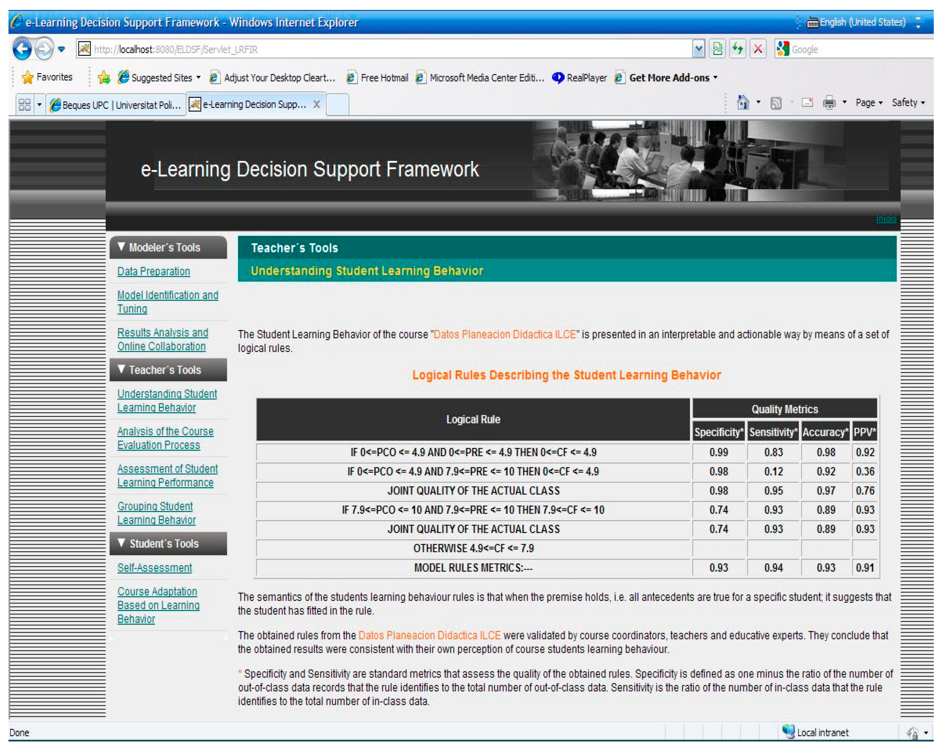
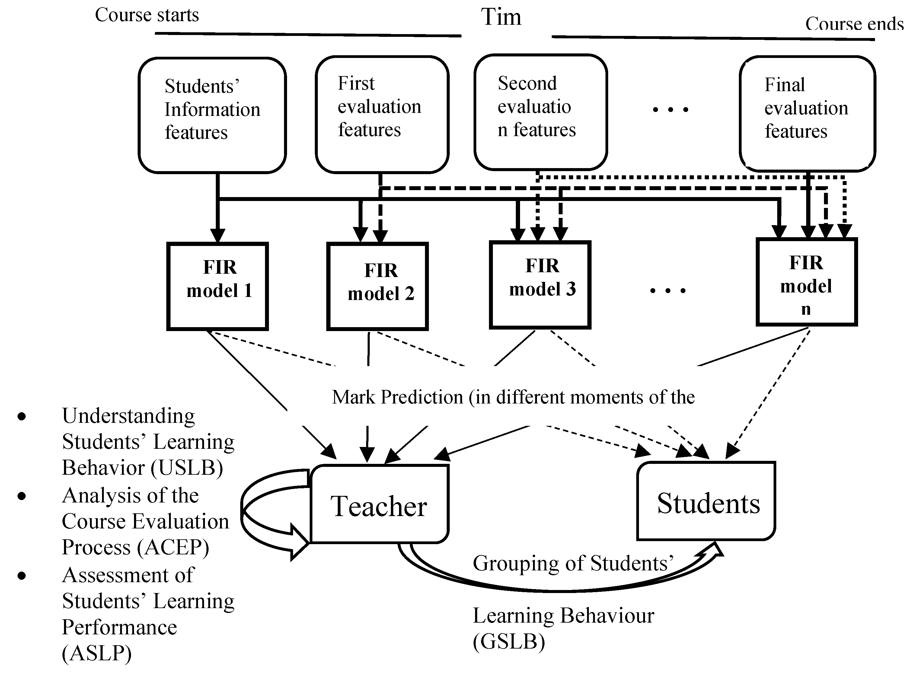
3.2. Teacher
3.3. Student
4. Results and Discussion
4.1. Didactic Planning Course
4.1.1. Time 1 Model
4.1.2. Time 2 Model
4.1.3. Time 3 Model
4.1.4. Time 4 Model
4.1.5. Using the Toolbox in the Next Course
4.2. Introductory Course
4.2.1. Time 1 Model
4.2.2. Time 2 Model
4.2.3. Time 3 Model
4.2.4. Time 4 Model
4.2.5. Using the Toolbox in the Next Course
5. Conclusions
Author Contributions
Funding
Acknowledgments
Conflicts of Interest
References
- Arkorful, V.; Abaidoo, N. The role of e-learning, advantages and disadvantages of its adoption in higher education. Int. J. Instr. Technol. Distance Learn. 2015, 12, 29–42. [Google Scholar]
- Dwivedi, S.K.; Rawat, B. An Architecture for Recommendation of Courses in e-Learning. Int. J. Inf. Technol. Comput. Sci. 2017, 4, 39–47. [Google Scholar] [CrossRef]
- Vellido, A.; Castro, F.; Nebot, A. Clustering educational data. In Handbook of Educational Data Mining; Chapman & Hall/CRC Press: London, UK, 2011; pp. 75–92. ISBN 9781439804575. [Google Scholar]
- Abu-Naser, S.; Ahmed, A.; Al-Masri, N.; Deeb, A.; Moshtaha, E.; Abu-Lamdy, M. An Intelligent Tutoring System for Learning Java Objects. Int. J. Artif. Intell. Appl. 2011, 2, 68–77. [Google Scholar] [CrossRef]
- Zorrilla, M.E.; Garcia, D.; Álvarez, E. A decision support system to improve e-learning environments. In Proceedings of the 2010 EDBT/ICDT Workshops, Lausanne, Switzerland, 22–26 March 2010; pp. 1–8. [Google Scholar]
- Hegazi, M.O.; Abugroon, M.A. The State of the Art on Educational Data Mining in Higher Education. Int. J. Comput. Trends Technol. 2016, 31, 46–56. [Google Scholar] [CrossRef]
- Peña Ayala, A. Educational Data Mining: A survey and Data Mining-based analysis. Expert Syst. Appl. 2014, 41, 1432–1462. [Google Scholar] [CrossRef]
- Santos, O.C.; Barrera, C.; Boticario, J.G. An Overview of aLFanet: An Adaptive iLMS based on standards. In Adaptive Hypermedia and Adaptive Web-Based Systems; De Bra, P.M.E., Nejdl, W., Eds.; Lecture Notes in Computer Science; Springer: Berlin/Heidelberg, Germany, 2004; Volume 3137. [Google Scholar]
- aLFanet. Available online: http://adenu.ia.uned.es/alfanet/ (accessed on 13 May 2020).
- Romero, C.; Ventura, S.; Delgado, J.A.; De Bra, P. Personalized Links Recommendation Based on Data Mining in Adaptive Educational Hypermedia Systems. In Proceedings of the second European Conference on Technology Enhanced Learning, EC-TEL, Crete, Greece, 17–20 September 2007; Springer LNCS: Berlin/Heidelberg, Germany, 2007. [Google Scholar]
- AHA. Available online: http://aha.win.tue.nl (accessed on 13 May 2020).
- Kortemeyer, G. LON-CAPA–An Open-Source Learning Content Management and Assessment System. In Proceedings of the ED-MEDIA -World Conference on Educational Multimedia, Hypermedia & Telecommunications, Honolulu, HI, USA, 22 June 2009; pp. 1515–1520. [Google Scholar]
- LON-CAPA. Available online: https:/loncapa.msu.edu/adm/login (accessed on 13 May 2020).
- ATutor. Available online: https://atutor.github.io/ (accessed on 13 May 2020).
- LExIKON. Available online: https://www.dfki.de/web/forschung/edtec/ (accessed on 13 May 2020).
- Blackboard. Available online: http://www.blackboard.com/index.html (accessed on 13 May 2020).
- Weber, G.; Brusilovsky, P. ELM-ART—An Interactive and Intelligent Web-Based Electronic Textbook. Int. J. Artif. Intell. Educ. 2016, 26, 72–81. [Google Scholar] [CrossRef]
- ELM-ART. Available online: http://art2.ph-freiburg.de/Lisp-Course (accessed on 13 May 2020).
- Moodle, Learning Analytics. Available online: https://moodle.com/ (accessed on 13 May 2020).
- Liu, D.Y.T.; Froissard, J.C.; Richards, D.; Atif, A. An enhanced learning analytics plugin for Moodle: Student engagement and personalised intervention. In Proceedings of the ASCILITE 2015–Australasian Society for Computers in Learning and Tertiary Education, Conference Proceedings, Perth, Australia, 30 November–3 December 2019; pp. 180–189. [Google Scholar]
- Akcapinar, G.; Bayasit, A. MoodleMiner: Data Mining Analysis Tool for Moodle Learning Management System. Elem. Educ. Online 2019, 18, 406–415. [Google Scholar] [CrossRef]
- GISMO. Available online: http://gismo.sourceforge.net (accessed on 10 September 2020).
- Lu, O.H.T.; Huang, A.Y.Q.; Huang, J.C.H.; Lin, A.J.Q.; Ogata, H.; Yang, S.J.H. Applying Learning Analytics for the Early Prediction of Students’ Academic Performance in Blended Learning. Educ. Technol. Soc. 2018, 21, 220–232. [Google Scholar]
- Hussain, S.; Dahan, N.A.; Ba-Alwi, F.M.; Ribata, N. Educational Data Mining and Analysis of Students’ Academic Performance Using WEKA. Indones. J. Electr. Eng. Comput. Sci. 2018, 9, 447–459. [Google Scholar] [CrossRef]
- WEKA. Available online: https://www.cs.waikato.ac.nz/ml/weka/ (accessed on 13 September 2020).
- Juhanak, L.; Zounek, J.; Rohlikova, L. Using process mining to analyze students’ quiz-taking behavior patterns in a learning management system. Comput. Hum. Behav. 2019, 92, 496–506. [Google Scholar] [CrossRef]
- Almasri, A.; Celebi, E.; Alkhawaldeh, R.S. EMT: Ensemble Meta-Based Tree Model for Predicting Student Performance. Sci. Program. Hindawi 2019, 2019, 3610248. [Google Scholar] [CrossRef]
- Aung, T.H.; Kham, N.S.M. Cloud Based Teacher’s Assessment Data in Educational Data Mining. In Proceedings of the 9th International Workshop on Computer Science and Engineering, WCSE, Hong Kong, China, 15–17 June 2019; pp. 159–164. [Google Scholar]
- Jayapradha, J.; Kumar, K.J.J.; Deka, B. Educational Data Classification and prediction using Data Mining Algorithms. Int. J. Recent Technol. Eng. 2019, 8, 8674–8678. [Google Scholar]
- Abubakar, Y.; Bahiah, N.; Ahmad, H. Prediction of Students’ Performance in E-Learning Environment Using Random Forest. Int. J. Innov. Comput. 2016, 7, 1–5. [Google Scholar]
- Klir, G.; Elias, D. Architecture of Systems Problem Solving, 2nd ed.; Plenum Press: New York, NY, USA, 2002. [Google Scholar]
- Nebot, A.; Mugica, F. Fuzzy Inductive Reasoning: A consolidated approach to data-driven construction of complex dynamical systems. Int. J. Gen. Syst. 2012, 41, 645–665. [Google Scholar] [CrossRef]
- Vellido, A.; Castro, F.; Etchells, T.A.; Nebot, A.; Mugica, F. Data Mining of Virtual Campus Data. In Evolution of Teaching and Learning Paradigms in Intelligent Environment. Studies in Computational Intelligence; Jain, L.C., Tedman, R.A., Tedman, D.K., Eds.; Springer: Berlin/Heidelberg, Germany, 2007; p. 62. [Google Scholar]
- Castro, F.; Nebot, A.; Múgica, F. On the extraction of decision support rules from fuzzy predictive models. Appl. Soft Comput. 2011, 11, 3463–3475. [Google Scholar] [CrossRef]
- Nebot, A.; Mugica, F.; Castro, F. Causal Relevance to Improve the Prediction Accuracy of Dynamical Systems using Inductive Reasoning. Int. J. Gen. Syst. 2009, 38, 331–358. [Google Scholar] [CrossRef]
- Müller, S. JMatLink Library. Available online: http://jmatlink.sourceforge.net/ (accessed on 28 September 2020).
- ILCE. Available online: http://cecte.ilce.edu.mx/ (accessed on 13 May 2020).


| Feature | Type | Description |
|---|---|---|
| AGE | Integer | Age of the student |
| EXP | Integer | Area of expertise of the student (1—mathematics, 2—chemistry, 3—Mexican history, etc.) |
| G | Integer | Student’s gender (1—male, 2—female) |
| STD | Integer | Level of studies (1—undergraduate, 2—graduate, 3—master, 4—Ph.D.) |
| POS | Integer | Position of the student as a teacher in his/her school (1—assistant, 2—associate, 3—permanent, etc.) |
| Float | Average mark obtained by the student in the activities sent by e-mail | |
| COEV | Float | Average mark of the co-evaluation performed by the student of the class plan of other students |
| F | Float | Average mark of the student’s forum participation (referring to topics related to the course) |
| FCP | Float | Average mark of the forum class plan (referring to topics related to the class plan exclusively) |
| FC | Float | Average mark obtained by the student in his/her final class plan |
| IC | Bool. | Initial class plan (delivered, not delivered) |
| ER | Float | Average mark obtained by the student in the experience report. In this report the student evaluates his/her learning process and describes the main concepts learned |
| BR | Float | Average mark of the work (activities) performed in the branch |
| MARK | Float | Final mark obtained by the student in the course |
| Analysis of the Course Evaluation Process (ACEP) Relative Relevance of the FIR Model Features: EXP = 0.48; G = 0.52 | |||
| Understanding Students’ Learning Behavior (USLB) | |||
| Rules | Sens. | Spec. | Acc. |
| if EXP is [Companies management, Computer sciences, Mexican history] and G is men then MARK is Fai if EXP is [Spanish reading and writing] and G is women then MARK is Fail | 0.05 | 0.91 | 0.78 |
| if EXP is [Computer sciences, Mexican history, Ethics and values] and G is women then MARK is Excellent | 0.57 | 0.54 | 0.56 |
| otherwise MARK is Pass | 0.38 | 0.60 | 0.54 |
| Macro-average precision: 0.34; Micro-average precision: 0.44 | |||
| Assessment of Students’ Learning Performance (ASLP) and Grouping of Students’ Learning Behavior (GSLB) Mean Square Error: 1.28 Clustering: Fail 1/20; Pass 15/39; Excellent 42/73 | |||
| Analysis of the Course Evaluation Process (ACEP) Relative Relevance of the FIR Model Features: IC = 0.65; AGE = 0.35 | |||
| Understanding Students’ Learning Behavior (USLB) | |||
| Rules | Sens. | Spec. | Acc. |
| if IC is not delivered then MARK is Fail | 0.15 | 0.98 | 0.86 |
| if IC is delivered and AGE is young then MARK is Excellent | 0.71 | 0.52 | 0.63 |
| otherwise MARK is Pass | 0.41 | 0.67 | 0.59 |
| Macro-average precision: 0.42; Micro-average precision: 0.54 | |||
| Assessment of Students’ Learning Performance (ASLP) and Grouping of Students’ Learning Behavior (GSLB) Mean Square Error: 1.04 Clustering: Fail 3/20; Pass 16/39; Excellent 52/73 | |||
| Analysis of the Course Evaluation Process (ACEP) Relative Relevance of the FIR Model Features: COEV = 0.36; IC = 0.34; FC = 0.30 | |||
| Understanding students’ learning behavior (USLB) | |||
| Rules | Sens. | Spec. | Acc. |
| if COEV is medium or high and FC is high and IC is not delivered then MARK is Pass if FC is high and IC is delivered then MARK is Pass | 0.57 | 0.77 | 0.70 |
| if COEV is medium or high and FC is high and IC is delivered then MARK is Excellent | 0.81 | 0.80 | 0.80 |
| otherwise MARK is Fail | 0.65 | 0.97 | 0.92 |
| Macro-average precision: 0.70; Micro-average precision: 0.73 | |||
| Assessment of Students’ Learning Performance (ASLP) and Grouping of Students’ Learning Behavior (GSLB) Mean Square Error: 0.32 Clustering: Fail 12/20; Pass 25/39; Excellent 59/73 | |||
| Analysis of the course evaluation process (ACEP) Relative Relevance of the FIR model features: COEV = 0.32; IC = 0.33; ER = 0.35 | |||
| Understanding students’ learning behavior (USLB) | |||
| Rules | Sens. | Spec. | Acc. |
| if ER is low then MARK is Fail | 0.80 | 1 | 0.97 |
| if COEV is high and IC is delivered and ER is high then MARK is Excellent | 0.92 | 0.81 | 0.87 |
| otherwise MARK is Pass | 0.72 | 0.89 | 0.84 |
| Macro-average precision: 0.81; Micro-average precision: 0.84 | |||
| Assessment of Students’ Learning Performance (ASLP) and Grouping of Students’ Learning Behavior (GSLB) Mean Square Error: 0.09 Clustering: Fail 16/20; Pass 28/39; Excellent 67/73 | |||
| Feature | Type | Description |
|---|---|---|
| H1 | Float | Mark obtained by the student in homework # 1 |
| H2 | Float | Mark obtained by the student in homework # 2 |
| H3 | Float | Mark obtained by the student in homework # 3 |
| GROUP | Int. | The group where the student was enrolled. This course has 7 groups |
| DPF | Float | Mark of the forum didactic problem (referred exclusively to the didactic problem) |
| TF | Float | Mark of the student’s forum participation (referred to all the topics of the course) |
| FRDP | Float | Mark obtained by the student in his/her final report of the didactic problem |
| COEV | Float | Mark of the co-evaluation performed by the student of the work of other students |
| MARK | Int. | Final mark obtained by the student in the course |
| Analysis of the Course Evaluation Process (ACEP) Relative Relevance of the FIR Model Features: GROUP = 0.32; H1 = 0.68 | |||
| Understanding Students’ Learning Behavior (USLB) | |||
| Rules | Sens. | Spec. | Acc. |
| if GROUP is 2–3 then MARK is Pass if GROUP is 3–4 and H1 is low then MARK is Pass if GROUP is 1–2 and H1 is medium then MARK is Pass | 0.25 | 0.80 | 0.70 |
| if GROUP is 6–7 and H1 is medium or high then MARK is Excellent if GROUP is 4–5 and H1 is medium then MARK is Excellent | 0.81 | 0.64 | 0.73 |
| otherwise MARK is Fail | 0.33 | 0.86 | 0.70 |
| Macro-average precision: 0.45; Micro-average precision: 0.57 | |||
| Assessment of Students’ Learning Performance (ASLP) and Grouping of Students’ Learning Behavior (GSLB) Mean Square Error: 1.16 Clustering: Fail 3/9; Pass 1/5; Excellent 13/16 | |||
| Analysis of the Course Evaluation Process (ACEP) Relative Relevance of the FIR Model Features: H2 = 1 | |||
| Understanding Students’ Learning Behavior (USLB) | |||
| Rules | Sens. | Spec. | Acc. |
| if H2 is low then MARK is Fail | 1 | 1 | 1 |
| if H2 is high then MARK is Excellent | 0.75 | 0.83 | 0.83 |
| otherwise MARK is Pass | 0.80 | 0.84 | 0.83 |
| Macro-average precision: 0.85; Micro-average precision: 0.83 | |||
| Assessment of Students’ Learning Performance (ASLP) and Grouping of Students’ Learning Behavior (GSLB) Mean Square Error: 0.15 Clustering: Fail 9/9; Pass 4/5; Excellent 12/16 | |||
| Analysis of the Course Evaluation Process (ACEP) Relative Relevance of the FIR Model Features: COEV = 0.36; H2 = 0.64 | |||
| Understanding Students’ Learning Behavior (USLB) | |||
| Rules | Sens. | Spec. | Acc. |
| if H2 is low then MARK is Fail | 1 | 1 | 1 |
| if COEV is high and H2 is medium or high then MARK is Excellent | 0.81 | 0.86 | 0.83 |
| otherwise MARK is Pass | 0.60 | 0.88 | 0.83 |
| Macro-average precision: 0.80; Micro-average precision: 0.83 | |||
| Assessment of Students’ Learning Performance (ASLP) and Grouping of Students’ Learning Behavior (GSLB) Mean Square Error: 0.094 Clustering: Fail 9/9; Pass 3/5; Excellent 13/16 | |||
| Analysis of the course evaluation process (ACEP) Relative Relevance of the FIR model features: COEV = 0.55; FRDP = 0.45 | |||
| Understanding students’ learning behavior (USLB) | |||
| Rules | Sens. | Spec. | Acc. |
| if FRDP is low then MARK is Fail | 1 | 1 | 1 |
| if FRDP is high then MARK is Excellent if COEV is high and FRDP is medium then MARK is Excellent | 0.94 | 0.79 | 0.87 |
| otherwise MARK is Pass | 0.40 | 0.96 | 0.90 |
| Macro-average precision: 0.78; Micro-average precision: 0.86 | |||
| Assessment of Students’ Learning Performance (ASLP) and Grouping of Students’ Learning Behavior (GSLB) Mean Square Error: 0.025 Clustering: Fail 9/9; Pass 2/5; Excellent 15/16 | |||
© 2020 by the authors. Licensee MDPI, Basel, Switzerland. This article is an open access article distributed under the terms and conditions of the Creative Commons Attribution (CC BY) license (http://creativecommons.org/licenses/by/4.0/).
Share and Cite
Nebot, À.; Mugica, F.; Castro, F. An e-Learning Toolbox Based on Rule-Based Fuzzy Approaches. Appl. Sci. 2020, 10, 6804. https://doi.org/10.3390/app10196804
Nebot À, Mugica F, Castro F. An e-Learning Toolbox Based on Rule-Based Fuzzy Approaches. Applied Sciences. 2020; 10(19):6804. https://doi.org/10.3390/app10196804
Chicago/Turabian StyleNebot, Àngela, Francisco Mugica, and Félix Castro. 2020. "An e-Learning Toolbox Based on Rule-Based Fuzzy Approaches" Applied Sciences 10, no. 19: 6804. https://doi.org/10.3390/app10196804
APA StyleNebot, À., Mugica, F., & Castro, F. (2020). An e-Learning Toolbox Based on Rule-Based Fuzzy Approaches. Applied Sciences, 10(19), 6804. https://doi.org/10.3390/app10196804