Article

Identification of Risk Factors and Machine Learning-Based Prediction Models for Knee Osteoarthritis Patients

by
Christos Kokkotis
1,2,*,
Serafeim Moustakidis
3,
Giannis Giakas
2 and
Dimitrios Tsaopoulos
1
1
Institute for Bio-Economy & Agri-Technology, Center for Research and Technology Hellas, 60361 Volos, Greece
2
Department of Physical Education & Sport Science, University of Thessaly, 38221 Trikala, Greece
3
AIDEAS OÜ, Narva mnt 5, Tallinn, 10117 Harju Maakond, Estonia
*
Author to whom correspondence should be addressed.
Appl. Sci. 2020, 10(19), 6797; https://doi.org/10.3390/app10196797
Submission received: 11 August 2020 / Revised: 24 September 2020 / Accepted: 25 September 2020 / Published: 28 September 2020
(This article belongs to the Section Computing and Artificial Intelligence)

Abstract

:
Knee Osteoarthritis (KOA) is a multifactorial disease that causes low quality of life, poor psychology and resignation from life. Furthermore, KOA is a big data problem in terms of data complexity, heterogeneity and size as it has been commonly considered in the literature with most of the reported studies being limited in the amount of information they can adequately process. The aim of this paper is: (i) To provide a robust feature selection (FS) approach that could identify important risk factors which contribute to the prediction of KOA and (ii) to develop machine learning (ML) prediction models for KOA. The current study considers multidisciplinary data from the osteoarthritis initiative (OAI) database, the available features of which come from heterogeneous sources such as questionnaire data, physical activity indexes, self-reported data about joint symptoms, disability and function as well as general health and physical exams’ data. The novelty of the proposed FS methodology lies on the combination of different well-known approaches including filter, wrapper and embedded techniques, whereas feature ranking is decided on the basis of a majority vote scheme to avoid bias. The validation of the selected factors was performed in data subgroups employing seven well-known classifiers in five different approaches. A 74.07% classification accuracy was achieved by SVM on the group of the first fifty-five selected risk factors. The effectiveness of the proposed approach was evaluated in a comparative analysis with respect to classification errors and confusion matrices to confirm its clinical relevance. The results are the basis for the development of reliable tools for the prediction of KOA progression.

1. Introduction

Knee Osteoarthritis (KOA) is the most common type compared with other types of osteoarthritis (OA). KOA results from a complex interplay of constitutional and mechanical factors, including mechanical forces, local inflammation, joint integrity, biochemical processes and genetic predisposition. The specific disease causes significant problems when it occurs. In recent years, it has been also realized that KOA is closely associated with obesity and age [1]. Moreover, KOA is diagnosed in the young and athletes following older injuries [2]. The particularity of this disease is that the knee osteoarthritic process is gradual with a variation in symptoms intensity, frequency and pattern [3]. Due to the multifactorial nature of KOA, disease pathophysiology is still poorly understood and prognosis prediction tools are under current investigation.
Prognosis and treatment of KOA is a challenge for the scientific community. Increasing data collection has led to an increasing number of studies employing big data and AI analytics applied in the KOA research. As a result of this, several techniques have been reported in the literature in which ML models were used to predict KOA [4]. In 2017, Lazzarini et al. developed five (5) ML models that can be used to predict the incidence of knee OA in overweight and obese women. By integrating a wide variety of biomedical data in their models, they showed that using a small subset of the available information is possible to accurately predict the incidence of KOA by using Random Forest (RF) [5]. In another study, Halilaj et al. aimed to characterize different clusters of KOA progression and build models to predict these clusters early [6]. LASSO regression models were used to predict joint space narrowing and pain progression which are the most widely used surrogates of structural and symptomatic disease status. Furthermore, Pedoia et al. [7] used MRI and multidimensional biomechanics data attempting to meet the existing gap in multidimensional data analysis for precision medicine in KOA. They achieved large-scale integration of compositional imaging and skeletal biomechanics by using logistic regression as the ML model.
In 2019, Abedin et al. built two different prediction models, which achieved comparable accuracy with the aforementioned studies. In this study elastic net and RF were used along with a convolution neural network. The aim of this work was to explore whether the prediction accuracy of a statistical model based on the patient’s questionnaire data is comparable to the prediction accuracy based on X-ray image-based modeling to predict KOA severity [8]. In another study, in 2019 Nelson et al. applied innovative ML approaches (e.g., K- means, t-SNE), specialized for a high dimension, low sample size setting, to phenotyping in KOA in order to better define progression phenotypes that may be more homogeneous and responsive to potential disease modifying interventions [9]. Moreover, in 2019 Tiulpin et al. proposed a novel method based on ML that directly utilizes raw radiographic data, physical examination, patient’s medical history, anthropometric data and, optionally, a radiologist’s statement (Kellgren and Lawrence (KL)-grade) to predict structural KOA progression by using logistic regression and gradient boosting machine. They demonstrated that a knee X-ray image alone is already a very powerful source of data to predict whether a particular knee will have OA progression or not [10]. Futhermore, in the same year, Widera et al. used several ML models (e.g., logistic regression, K-nearest neighbor, SVC (linear kernel), SVC (RBF kernel) and RF) in combination with clinical data and X-ray image assessment metrics to develop predictive models for patient selection that outperform the conventional inclusion criteria used in clinical trials [11]. However, few studies have tried to apply ML models for the prediction of KOA. There is still a lack of knowledge on the contribution of self-reported clinical data on the KOA prognosis and their impact on the training of the associated ML predictive models [12,13,14,15,16,17].
According to our knowledge, identification of risk factors for developing and especially predicting KOA has been limited by an absence of non-invasive methods to inform clinical decision making and enable early detection of people who are most likely to progress to severe KOA. Hence the main purpose of this paper is twofold: (i) The prediction of KOA through the identification of risk factors that are relevant with KL progression from a big pool of risk factors available in the osteoarthritis initiative (OAI) database and (ii) the development of machine learning-based models that can predict long-term KL progression. To accomplish the aforementioned targets, a robust ML pipeline that involves a hybrid feature selection technique and well-known ML models was implemented. Moreover, this paper also explores three different options with respect to the time period within which data should be considered in order to reliably predict KOA progression. Finally, a discussion on the nature of the selected features is also provided.
The paper is organized as follows. Section 2 gives a description of the datasets that were used in our paper. In Section 3, the proposed methodology along with the necessary data pre-processing, feature selection and validation mechanisms are presented. Results are given in Section 4. Discussion of the results is provided in Section 5. Conclusions and future work are finally drawn in Section 6.

2. Data Description

Data were obtained from the osteoarthritis initiative (OAI) database (available upon request at https://nda.nih.gov/oai/). Specifically, the current study only includes clinical data from: (i) The baseline; (ii) the first follow up visit at month 12 and (iii) the next follow up visit at month 24 from all individuals being at high risk to develop KOA or without KOA. Eight feature categories were considered as possible risk factors for the prediction of KL as shown in Table 1. Furthermore, our study was based on Kellgren and Lawrence (KL) grade as the main indicator for assessing the clinical status of the participants. Specifically, the variables ‘V99ERXIOA’ and ‘V99ELXIOA’ were used to assign participants into subgroups (classes) of participants whose KOA status progresses or not (during labelling process).
In this paper, we consider KL grades prediction as a two-class classification problem. Specifically, the participants of the study were divided into two groups: (1) Non-progressors: Healthy participants (KL grade 0 or 1) that remained healthy throughout the whole duration of the OAI study (eight years) and (2) KOA progressors: Healthy participants who developed OA (KL > 1) during the curse of the OAI study. So the main objective of the study is to build ML models that could discriminate the two aforementioned groups and therefore be able to decide whether a new testing sample (healthy participant) will develop OA (assigned in the progressors’ class) or not (assigned to the non-progressors’ class). Secondary objectives of the paper are to: (i) Identify which of the available risk factors contribute more to the classification output and as result can be considered as contributing factors in the prediction of OA and (ii) explore three different options (a single visit, two visits within a year and two visits within two years) with respect to the time period within which data should be considered in order to reliably predict KOA progression. To achieve these targets, we have worked on five different approaches in which different data subsets were considered comprising features from the baseline combined (or not) with features from visits 1 (at month 12) and 2 (month 24). The motivation behind this is to investigate whether data from the baseline are sufficient to predict the progression of KOA or additional data from subsequent visits should be also included in the training to increase the predictive accuracy of the proposed techniques. Detailed information as far as the aforementioned data subsets is given in the following. Data resampling was applied at each of the five datasets to cope with the problem of class size imbalance and generate dataset in which classes are represented by an equal number of samples.
  • Dataset A (FS1): Progressors vs. non-progressors using data from the baseline visit
Input: This dataset only contains data from the baseline (724 features). After data resampling, the participants were divided into two equal categories (Figure 1), as follows:
-
Class A1 (KOA progressors): This class comprises 341 participants who had KL 0 or 1 at baseline, but they had also some incident of KL ≥ 2 at visit 1 (12 months) or later until the end of the OAI study in at least one of the two knees or in both.
-
Class A2 (non-progressors): This class involves 341 participants with KL 0 or 1 at baseline, with follow-up x-rays but no incident of KL ≥ 2 for both of their knees until the end of the OAI study.
Output: Classification outputs 0 and 1 corresponding to assignments to classes A1 and A2, respectively.
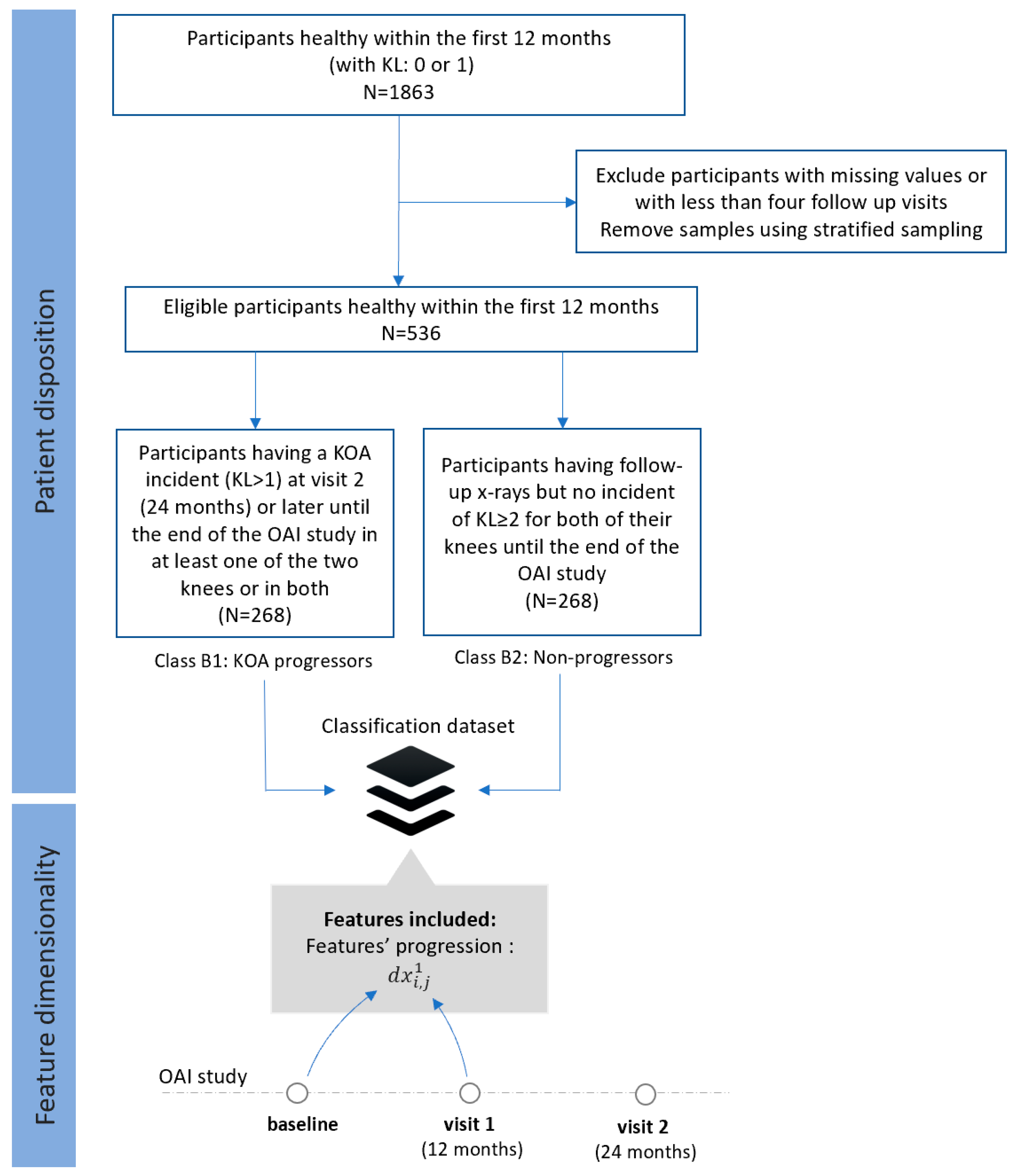
  • Dataset B (FS2): Progressors vs. non-progressors using progression data within the first 12 months
Input: Dataset B contains data that declares the features’ progression within the first 12 months. Specifically, the Equation (1) denotes the way that this progression was calculated.
d x i , j k =   x i , j k   x i , j 0       ,   j
where x i , j k and x i , j 0 are the j components (features) of sample x i measured at the visit k and the baseline (visit 0), respectively; d x i , j k is the calculated progression of x i , j within the time period between the k-th visit and the baseline and denotes the subset of features that co-exist in both visits (233 features for dataset B). As an example, let us consider the participant x 100 with a body mass index (P01BMI) of 20 at the baseline visit ( x 100 , 49 0 = 20, where j = 49 is the index of feature P01BMI). Let us also assume that the participant’s BMI at visit 1 has increased to 25 ( x 100 , 49 1 = 25). Thus, the BMI progression of the specific participant is calculated as d x 100 , 49 1 = 25 − 20 = 5. This calculation has been performed for all the 233 features of dataset B.
After data resampling, the following two classes of participants were created (Figure 2), as follows:
-
Class B1 (KOA progressors): This class comprises progression data d x i , j 1 of 268 participants who were healthy (KL 0 or 1) within the first 12 months (both at the baseline and the visit 1), but they had an incident of KL ≥ 2 at the second visit (24 months) or later (until the end of the OAI study).
-
Class B2 (non-progressors): This class involves progression data d x i , j 1 from 268 participants with KL 0 or 1 at the baseline, who had follow-up x-rays with no other incident of KL ≥ 2 in any of their knees until the end of the OAI study.
Output: Classification outputs 0 and 1 corresponding to assignments to classes B1 and B2, respectively.
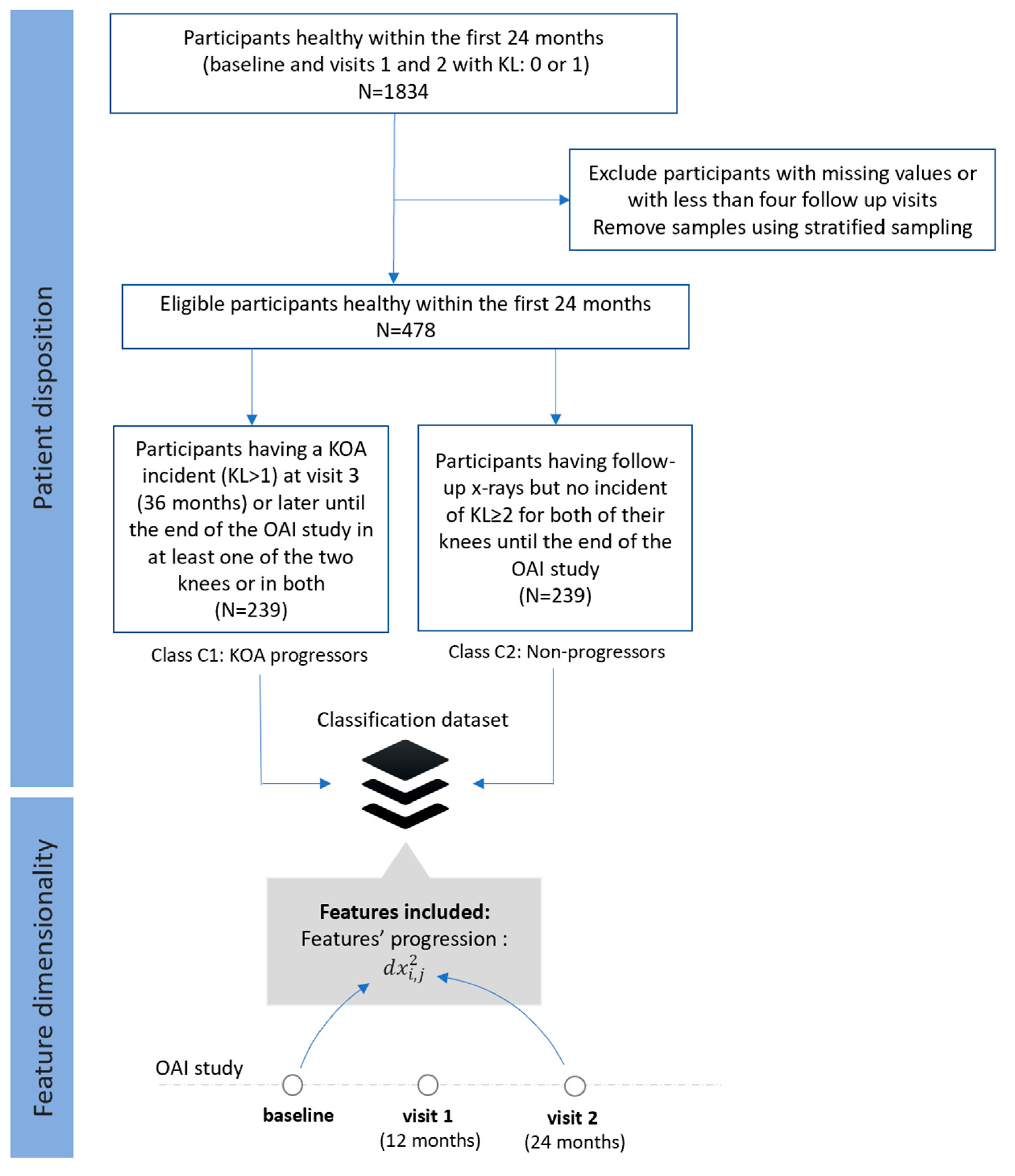
  • Dataset C (FS3): Progressors vs. non-progressors using progression data within the first 24 months
Input: Dataset C contains progression data d x i , j 2 within the first 24 months (until visit 2). The dataset contains 275 features that co-exist in visit 2 and the baseline, whereas the same methodology was used to calculate the features as given in Equation (1) using k = 2. The participants were divided into two equal categories (Figure 3), as follows:
-
Class C1 (KOA progressors): This class comprises of 239 participants who had KL 0 or 1 during the first 24 months, whereas a KOA incident (KL ≥ 2) observed at visit 3 (36 months) or later during the OAI course in at least one of the two knees or in both.
-
Class C2 (non-progressors): This class involves 239 participants with KL grade 0 or 1 at baseline, with follow-up X-rays and no further incidents (KL ≥ 2) for both of their knees.
Output: Classification outputs 0 and 1 corresponding to assignments to classes C1 and C2, respectively.
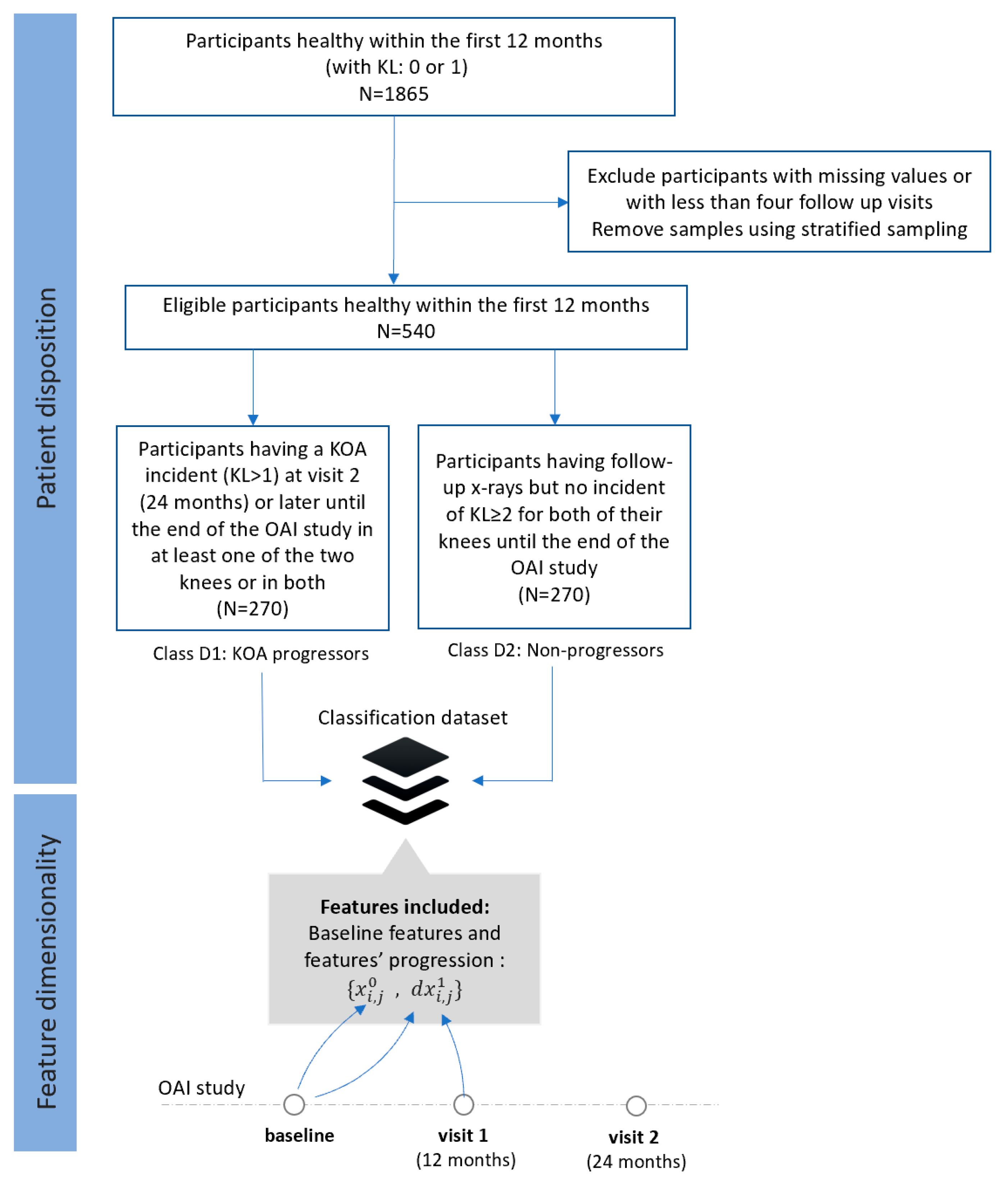
  • Dataset D (FS4): Progressors vs. non-progressors using data from the baseline visit along with progression data within the first 12 months
Input: Dataset D contains 957 features from both datasets A and B. Specifically, it consists of 957 features from the baseline ( x i , j 0   ,   j = 1 , , 724 ) along with progression data ( d x i , j 1   ,   j = 1 , ,   233 ) within the first 12 months. The list with the selected features from dataset D is given in Appendix A. After the application of data sampling, the participants were divided into two equal categories (Figure 4), as follows:
-
Class D1 (KOA progression): This class comprises 270 participants (KL 0 or 1) who were heathy during the first 12 months (with no incident at the baseline and the first visit) and then they had an incident (KL ≥ 2) recorded at their second visit (24 months) or later until the end of the OAI study.
-
Class D2 (non-KOA): This class involves 270 healthy participants with KL0 or 1 at baseline with no further incidents in both of their knees until the end of the OAI data collection.
Output: Classification outputs 0 and 1 corresponding to assignments to classes D1 and D2, respectively.
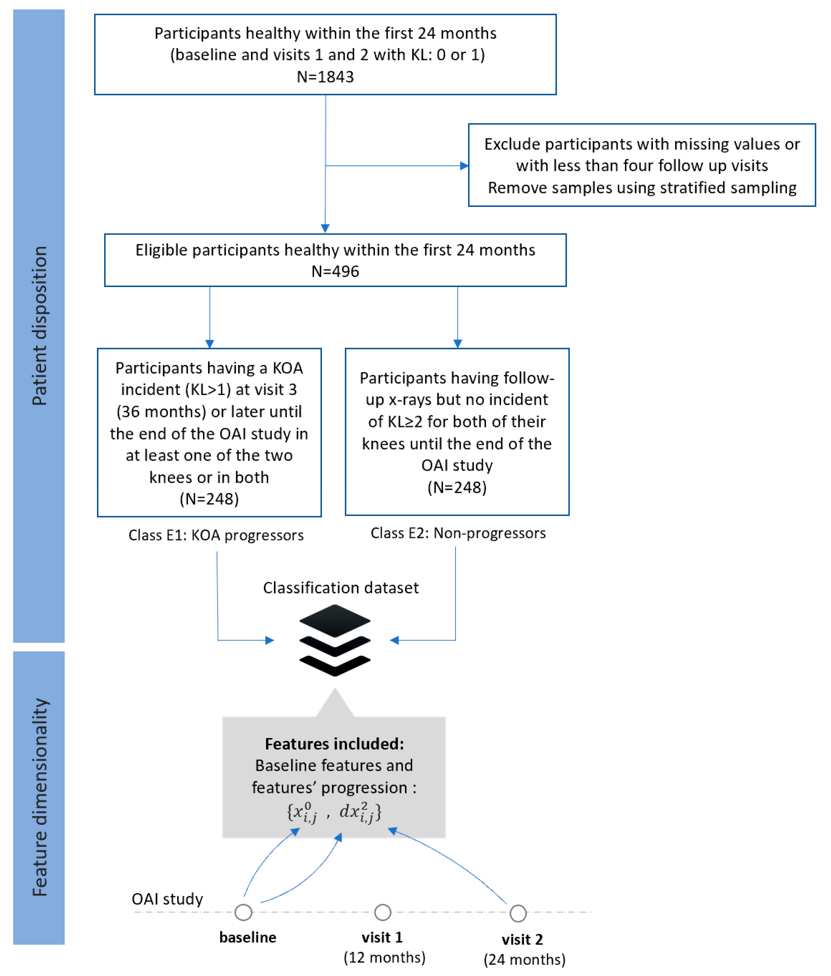
  • Dataset E (FS5): Progressors vs. non-progressors using data from the baseline visit along with progression data within the first 24 months
Input: Dataset E contains 999 features combining datasets A and C. This set of features consists of baseline data x i , j 0   ,   j = 1 , , 724 ) as well as progression data ( d x i , j 2 ,   j = 1 , , 275 ) within the first 24 months. Similarly, participants were divided into two equal categories (Figure 5), as follows:
-
Class E1 (KOA progression): This class comprises 248 participants who were healthy (KL 0 or 1) in the first 24 months, but they had a KOA incident (KL ≥ 2) at the third visit (36 months) or later until the end of the OAI study in at least one of the two knees or in both.
-
Class E2 (non-KOA): This class involves 248 healthy participants (KL0 or 1) with no further progression of KOA in both of their knees until the end of the OAI study.
Output: Classification outputs 0 and 1 corresponding to assignments to classes E1 and E2, respectively.

3. Methodology

The proposed in this paper ML methodology for KOA prediction includes four processing steps: (1) data pre-processing of the collected clinical data, (2) feature selection using the proposed approach, (3) learning process via the use of well-known ML models and (4) evaluation of the classification results. More details about the proposed methodology are presented in the following sections.

3.1. Pre-Processing

Data cleaning was initially performed by excluding the columns with more than 20% missing values compared to the total numbers of subjects. Subsequently, data imputation was performed to handle missing values. Specifically, mode imputation was implemented to replace missing values of the categorical or numerical variables by the mode (most frequent value) of the non-missing variables [18]. Standardization of a dataset is a common requirement for many ML estimators. In our paper, data was normalised to [0, 1] to build a common basis for the feature selection algorithms that follow [19]. Data resampling was employed to cope with the class imbalance problem. Specifically, the majority class was reduced in order to have the same number of samples as in the minority class.

3.2. Feature Selection (FS)

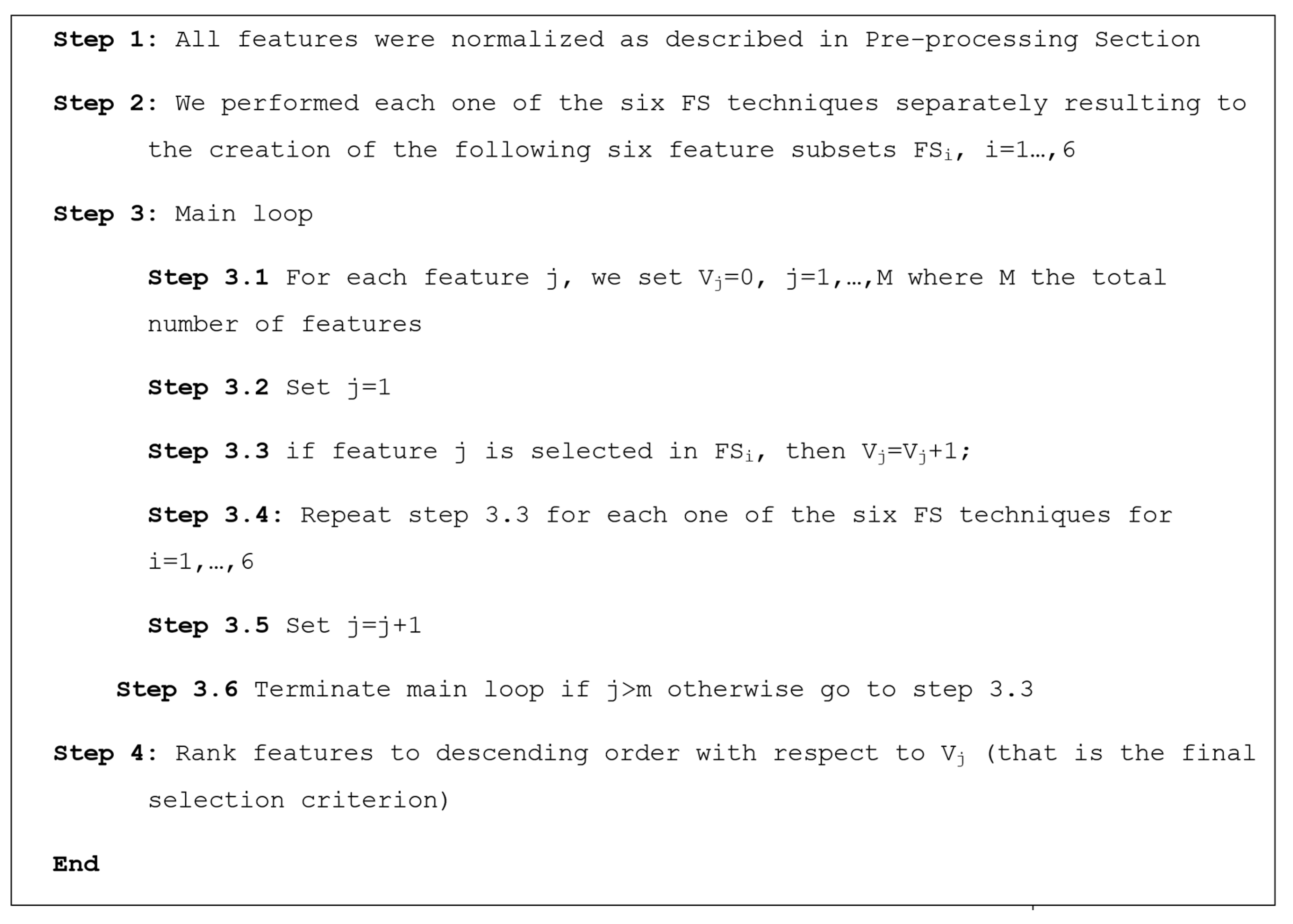
A robust feature selection methodology was employed that combined the outcomes of six FS techniques: two filter algorithms (Pearson correlation [20] and Chi-2 [21]), one wrapper (with logistic regression [22]) and three embedded ones (logistic regression L2 [23], random forest [24] and LightGBM [25]). Feature ranking was decided on the basis of a majority vote scheme. Specifically, we performed all six FS techniques separately, each one resulting into a selected FS. A feature receives a vote every time it has been selected by one of the FS algorithms. We finally ranked all features with respect to the votes received.
The proposed feature selection proceeds along the following steps as shown in Figure 6.

3.3. Learning Process

Various ML models were evaluated for their suitability in the task of KOA prediction. A brief description of these models is given below.
We tested logistic regression [26] which is likely the most commonly used algorithm for solving classification problems. Logistic regression models the probabilities for classification problems with two possible outcomes. It’s an extension of the linear regression model for classification problems. The interpretation of the weights in logistic regression differs from the interpretation of the weights in linear regression, since the outcome in logistic regression is a probability between 0 and 1. We also evaluated decision trees (DTs) [27] which are a non-parametric supervised learning method used for classification and regression. They are simple to understand and to interpret. DTs require little data preparation and perform well even if their assumptions are somewhat violated by the true model from which the data were generated.
K-Nearest Neighbor (KNN) [28] as well as non-linear support vector machines (SVM) algorithms [29], which can deal with the overfitting problems that appear in high-dimensional spaces. In the classification setting, the KNN algorithm essentially boils down to forming a majority vote between the K most similar instances to a given “unseen” observation. Similarity is defined according to a distance metric between two data points. A popular one is the Euclidean distance method. Furthermore, SVMs are a set of supervised learning methods used for classification, regression and outlier’s detection. They are effective in high dimensional spaces and still effective in cases where the number of dimensions is greater than the number of samples.
The ensemble technique Random Forest (RF) [30] was also evaluated using DT models as weak learners. RF classifier creates a set of decision trees from randomly selected subsets of training set. It then aggregates the votes from different decision trees to decide the final class of the test object. XGboost [31] and naive Bayes [32] algorithms were also considered. XGboost model is a sum of CART (tree) learners which try to minimize the log loss objective and the scores at leaves. These scores are actually the weights that have a meaning as a sum across all the trees of the model. Furthermore, they are always adjusted in order to minimize the loss. Moreover, naive Bayes methods are a set of supervised learning algorithms based on applying Bayes’ theorem with the “naive” assumption of conditional independence between every pair of features given the value of the class variable. Naive Bayes learners and classifiers can be extremely fast. The decoupling of the class conditional feature distributions means that each distribution can be independently estimated as a one-dimensional distribution.
Hyperparameter selection was implemented to optimize the performance of our models and to avoid overfitting and bias errors. Each model was optimized with respect to a number of preselected hyperparameters (Table 2). Specifically (i) ‘gamma’: [0, 0.4, 0.5, 0.6], ‘maximal depth’: [1, 2, 3, 4, 5, 6, 7, 8], ‘minimum child and weight’: [1, 3, 4, 5, 6, 8] were optimized for XGboost, (ii) ‘criterion’: [‘gini’, ’entropy’], ‘minimum samples leaf’: [1, 2, 3], ‘minimum samples split’: [3, 4, 5, 6, 7] and ‘number of estimators’: [10, 15, 20, 25, 30] for random forest, (iii) ‘maximal features’: [‘auto’, ‘sqrt’, ‘log2’], ‘minimum samples leafs’: [1, 2, 3, 4, 5, 6, 7, 8, 9, 10, 11] and ‘minimum number of decision splits’: [2, 3, 4, 5, 6, 7, 8, 9, 10, 11, 12, 13, 14, 15] for decision trees, (iv) ‘C’: [0.001, 0.01, 0.1, 1, 2, 3, 4, 5, 6, 7, 8, 9, 10] and ‘kernel’: [‘linear’,’sigmoid’,’rbf’,’poly’] for SVMs, (v) ‘k-parameter’: [5, 7, 9, 12, 14, 15, 16, 17] for KNN and (vi) ‘penalty’: [‘l1’, ‘l2’] and ‘C’: [100, 10, 1.0, 0.1, 0.01] for logistic regression.

3.4. Validation

A hold out 70–30% random data split was applied to generate the training and testing subsets, respectively. Learning of the ML was performed on the stratified version of the training sets and the final performance was estimated on the testing sets. We also evaluated the classifiers performance in terms of the confusion matrix as an additional evaluation criterion.
Confusion matrix is a way to evaluate the performance of a classifier. Specifically, a confusion matrix is a summary of prediction results on a classification problem (Table 3). To be created the confusion matrix, the number of correct (true) and incorrect (false) predictions are summarized with count values and broken down by each class.

4. Results

In this section, we present the most important risk factors as they have been selected by the proposed hybrid FS methodology. Moreover, the overall performance of the models is presented in relation to the number of selected features and then reference is made to the models with the highest accuracies. Results are initially given per dataset and an overall assessment is provided at the end. The efficacy of the proposed FS methodology is also compared with the performance of the six individual FS criteria.

4.1. Prediction Performance

The proposed ML methodology was applied on each of the five datasets. Specifically, the proposed FS was executed on the pre-processed versions of the datasets ranking the available features with respect to their relevance with the progression of OA. Then the proposed ML models were trained on feature subsets of increasing dimensionality (with a step of 5). These feature subsets were generated by sorting the features according to the selected ranking. This means that the proposed ML models were trained to classify KOA progressors and non-progressors based on the first (5, 10, 15, etc.) most informative features and the testing classification accuracies were finally calculated until the full feature set has been tested. The classification results on the five datasets are given below.
  • Dataset A
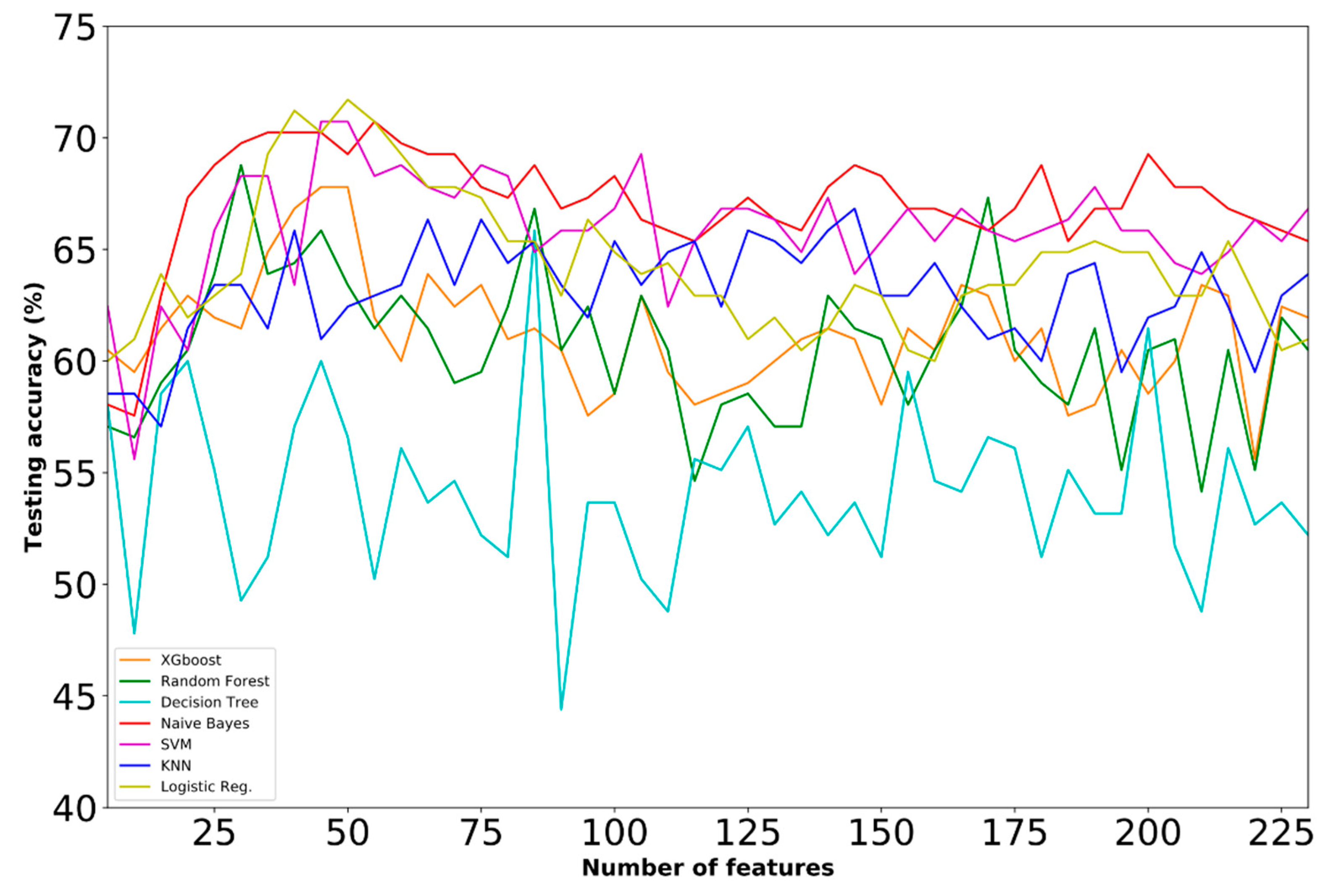
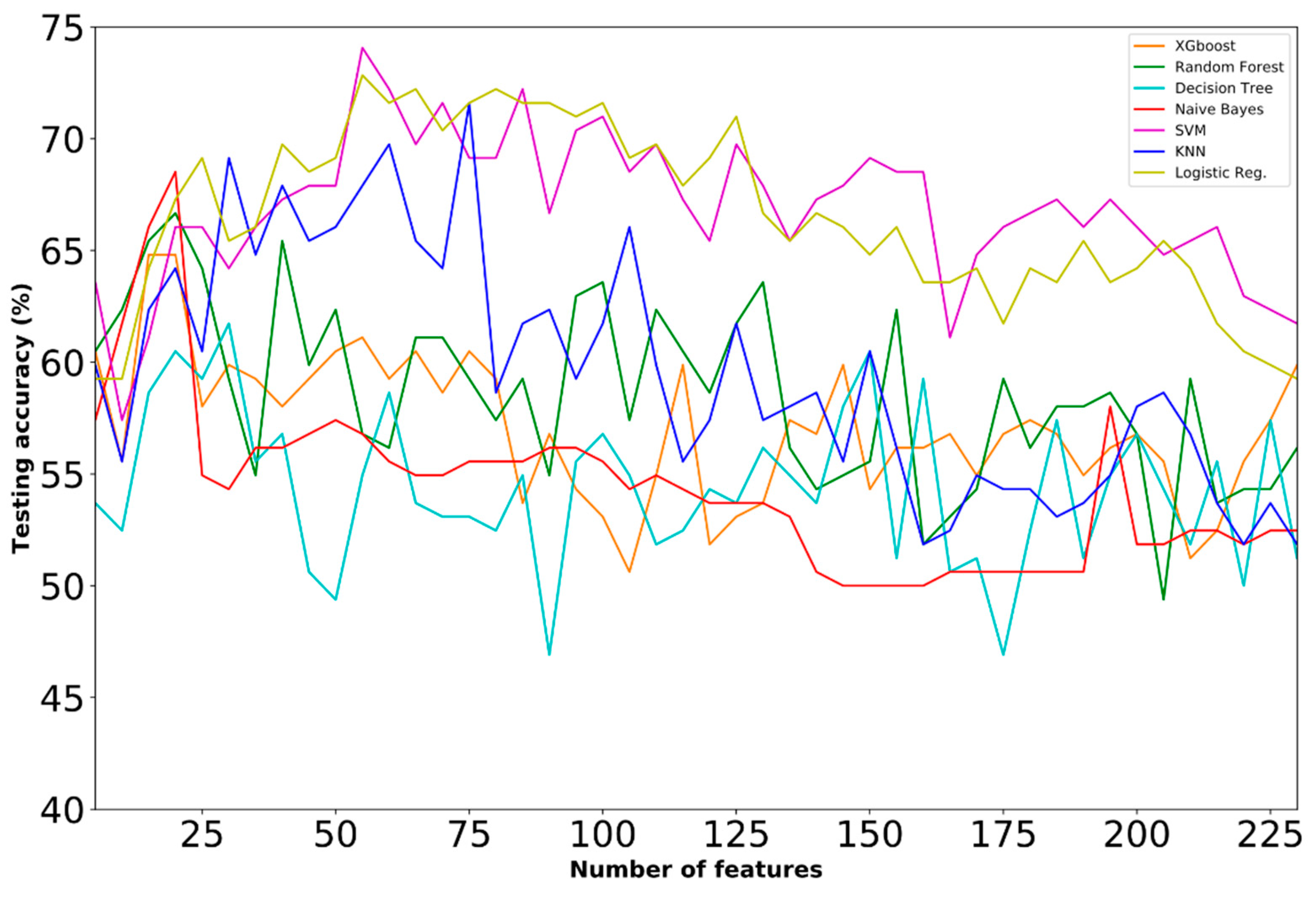
Figure 7 depicts the testing performance (%) of the competing ML models with respect to the number of selected features for dataset A. In particular, DTs failed in this task, recording low testing performances (in the range of 42.44–65.85%). In contrast, the other models had an upward trend in the first 20–60 features, followed by a steady testing performance in most of the cases. Specifically, the logistic regression model showed an upward trend with respect to selected features in the first 30–50 features, with a maximum of 71.71% at 50 features (which was the overall best performer). The inclusion of additional features led to a small reduction in the accuracies achieved.
Table 4 summarizes the results of logistic regression, XGboost, SVM, random forest, KNN, naive Bayes and DT on the two-class problem. A moderate number of features (in the range of 30–55) was finally selected by the majority of the ML models (in five out of the seven), whereas the overall maximum was achieved by LR on a group of fifty selected (50) risk factors. KNN and DTs selected more features (145 and 85, respectively) leading to low accuracies. The second highest accuracy was received for SVM and Naive Bayes (70.73% in both), whereas lower accuracies were obtained by NB, RF and XGboost.
  • Dataset B
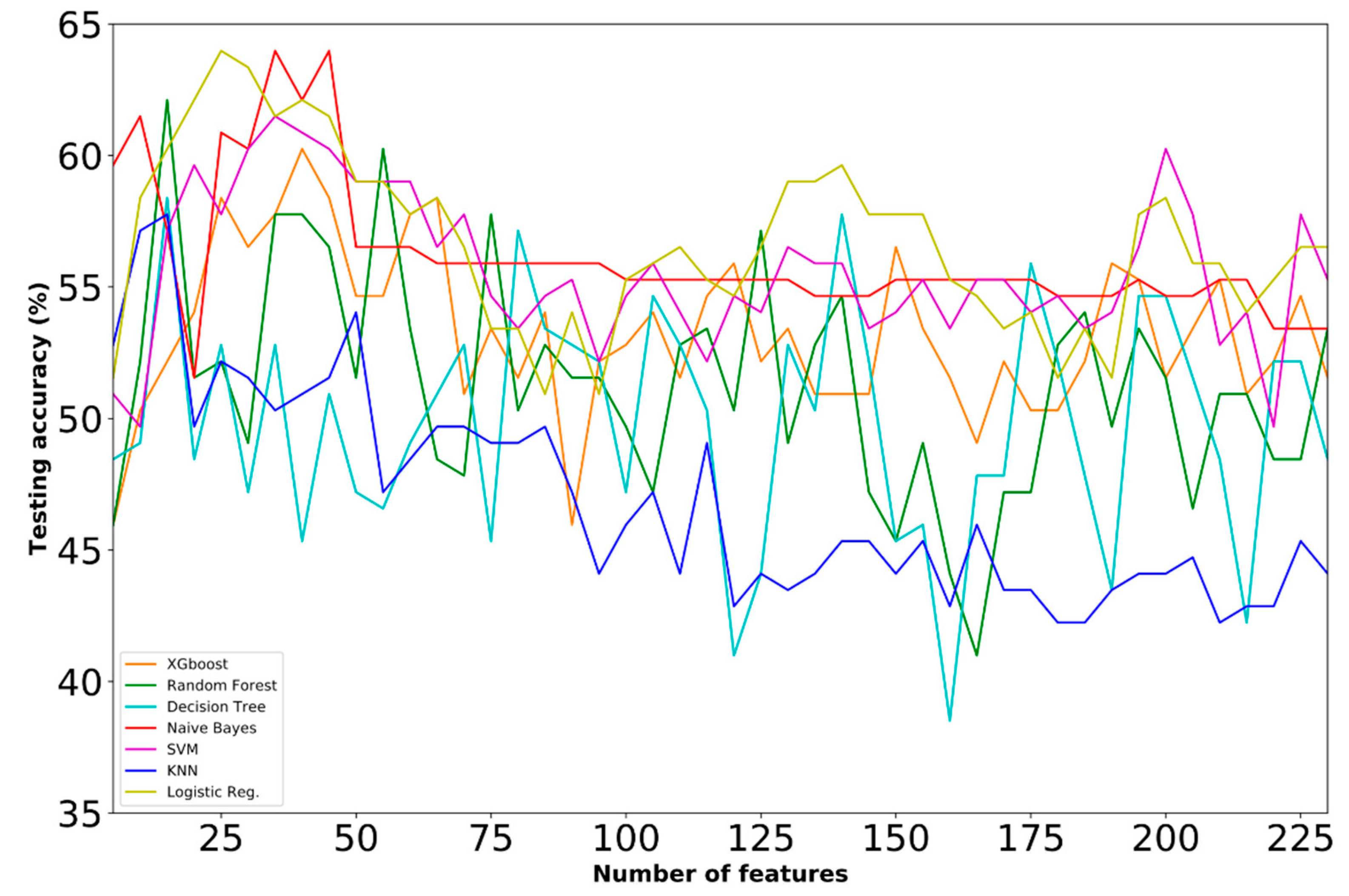
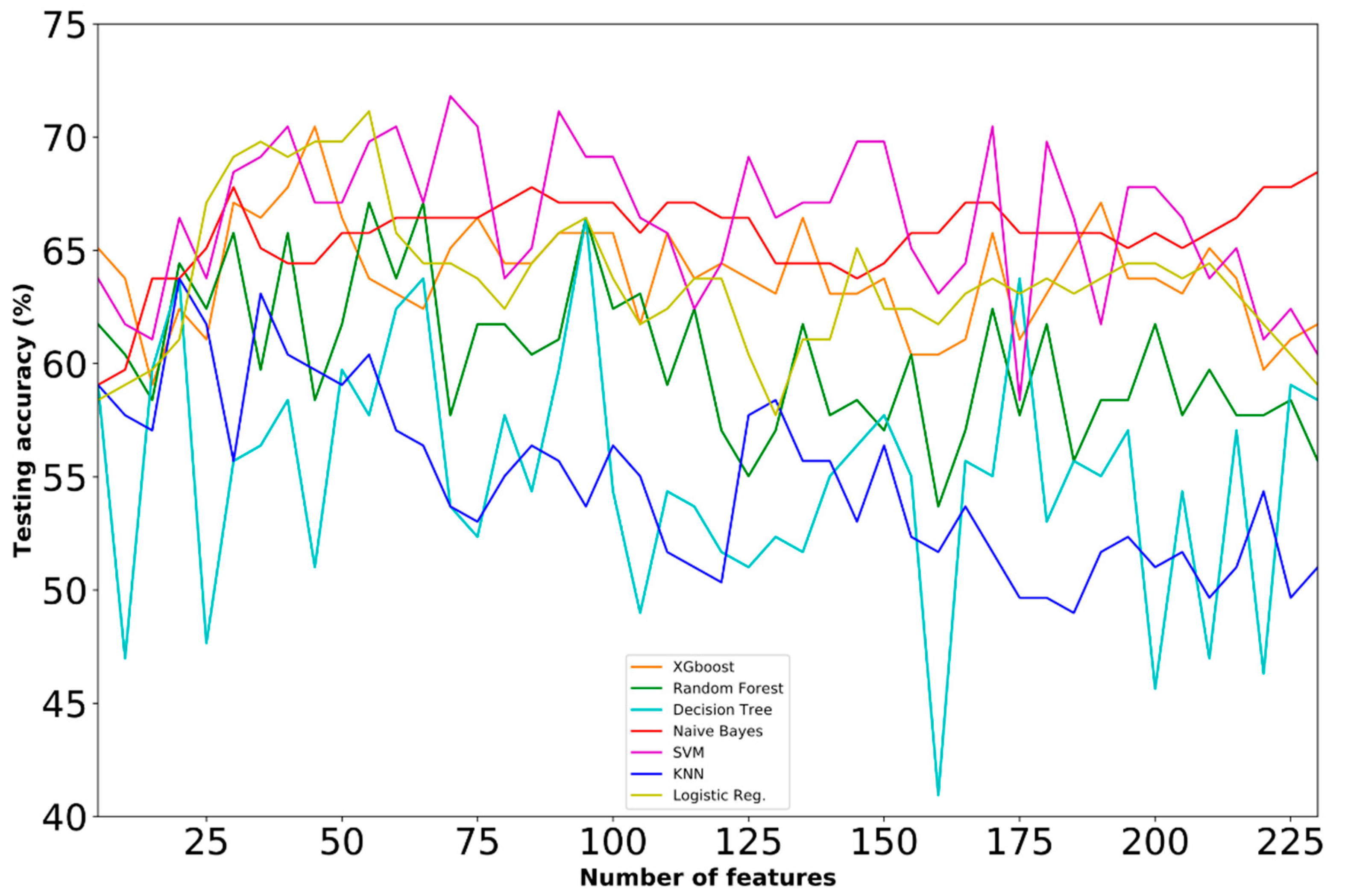
Figure 8 demonstrates the testing performance (%) of the competing ML models with respect to the number of selected features for dataset B. The following remarks could be extracted from Figure 8: (i) Considerably lower accuracies were achieved by all the competing ML models compared to the ones received in dataset A; (ii) LR and NB gave the maximum testing performance of approximately 64% at 25 features (which was the overall best performer in dataset B). The addition of more features did not increase the testing performance of the model but led to a reduction in the accuracies achieved. (iii) Low testing performances were accomplished by the rest of the ML models (in the range of 42.24–62.11%). The accuracies and confusion matrixes reported in Table 5 verify the aforementioned results. In all the competing models, the best accuracies were recorded using a relatively small number of selected risk factors (less or equal to 40).
  • Dataset C
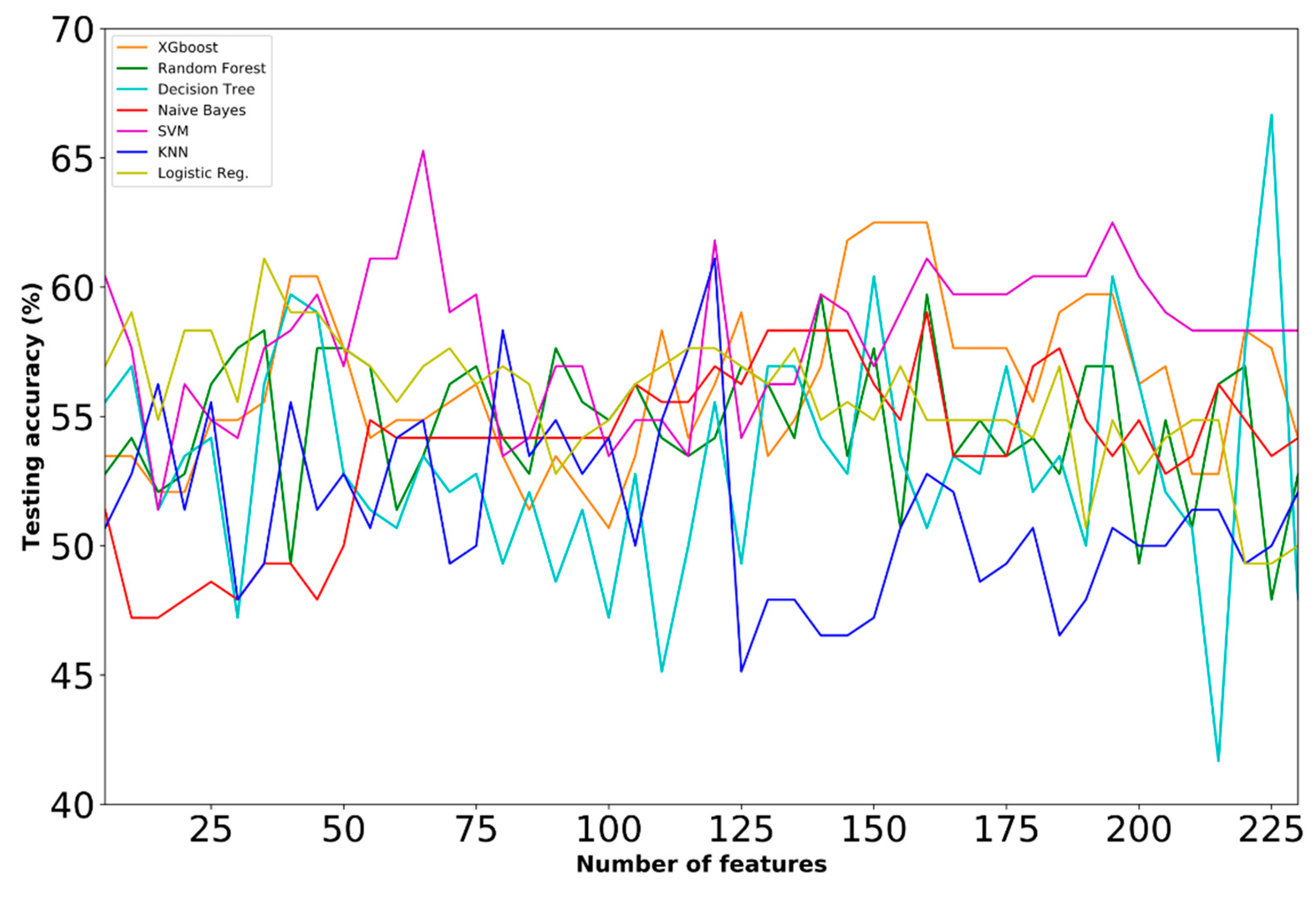
Less informative features with small generalization capacity are contained in dataset C, as reported in Figure 9 and Table 6. Unlike the previous two datasets, the best testing performance for dataset C was received at 225 features using DTs (66.67%). In general, unstable and low testing performances were observed for the majority of the employed ML models. The second highest accuracy was received for SVM (65.28%), whereas lower accuracies were obtained by the rest of the models. A significant number of features (more than 100) was also required in five out of the seven FS approaches highlighting the inability of dataset C features to provide useful information for the progression of KOA.
  • Dataset D
The combination of datasets A and B proved to be beneficial in the task of predicting KOA progression. Specifically, the following conclusions are drawn from the results reported in Figure 10 and Table 7: (i) The best performance (74.07%) was achieved by the SVM on the group of the fifty-five selected risk factors with linear kernel penalty and C = 0.1 (Dataset D). This performance was the overall best one achieved in all five datasets. (ii) The second highest accuracy was received for the logistic regression (72.84%), whereas lower accuracies were obtained by the rest of the models. (iii) SVM and LR followed a similar progression in the reported accuracies with respect to the number of selected features with an upward trend in the first 20–55 features, followed by a slight performance decrease as the number of features increases. (iv) KNN gave moderate results with a maximum testing performance of 71.6% at 75 selected features. (v) Low testing accuracies were obtained by RF, XGboost and DT in the range of 42.59–66.67%.
  • Dataset E
In dataset E, the SVM-based approach exhibited an upward trend with respect to selected features in the first 20–70 features, with a maximum of 71.81% at 70 features (which was the best in the category). The inclusion of additional features led to a small reduction in the accuracies achieved (Figure 11). Similarly to SVM, LR gave the second highest accuracy (71.14%) for less features (55). XGboost also gave a comparable performance (70.47%) in a subset of 45 selected features. Lower testing accuracies were received by the rest of ML models (Table 8).
Table 9 cites the best accuracies achieved in each of the five datasets. The combined effect of baseline features (dataset A) and progression data d x i , j 1 (dataset B) had a positive effect on the prediction capacity of the proposed methodology, as clearly shown in Table 7 where the testing accuracy in dataset D is increased by 2.36% compared to the result obtained in dataset A. A minor difference (0.1%) is observed on the accuracies reported for datasets A and E, demonstrating that d x i , j 2 progression data have a negligible effect on the predictive capacity of the proposed methodology and therefore could be omitted. The accuracies received in datasets B and C reveal that the baseline features are crucial for predicting KOA progression.

4.2. Selected Features

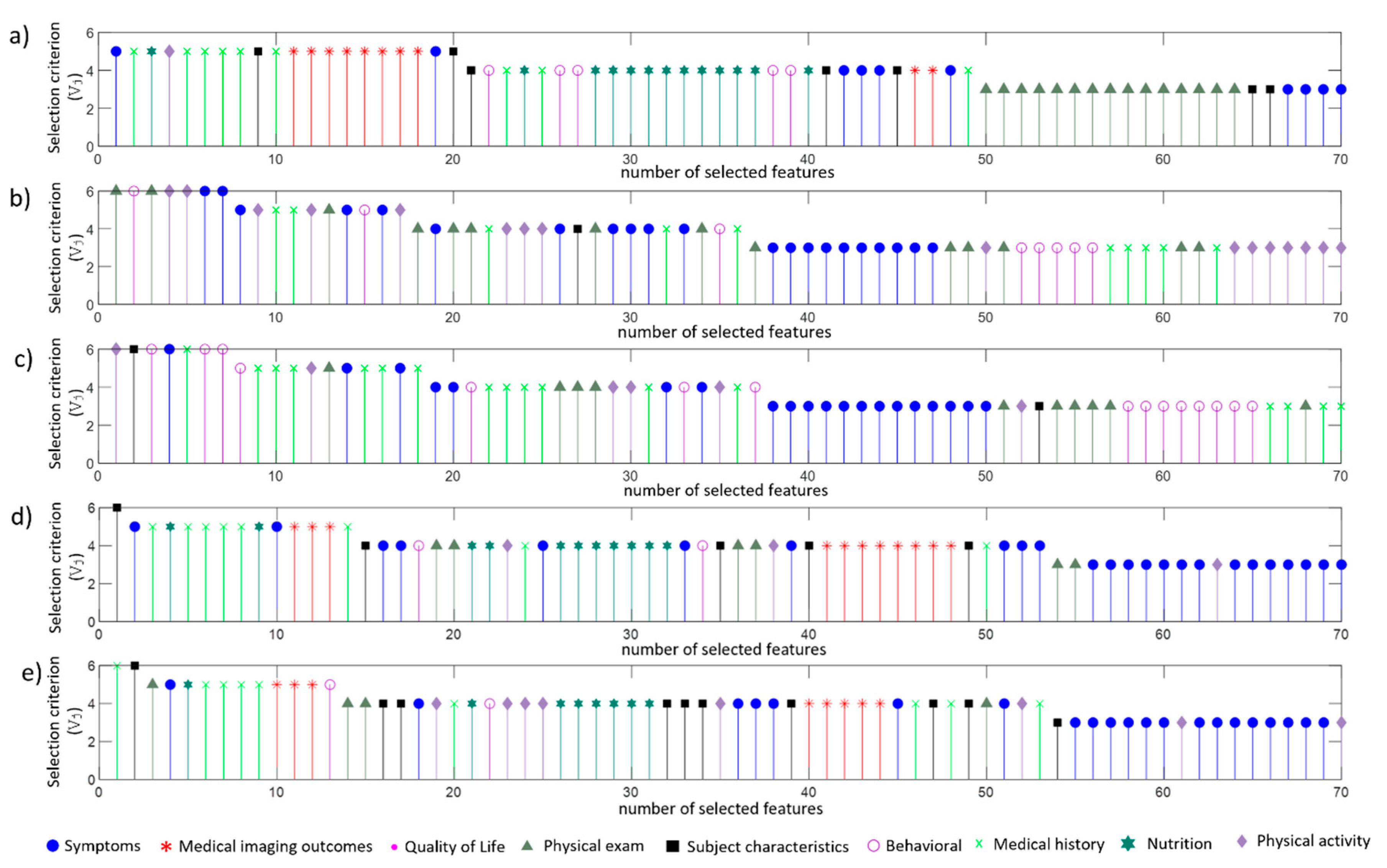
Figure 12 shows the first 70 features selected by the proposed FS approach for datasets A to E. Features are visualised with different colors and marks depending on the feature category they belong. The following conclusions could be drawn from the analysis of Figure 12: (i) Symptoms and medical imaging outcomes seem to be the most informative feature categories in dataset D in which the overall best performance was achieved. Specifically, eleven medical history outcomes and ten symptoms were selected in the first 55 features that gave the optimum prediction accuracy; (ii) nutrition and medical history characteristics were also proved to be contributing risk factors since approximately 20 out of the first selected 55 features were from these two feature categories (in dataset D). The full list of selected features for dataset D is provided in the appendix; (iii) similar results with respect to the selected features were extracted from the analyses in datasets A and E (in Figure 12a,e) that gave comparative prediction results (close to 72%); (iv) a different order in the selected features was observed in datasets B and C (as depicted in Figure 12b,c). The low accuracies recorded in these datasets (less than 67%) verify that the contained in these datasets features are less informative; (v) overall, it was concluded that a combination of heterogeneous features coming from almost all feature categories is needed to predict KL progression highlighting the necessity of adopting a multi-parametric approach that could handle the complexity of the available data.

4.3. Comparative Analysis

To evaluate the effectiveness of the proposed FS methodology, a comparison was performed in this section between the hybrid FS mechanism and the six well known FS techniques (the ones that are contained within the selection mechanism of the proposed methodology). The comparison was performed on dataset D that gave the overall best prediction performance. SVM was finally used to evaluate the prediction capacity of all the FS techniques considered here.
We performed and validated all six FS techniques separately, each one resulting into a different feature subset. SVM was finally trained on the resulted feature spaces of increasing dimensionality and the optimum feature subset was identified per case. As indicated in Table 10, the majority of the competing FS techniques provided lower testing performances compared to the proposed FS methodology. The wrapper technique based on LR was the only one that achieved an equal testing performance (%) with the proposed FS methodology. Specifically, the wrapper FS achieved its maximum accuracy at 70 features, while the proposed FS methodology achieved the same accuracy score using a smaller feature subset (55 features).

5. Discussion

This paper focuses on the development of a ML-empowered methodology for KL grades prediction in healthy participants. The prediction task has been coped as a two-class classification problem where the participants of the study were divided into two groups (KOA progressors and non-progressors). Various ML models were employed to perform the binary classification task (KOA progressors versus non-progressors) where accuracies up to 74.07% (Dataset D) were achieved. Within the secondary objectives of the paper were to identify informative risk factors from a big pool of available features that contribute more to the classification output (KOA prediction). Moreover, we explored different options with respect to the time period within which data should be considered in order to reliably predict KOA progression.
Three different options were investigated as far as the time period within which data should be considered in order to reliably predict KOA progression. To accomplish this, we worked with 5 different datasets. We first examined whether baseline data (dataset A) could solely contribute in predicting KOA progression. Going one step further, the features ‘progression within the first 12 months or 24 months was also considered as an alternative source of information (datasets B and C). The aforementioned analysis in Section 4 revealed that: (i) a 71.71% prediction performance can be achieved using features from the baseline, (ii) features’ progression cannot solely provide reliable KOA predictions and (iii) a combination of features is required to maximize the prediction capability of the proposed methodology. Specifically, the overall best accuracy (74.07%) was obtained by combining datasets A and B that contain features from the baseline visit along with their progression over the next 12 months. Considering a longer period of time (24 months) in the calculation of features’ progression resulted to lower prediction accuracies (71.81%).
The proposed FS methodology outperformed six well-known FS techniques achieving the best tradeoff between prediction accuracy and dimensionality reduction. From the pool of approximately 700 features of the OAI dataset, fifty-five were finally selected in this paper to predict KOA. As far as the nature of the selected features, it was concluded that symptoms, medical imaging outcomes, nutrition and medical history are the most important risk factors contributing considerably to the KOA prediction. However, it was also extracted that a combination of heterogeneous features coming from almost all feature categories is needed to effectively predict KL progression.
Seven ML algorithms were evaluated for their suitability in implementing the prediction task. Table 7 with the summary of all reporting result indicates that LR and SVM were proved to be the best performing models. The good performance of SVM could be attributed to the fact that SVM models are particularly well suited for classifying small or medium-sized complex datasets (both in terms of data size and dimensionality). LR was the second-best performer providing the highest prediction accuracy in datasets A and B and the second highest in datasets D and E. The fact that a generalized linear model such as LR accomplishes high performances indicates that the power of the proposed methodology lies on the effective and robust mechanism of selecting important risk factors and not so much on the complexity of the finally employed classifier. Identifying important features from the pool of heterogeneous health-related parameters (including anthropometrics, medical history, exams, medical outcomes, etc.) that are available nowadays is a key to increase our understanding of the KOA progression and therefore to provide robust prediction tools.
A few studies have recently addressed the problem of predicting KOA progression from different perspectives and employing different data sources. A weighted neighbor distance classifier was presented by Ashinsky et al. to classify isolated T2 maps for the progression to symptomatic OA with 75% accuracy [13]. Progression to clinical OA was defined by the development of symptoms as quantified by the WOMAC questionnaire 3 years after baseline evaluation. MRI images and PCA were employed by Du et al. to predict the progression of KOA using four ML techniques [33]. For KL grade prediction, the best performance was achieved by ANN with AUC = 0.761 and F-measure = 0.714. An MRI-based ML methodology has been also proposed by Marques et al. to prognose tibial cartilage loss via quantification of tibia trabecular bone where a odds ratio of 3.9 (95% confidence interval: 2.4–6.5) was achieved [15]. X-ray combined with pain scores have been utilized by Halilaj et al. to predict the progression of joint space narrowing (AUC = 0.86 using data from two visits spanning a year) and pain (AUC = 0.95 using data from a single visit) [6]. Similarly, another two studies (Tiulpin et al. [10] and Widera et al. [11]) made use of Xray images along with clinical data to predict KOA progression using either CNN or ML approaches achieving less accurate results. The current paper is the only one employing exclusively clinical non-imaging data and also contributes to the identification of important risk factors from a big pool of available features. The proposed methodology achieved comparable results with studies predicting KL grades progression demonstrating its uniqueness in facilitating prognosis of KOA progression with a less complicated ML methodology (without the need of big imaging data and image-based deep learning networks).
Among the limitations of the current study is the relatively large number of features (55) that were finally selected as possible predictors of KOA. The selected features come from almost all feature categories highlighting the necessity of adopting a rigorous data collection process in order to formulate the input feature vector that is needed for the ML training. Moreover, the ML models employed are opaque (black boxes) and therefore they are insufficient to provide explanations on the decisions (inability to explain how a certain output has been drawn). To overcome the aforementioned challenges, it is important for AI developers to build transparency into their algorithms and/or enhance the explainability of existing ML or DL networks.

6. Conclusions

This paper focuses on the development of a ML-based methodology capable of (i) predicting KOA progression (and specifically KL grades progression) and (ii) identifying important risk factors which contribute to the prediction of KOA. The proposed FS methodology combines well-known approaches including filter, wrapper and embedded techniques whereas feature ranking is decided on the basis of a majority vote scheme to avoid bias. Finally, a variety of ML models were built on the selected features to implement the KOA prediction task (treated as a two-class classification problem where a participant is classified to either the class of KOA progressors or to the non-progressors’ class). Apart from the selection of important risk factors, this paper also explores three different options with respect to the time period within which data should be considered in order to reliably predict KOA progression. The nature of the selected features was also discussed to increase our understanding of their effect on the KOA progression. After an extensive experimentation, a 74.07% classification accuracy was achieved by SVM on a group of fifty-five selected risk factors (in dataset D). Understanding the contribution of risk factors is a valuable tool for creating more powerful, reliable and non-invasive prognostic tools in the hands of physicians. For our future work, we are planning to also consider image-based biomarkers and areas with valuable information derived from biomechanical data that are expected to further improve the predictive capacity of the proposed methodology. ML explainability analysis will also be considered to capture the effect of the selected features on the models’ outcome.

Author Contributions

Data curation, C.K.; Funding acquisition, D.T.; Software, C.K.; Supervision, S.M., G.G. and D.T.; Validation, S.M., G.G. and D.T.; Writing–original draft, C.K.; Writing–review & editing, S.M., G.G. and D.T. All authors have read and agreed to the published version of the manuscript.

Funding

This research was funded by the European Community’s H2020 Programme, under grant agreement Nr. 777159 (OACTIVE).

Conflicts of Interest

The authors declare no conflict of interest.

Appendix A

Table A1. Selected features that led to the overall best Knee Osteoarthritis (KOA) prediction performance in our study.
FeatureDescription Category
1P02WTGAAbove weight cut-off for age/gender group (calc, used for study eligibility)Subject characteristics
2V00WPRKN2Right knee pain: stairs, last 7 daysSymptoms
3V00RXANALGRx Analgesic use indicator (calc)Medical history
4V00PCTSMALBlock Brief 2000: error flag, percent of foods marked as small portion (calc)Nutrition
5V00GLUCUsed glucosamine for joint pain or arthritis, past 6 monthsMedical history
6V00GLCFQCVGlucosamine frequency of use, past 6 months (calc)Medical history
7V00CHONUsed chondroitin sulfate for joint pain or arthritis, past 6 monthsMedical history
8V00CHNFQCVChondroitin sulfate frequency of use, past 6 months (calc)Medical history
9V00BAPCARBBlock Brief 2000: daily % of calories from carbohydrate, alcoholic beverages excluded from denominator (kcal) (calc)Nutrition
10P02KPNRCVRight knee pain, aching or stiffness: more than half the days of a month, past 12 months (calc, used for study eligibility)Symptoms
11P01XRKOABaseline radiographic knee OA status by person (calc)Medical imaging outcome
12P01SVLKOSTLeft knee baseline x-ray: evidence of knee osteophytes (calc)Medical imaging outcome
13P01OAGRDLLeft knee baseline x-ray: composite OA grade (calc)Medical imaging outcome
14P01GOUTCVDoctor said you had gout (calc)Medical history
15V00WTMAXKGMaximum adult weight, self-reported (kg) (calc)Subject characteristics
16V00WSRKN1Right knee stiffness: in morning, last 7 daysSymptoms
17V00WOMSTFRRight knee: WOMAC Stiffness Score (calc)Symptoms
18V00SF1In general, how is healthBehavioural
19V00RKMTTPNRight knee exam: medial tibiofemoral pain/tenderness present on examPhysical exam
20V00RFXCOMPIsometric strength: right knee flexion, able to complete (3) measurementsPhysical exam
21V00PCTFATBlock Brief 2000: daily percent of calories from fat (kcal) (calc)Nutrition
22V00PCTCARBBlock Brief 2000: daily percent of calories from carbohydrate (kcal) (calc)Nutrition
23V00PASEPhysical Activity Scale for the Elderly (PASE) score (calc)Physical activity
24V00LUNGCharlson Comorbidity: have emphysema, chronic bronchitis or chronicobstructive lung disease (also called COPD)Medical history
25V00KSXLKN1Left knee symptoms: swelling, last 7 daysSymptoms
26V00FFQSZ16Block Brief 2000: rice/dishes made with rice, how much each timeNutrition
27V00FFQSZ14Block Brief 2000: white potatoes not fried, how much each timeNutrition
28V00FFQSZ13Block Brief 2000: french fries/fried potatoes/hash browns, how much each timeNutrition
29V00FFQ69Block Brief 2000: regular soft drinks/bottled drinks like Snapple (not diet drinks), drink how often, past 12 monthsNutrition
30V00FFQ59Block Brief 2000: ice cream/frozen yogurt/ice cream bars, eat how often, past 12 monthsNutrition
31V00FFQ37Block Brief 2000: fried chicken, at home or in a restaurant, eat how often, past 12 monthsNutrition
32V00DTCAFFNBlock Brief 2000: daily nutrients from food, caffeine (mg) (calc)Nutrition
33V00DILKN11Left knee difficulty: socks off, last 7 daysSymptoms
34V00CESD13CES-D: how often talked less than usual, past weekBehavioural
35V00ABCIRCAbdominal circumference (cm) (calc)Subject characteristics
36TIMET120-m walk: trial 1 time to complete (sec.hundredths/sec)Physical exam
37STEPST120-m walk: trial 1 number of stepsPhysical exam
38PASE6Leisure activities: muscle strength/endurance, past 7 daysPhysical activity
39P02KPNLCVLeft knee pain, aching or stiffness: more than half the days of a month, past 12 months (calc, used for study eligibility)Symptoms
40P01WEIGHTAverage current scale weight (kg) (calc)Subject characteristics
41P01SVRKOSTRight knee baseline x-ray: evidence of knee osteophytes (calc)Medical imaging outcome
42P01SVRKJSLRight knee baseline x-ray: evidence of knee lateral joint space narrowing (calc)Medical imaging outcome
43P01RXRKOA2Right knee baseline x-ray: osteophytes and JSN (calc)Medical imaging outcome
44P01RXRKOARight knee baseline radiographic OA (definite osteophytes, calc, used in OAI definition of symptomatic knee OA)Medical imaging outcome
45P01RSXKOARight knee baseline symptomatic OA status (calc)Medical imaging outcome
46P01OAGRDRRight knee baseline x-ray: composite OA grade (calc)Medical imaging outcome
47P01LXRKOA2Left knee baseline x-ray: osteophytes and JSN (calc)Medical imaging outcome
48P01LXRKOALeft knee baseline radiographic OA (definite osteophytes, calc, used in OAI definition of symptomatic knee OA)Medical imaging outcome
49P01BMIBody mass index (calc)Subject characteristics
50P01ARTDRCVSeeing doctor/other professional for knee arthritis (calc)Medical history
51KSXRKN2Right knee symptoms: feel grinding, hear clicking or any other type of noise when knee moves, last 7 daysSymptoms
52KPRKN1Right knee pain: twisting/pivoting on knee, last 7 daysSymptoms
53DIRKN7Right knee difficulty: in car/out of car, last 7 daysSymptoms
54rkdefcvRight knee exam: alignment varus or valgus (calc)Physical exam
55lkdefcvLeft knee exam: alignment varus or valgus (calc)Physical exam

References

  1. Silverwood, V.; Blagojevic-Bucknall, M.; Jinks, C.; Jordan, J.; Protheroe, J.; Jordan, K. Current evidence on risk factors for knee osteoarthritis in older adults: A systematic review and meta-analysis. Osteoarthr. Cartil. 2015, 23, 507–515. [Google Scholar] [CrossRef] [PubMed] [Green Version]
  2. Ackerman, I.N.; Kemp, J.L.; Crossley, K.M.; Culvenor, A.G.; Hinman, R.S. Hip and Knee Osteoarthritis Affects Younger People, Too. J. Orthop. Sports Phys. Ther. 2017, 47, 67–79. [Google Scholar] [CrossRef] [PubMed]
  3. Lespasio, M.J.; Piuzzi, N.S.; Husni, M.E.; Muschler, G.F.; Guarino, A.; Mont, M.A. Knee osteoarthritis: A primer. Perm. J. 2017, 21. [Google Scholar] [CrossRef] [PubMed] [Green Version]
  4. Kokkotis, C.; Moustakidis, S.; Papageorgiou, E.; Giakas, G.; Tsaopoulos, D. Machine Learning in Knee Osteoarthritis: A Review. Osteoarthr. Cartil. Open 2020, 100069. [Google Scholar] [CrossRef]
  5. Lazzarini, N.; Runhaar, J.; Bay-Jensen, A.C.; Thudium, C.S.; Bierma-Zeinstra, S.M.A.; Henrotin, Y.; Bacardit, J. A machine learning approach for the identification of new biomarkers for knee osteoarthritis development in overweight and obese women. Osteoarthr. Cartil. 2017, 25, 2014–2021. [Google Scholar] [CrossRef] [Green Version]
  6. Halilaj, E.; Le, Y.; Hicks, J.L.; Hastie, T.J.; Delp, S.L. Modeling and predicting osteoarthritis progression: Data from the osteoarthritis initiative. Osteoarthr. Cartil. 2018, 26, 1643–1650. [Google Scholar] [CrossRef] [Green Version]
  7. Pedoia, V.; Haefeli, J.; Morioka, K.; Teng, H.L.; Nardo, L.; Souza, R.B.; Ferguson, A.R.; Majumdar, S. MRI and biomechanics multidimensional data analysis reveals R2 -R1rho as an early predictor of cartilage lesion progression in knee osteoarthritis. J. Magn. Reson. Imaging JMRI 2018, 47, 78–90. [Google Scholar] [CrossRef] [Green Version]
  8. Abedin, J.; Antony, J.; McGuinness, K.; Moran, K.; O’Connor, N.E.; Rebholz-Schuhmann, D.; Newell, J. Predicting knee osteoarthritis severity: Comparative modeling based on patient’s data and plain X-ray images. Sci. Rep. 2019, 9, 5761. [Google Scholar] [CrossRef]
  9. Nelson, A.; Fang, F.; Arbeeva, L.; Cleveland, R.; Schwartz, T.; Callahan, L.; Marron, J.; Loeser, R. A machine learning approach to knee osteoarthritis phenotyping: Data from the FNIH Biomarkers Consortium. Osteoarthr. Cartil. 2019, 27, 994–1001. [Google Scholar] [CrossRef]
  10. Tiulpin, A.; Klein, S.; Bierma-Zeinstra, S.M.; Thevenot, J.; Rahtu, E.; van Meurs, J.; Oei, E.H.; Saarakkala, S. Multimodal machine learning-based knee osteoarthritis progression prediction from plain radiographs and clinical data. Sci. Rep. 2019, 9, 20038. [Google Scholar] [CrossRef]
  11. Widera, P.; Welsing, P.M.; Ladel, C.; Loughlin, J.; Lafeber, F.P.; Dop, F.P.; Larkin, J.; Weinans, H.; Mobasheri, A.; Bacardit, J. Multi-classifier prediction of knee osteoarthritis progression from incomplete imbalanced longitudinal data. arXiv 2019, arXiv:1909.13408. [Google Scholar] [CrossRef] [PubMed]
  12. Alexos, A.; Moustakidis, S.; Kokkotis, C.; Tsaopoulos, D. Physical Activity as a Risk Factor in the Progression of Osteoarthritis: A Machine Learning Perspective. In International Conference on Learning and Intelligent Optimization; Springer: Cham, Switzerland, 2020; pp. 16–26. [Google Scholar]
  13. Ashinsky, B.G.; Bouhrara, M.; Coletta, C.E.; Lehallier, B.; Urish, K.L.; Lin, P.C.; Goldberg, I.G.; Spencer, R.G. Predicting early symptomatic osteoarthritis in the human knee using machine learning classification of magnetic resonance images from the osteoarthritis initiative. J. Orthop. Res. Official Publ. Orthop. Res. Soc. 2017, 35, 2243–2250. [Google Scholar] [CrossRef] [PubMed] [Green Version]
  14. Donoghue, C.; Rao, A.; Bull, A.M.J.; Rueckert, D. Manifold learning for automatically predicting articular cartilage morphology in the knee with data from the osteoarthritis initiative (OAI). Proc. Prog. Biomed. Opt. Imaging Proc. SPIE 2011, 7962, 79620E. [Google Scholar]
  15. Marques, J.; Genant, H.K.; Lillholm, M.; Dam, E.B. Diagnosis of osteoarthritis and prognosis of tibial cartilage loss by quantification of tibia trabecular bone from MRI. Magn. Reson. Med. 2013, 70, 568–575. [Google Scholar] [CrossRef] [PubMed]
  16. Yoo, T.K.; Kim, S.K.; Choi, S.B.; Kim, D.Y.; Kim, D.W. Interpretation of movement during stair ascent for predicting severity and prognosis of knee osteoarthritis in elderly women using support vector machine. In Proceedings of the 2013 35th Annual International Conference of the IEEE Engineering in Medicine and Biology Society (EMBC), Osaka, Japan, 3–7 July 2013; pp. 192–196. [Google Scholar] [CrossRef]
  17. Moustakidis, S.; Christodoulou, E.; Papageorgiou, E.; Kokkotis, C.; Papandrianos, N.; Tsaopoulos, D. Application of machine intelligence for osteoarthritis classification: A classical implementation and a quantum perspective. Quantum Mach. Intell. 2019. [Google Scholar] [CrossRef] [Green Version]
  18. Juszczak, P.; Tax, D.; Duin, R.P. Feature scaling in support vector data description. Proc. Asci 2002, 95–102. [Google Scholar]
  19. Dodge, Y.; Commenges, D. The Oxford Dictionary of Statistical Terms; Oxford University Press: Oxford, UK, 2006. [Google Scholar]
  20. Biesiada, J.; Duch, W. Feature selection for high-dimensional data—A Pearson redundancy based filter. In Computer Recognition Systems 2; Springer: Berlin/Heidelberg, Germany, 2007; pp. 242–249. [Google Scholar]
  21. Thaseen, I.S.; Kumar, C.A. Intrusion detection model using fusion of chi-square feature selection and multi class SVM. J. King Saud Univ. Comput. Inf. Sci. 2017, 29, 462–472. [Google Scholar]
  22. Xiong, M.; Fang, X.; Zhao, J. Biomarker identification by feature wrappers. Genome Res. 2001, 11, 1878–1887. [Google Scholar] [CrossRef] [Green Version]
  23. Nie, F.; Huang, H.; Cai, X.; Ding, C.H. Efficient and robust feature selection via joint ℓ2, 1-norms minimization. In Proceedings of the Advances in neural information processing systems, Vancouver, BC, Canada, 6–9 December 2010; pp. 1813–1821. [Google Scholar]
  24. Zhou, Q.; Zhou, H.; Li, T. Cost-sensitive feature selection using random forest: Selecting low-cost subsets of informative features. Knowl. Based Syst. 2016, 95, 1–11. [Google Scholar] [CrossRef]
  25. Al Daoud, E. Comparison between XGBoost, LightGBM and CatBoost Using a Home Credit Dataset. Int. J. Comput. Inf. Eng. 2019, 13, 6–10. [Google Scholar]
  26. Rockel, J.S.; Zhang, W.; Shestopaloff, K.; Likhodii, S.; Sun, G.; Furey, A.; Randell, E.; Sundararajan, K.; Gandhi, R.; Zhai, G. A classification modeling approach for determining metabolite signatures in osteoarthritis. PLoS ONE 2018, 13, e0199618. [Google Scholar] [CrossRef] [PubMed]
  27. Kobayashi, T.; Kannari, T.; Horiuchi, H.; Matsui, N.; Ito, T.; Nojin, K.; Kakuse, K.; Okawa, M.; Yamanaka, M. Predictors affecting balance performances in patients with knee osteoarthritis using decision tree analysis. Osteoarthr. Cartil. 2019, 27, S243. [Google Scholar] [CrossRef] [Green Version]
  28. Peterson, L.E. K-nearest neighbor. Scholarpedia 2009, 4, 1883. [Google Scholar] [CrossRef]
  29. Gornale, S.S.; Patravali, P.U.; Marathe, K.S.; Hiremath, P.S. Determination of Osteoarthritis Using Histogram of Oriented Gradients and Multiclass SVM. Int. J. Image Graph. Signal Process. 2017, 9. [Google Scholar] [CrossRef] [Green Version]
  30. Kotti, M.; Duffell, L.D.; Faisal, A.A.; McGregor, A.H. Detecting knee osteoarthritis and its discriminating parameters using random forests. Med. Eng. Phys. 2017, 43, 19–29. [Google Scholar] [CrossRef] [PubMed]
  31. Torlay, L.; Perrone-Bertolotti, M.; Thomas, E.; Baciu, M. Machine learning–XGBoost analysis of language networks to classify patients with epilepsy. Brain Inform. 2017, 4, 159–169. [Google Scholar] [CrossRef] [PubMed]
  32. Du, Y.; Shan, J.; Zhang, M. Knee osteoarthritis prediction on MR images using cartilage damage index and machine learning methods. In Proceedings of the Proceedings—2017 IEEE International Conference on Bioinformatics and Biomedicine, BIBM, Kansas City, MO, USA, 13–16 November 2017; pp. 671–677. [Google Scholar]
  33. Du, Y.; Almajalid, R.; Shan, J.; Zhang, M. A Novel Method to Predict Knee Osteoarthritis Progression on MRI Using Machine Learning Methods. IEEE Trans. Nanobiosci. 2018. [Google Scholar] [CrossRef]
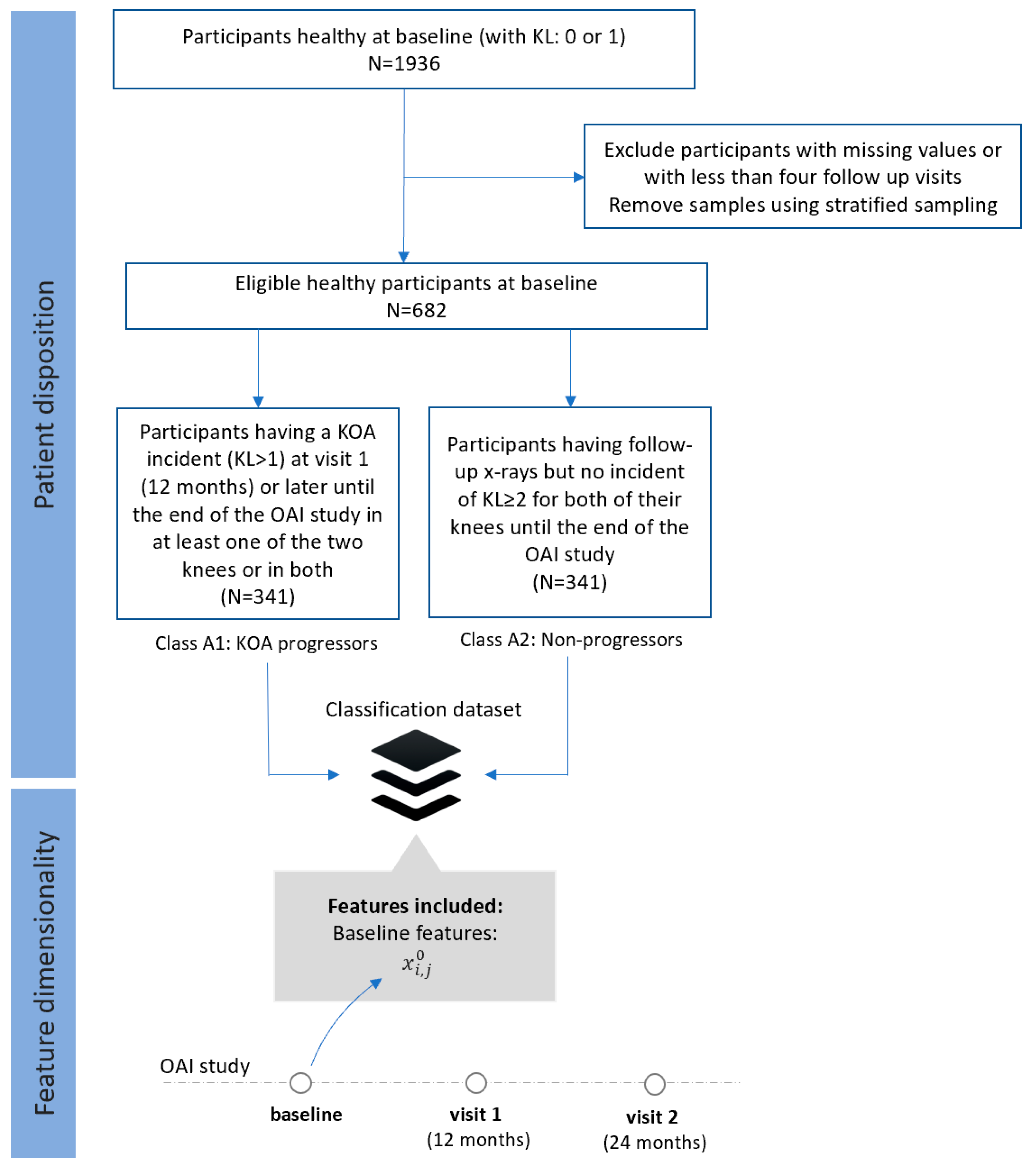
Figure 1. Flow chart of study design for dataset A.
Applsci 10 06797 g001
Figure 2. Flow chart of study design for dataset B.
Applsci 10 06797 g002
Figure 3. Flow chart of study design for dataset C.
Applsci 10 06797 g003
Figure 4. Flow chart of study design for dataset D.
Applsci 10 06797 g004
Figure 5. Flow chart of study design for dataset E.
Applsci 10 06797 g005
Figure 6. Pseudocode for the implementation of the proposed feature selection (FS).
Applsci 10 06797 g006
Figure 7. Learning curves with testing accuracy scores on dataset A for different machine learning (ML) models trained on feature subsets of increasing dimensionality.
Applsci 10 06797 g007
Figure 8. Learning curves with testing accuracy scores on dataset B for different ML models trained on feature subsets of increasing dimensionality.
Applsci 10 06797 g008
Figure 9. Learning curves with testing accuracy scores on dataset C for different ML models trained on feature subsets of increasing dimensionality.
Applsci 10 06797 g009
Figure 10. Learning curves with testing accuracy scores on dataset D for different ML models trained on feature subsets of increasing dimensionality.
Applsci 10 06797 g010
Figure 11. Learning curves with testing accuracy scores on dataset E for different ML models trained on feature subsets of increasing dimensionality.
Applsci 10 06797 g011
Figure 12. Features selected in datasets A to E in (ae), respectively. Axis y (selection criterion) denotes how many times a feature has been selected (6 declares that a specific feature has been selected by all six FS techniques and so on). Features have been ranked based on the selection criterion Vj and are visualised with different colors each one representing a specific feature category.
Applsci 10 06797 g012
Table 1. Main categories of the feature subsets considered in this paper.
Timeline of Visit
CategoryDescriptionBaseline12 Months24 Months
Subject characteristicsAnthropometric parameters including height, weight, BMI, abdominal circumference, etc.
BehaviouralParticipants’ social behaviour and quality level of daily routine
Medical historyQuestionnaire data regarding a Participant’s arthritis-related and general health histories and medications--
Medical imaging outcomeMedical imaging outcomes (e.g., osteophytes and joint space narrowing)--
NutritionBlock Food
Frequency questionnaire
--
Physical activityQuestionnaire results regarding leisure activities, etc.
Physical examPhysical measurements of participants, including isometric strength, knee and hand exams, walking tests and other performance measures
SymptomsArthritis symptoms and general arthritis or health-related function and disability
Table 2. Hyperparameters description.
ML ModelsHyperparametersDescription
XGboostGammaMinimum loss reduction required to make a further partition on a leaf node of the tree.
Maximal depthMaximum depth of a tree. Increasing this value will make the model more complex and more likely to overfit.
Minimum child and WeightMinimum sum of instance weight (hessian) needed in a child. If the tree partition step results in a leaf node with the sum of instance weight less than min_child_weight, then the building process will give up further partitioning.
Random ForestCriterionThe function to measure the quality of a split.
Minimum samples leafThe minimum number of samples required to be at a leaf node.
Number of estimatorsThe number of trees in the forest.
Decision TreesMaximal featuresThe number of features to consider when looking for the best split.
Minimum samples splitThe minimum number of samples required to split an internal node
Minimum number of leafsThe minimum number of samples required to be at a leaf node.
SVMsCRegularization parameter. The strength of the regularization is inversely proportional to C.
KernelSpecifies the kernel type to be used in the algorithm.
KNNk-parameterNumber of neighbors to use by default for k neighbors queries.
Logistic RegressionPenaltyUsed to specify the norm used in the penalization.
CInverse of regularization strength; must be a positive float.
Table 3. Confusion matrix.
Actual Classes
PositiveNegative
Predicted classesPositiveTrue PositiveFalse Positive
NegativeFalse NegativeTrue Negative
Table 4. Best testing accuracies achieved for ML model along with the confusion matrix, the optimum number of features and the hyperparameters of the ML models employed. A1 and A2 denote classes 1 and 2 of dataset A, respectively.
ModelsAccuracy (%)Confusion MatrixFeaturesParameters
Logistic Regression71.71 A1A250Penalty: l1, C: 1.0
A17328
A23074
Naive Bayes70.73 A1A255GaussianNB
A17229
A23173
SVM70.73 A1A245C = 2, kernel = sigmoid
A17526
A23470
KNN66.83 A1A2145leaf_size: 1, n_neighbors: 12, weights: distance
A17823
A24559
Decision Tree65.85 A1A285max_features: log2, min_samples_leaf: 4, min_samples_split: 11
A16833
A23767
Random Forest68.78 A1A230criterion: gini, min_samples_leaf: 3, min_samples_split: 7, n_estimators: 15
A17130
A23470
XGboost67.8 A1A245gamma: 0, max_depth: 1, min_child_weight: 4
A16932
A23470
Table 5. Best testing accuracies achieved for each ML model along with the confusion matrix, the optimum number of features and the hyperparameters of the ML models employed. B1 and B2 denote classes 1 and 2 of dataset B, respectively.
ModelsAccuracy (%)Confusion MatrixFeaturesParameters
Logistic Regression63.98 B1B225Penalty: l1, C: 1.0
B14822
B23655
Naive Bayes63.98 B1B235GaussianNB
B15020
B23853
SVM61.49 B1B235C: 6, kernel: linear
B14624
B23853
KNN57.76 B1B215leaf_size: 1, n_neighbors: 16, weights: uniform
B1637
B26130
Decision Tree58.39 B1B215max_features: auto, min_samples_leaf: 1, min_samples_split: 6
B14129
B23853
Random Forest62.11 B1B215criterion: gini, min_samples_leaf: 2, min_samples_split: 7, n_estimators: 30
B14822
B23952
XGboost60.25 B1B240gamma: 0.4, max_depth: 7, min_child_weight: 5
B14426
B23853
Table 6. Best testing accuracies achieved for each ML model along with the confusion matrix, the optimum number of features and the hyperparameters of the ML models employed. C1 and C2 denote classes 1 and 2 of dataset C, respectively.
ModelsAccuracy (%)Confusion MatrixFeaturesParameters
Logistic Regression61.11 C1C235Penalty: l1, C: 1.0
C14915
C24139
Naive Bayes59.03 C1C2160GaussianNB
C12341
C21862
SVM65.28 C1C265C: 5, kernel: rbf
C14816
C23446
KNN61.11 C1C2120leaf_size: 1, n_neighbors: 5, weights: uniform
C1559
C24733
Decision Tree66.67 C1C2225max_features: auto, min_samples_leaf: 2, min_samples_split: 8
C14420
C22852
Random Forest59.72 C1C2140criterion: gini, min_samples_leaf’: 1, min_samples_split: 5, n_estimators: 25
C13727
C23149
XGboost62.5 C1C2150n_estimators = 100, max_depth = 8, learning_rate = 0.1, subsample = 0.5
C14420
C23446
Table 7. Best testing accuracies achieved for each ML model along with the confusion matrix, the optimum number of features and the hyperparameters of the ML models employed. D1 and D2 denote classes 1 and 2 of dataset D, respectively.
ModelsAccuracy (%)Confusion MatrixFeaturesParameters
Logistic Regression72.84 D1D255Penalty: l1, C: 1.0
D15427
D21764
Naive Bayes68.52 D1D220GaussianNB
D14437
D21467
SVM74.07 D1D255C: 0.1, kernel: linear
D15625
D21764
KNN71.6 D1D275algorithm: auto, leaf_size: 1, n_neighbors: 17, weights: uniform
D15526
D22061
Decision Tree61.73 D1D230max_features: auto, min_samples_leaf: 3, min_samples_split: 10
D15625
C23744
Random Forest66.67 D1D220criterion: gini, min_samples_leaf: 3, min_samples_split: 3, n_estimators: 25
D14734
D22061
XGboost64.81 D1D215gamma: 0.6, max_depth: 1, min_child_weight: 8
D15130
D22754
Table 8. Best testing accuracies achieved for each ML model along with the confusion matrix, the optimum number of features and the hyperparameters of the ML models employed. E1 and E2 denote classes 1 and 2 of dataset E, respectively.
ModelsAccuracy (%)Confusion MatrixFeaturesParameters
Logistic Regression71.14 E1E255Penalty: l1, C: 1.0
E15017
E22656
Naive Bayes68.46 E1E2230GaussianNB
E14819
E22854
SVM71.81 E1E270C: 1, kernel: sigmoid
E15017
E22557
KNN63.76 E1E220algorithm: auto, leaf_size: 1, n_neighbors: 16, weights: uniform
E14819
E23547
Decision Tree66.44 E1E295max_features: auto, min_samples_leaf: 2, min_samples_split: 12
E14522
E22854
Random Forest67.11 E1E255criterion: gini, min_samples_leaf: 1, min_samples_split: 3, n_estimators: 30
E14225
E22458
Xgboost70.47 E1E245gamma: 0.6, max_depth: 2, min_child_weight: 1
E14324
E22062
Table 9. Summary of all reported results.
DatasetData Used in the TrainingBest Testing Performance (%) AchievedBest ModelNum. of Selected Features
BaselineM12 Progress Wrt BeselineM24 Progress Wrt Baseline
A 71.71Logistic Regression50
B 63.98Logistic Regression25
C 66.67Decision Tree225
D 74.07SVM55
E 71.81SVM70
Table 10. Testing performance (%) of the competing FS techniques with respect to the number of selected features for dataset D.
FS Criteria
Filter AlgorithmsWrapper AlgorithmsEmbeddedProposed FS Criterion
FeaturesChi-2PearsonLogistic RegressionLogistic Regression (L2)Random ForestLightGBM
558.0262.3562.9654.3245.6856.1763.58
1063.5863.5859.8851.2348.7750.0057.41
1561.1158.0251.8550.6250.6253.7061.11
2053.0961.1157.4148.7750.6250.0066.05
2560.4965.4360.4951.8556.7953.7066.05
3064.8170.3770.3760.4958.0251.2364.2
3566.6765.4362.9656.7958.0253.7066.05
4059.2666.6765.4360.4960.4954.3267.28
4564.8167.9069.7554.3258.0246.3067.9
5063.5867.2868.5255.5660.4948.7767.9
5564.8169.7564.8153.0959.8853.0974.07
6069.7567.2865.4355.5659.8855.5672.22
6561.7364.8170.9960.4958.6454.9469.75
7068.5266.6774.0756.1756.1754.3271.6
7568.5264.8172.2254.3251.8559.2669.14
8066.0566.6769.1458.0258.0259.8869.14
8566.0566.6772.8453.7059.2657.4172.22
9067.9056.7973.4658.6462.9653.0966.67
9566.6756.7969.1459.8861.1155.5670.37
10062.9659.8872.2261.7356.7955.5670.99