A Fast Ray-tracing Method for Locating Mining-Induced Seismicity by Considering Underground Voids


Abstract
Featured Application
Abstract
1. Introduction
2. Methodology
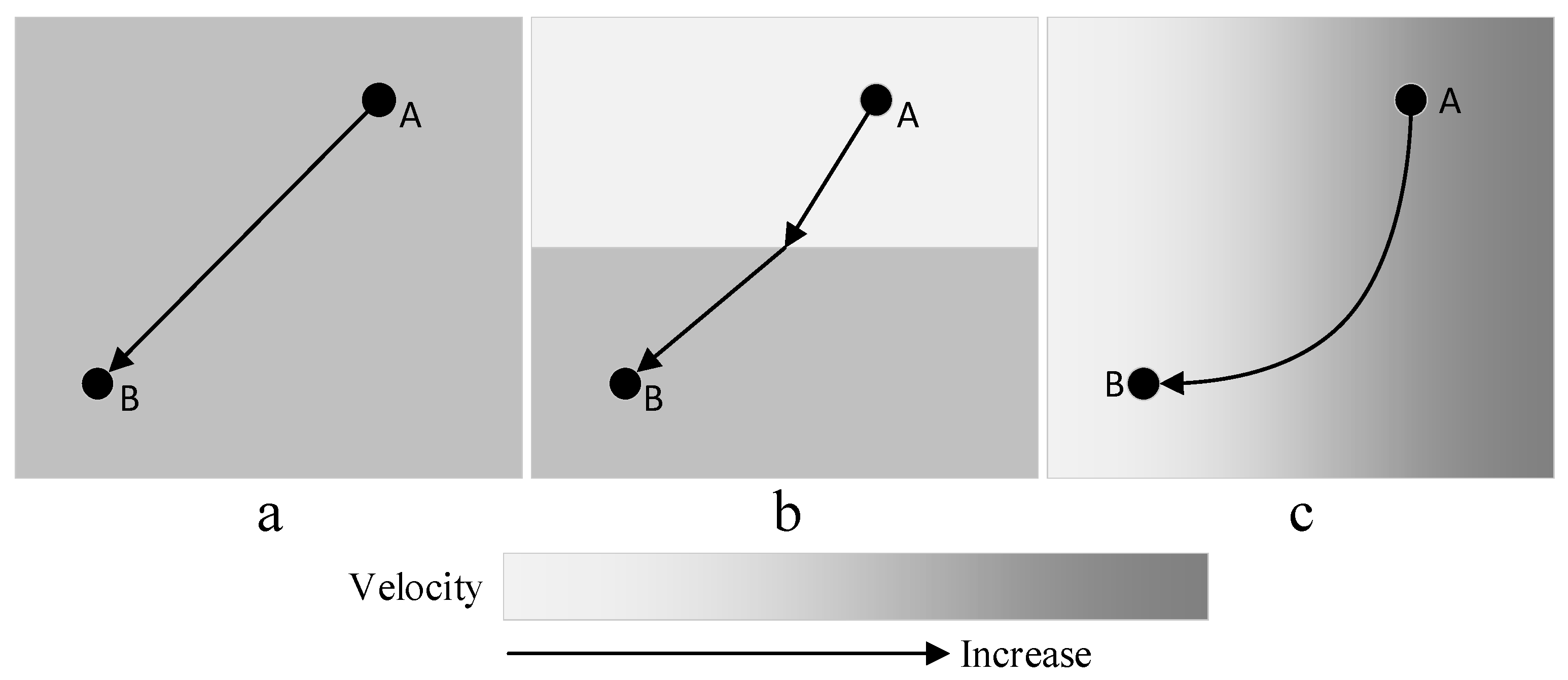
2.1. Fermat Principle
2.2. A Fast Ray-tracing Method
2.2.1. Modeling
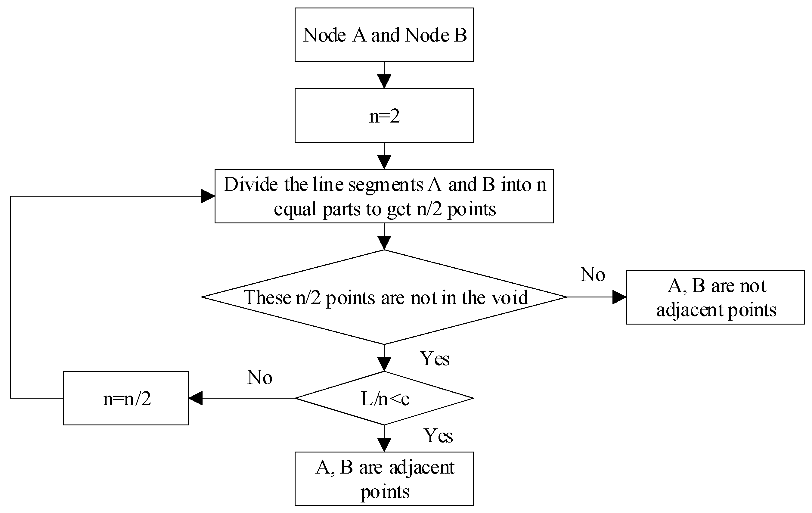
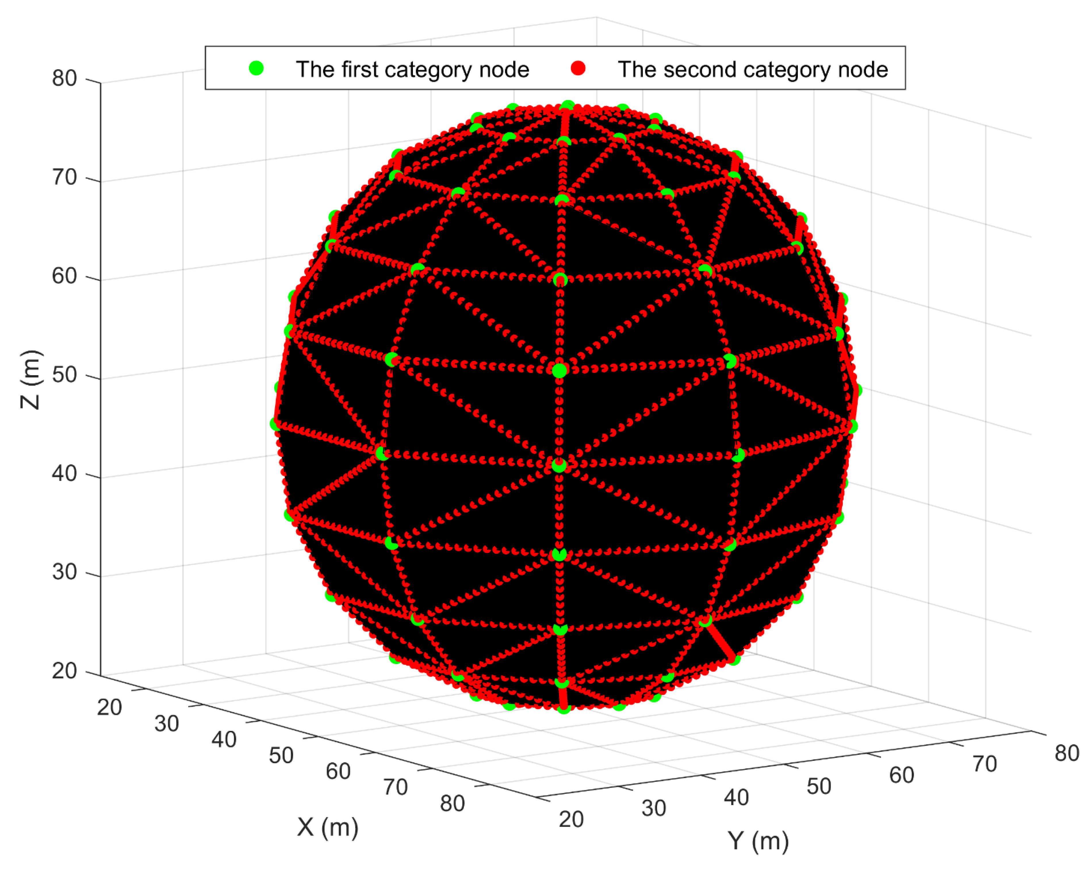
2.2.2. Implementation
- Arrange the second category nodes
- 2.
- Adjacent nodes of each node
- 3.
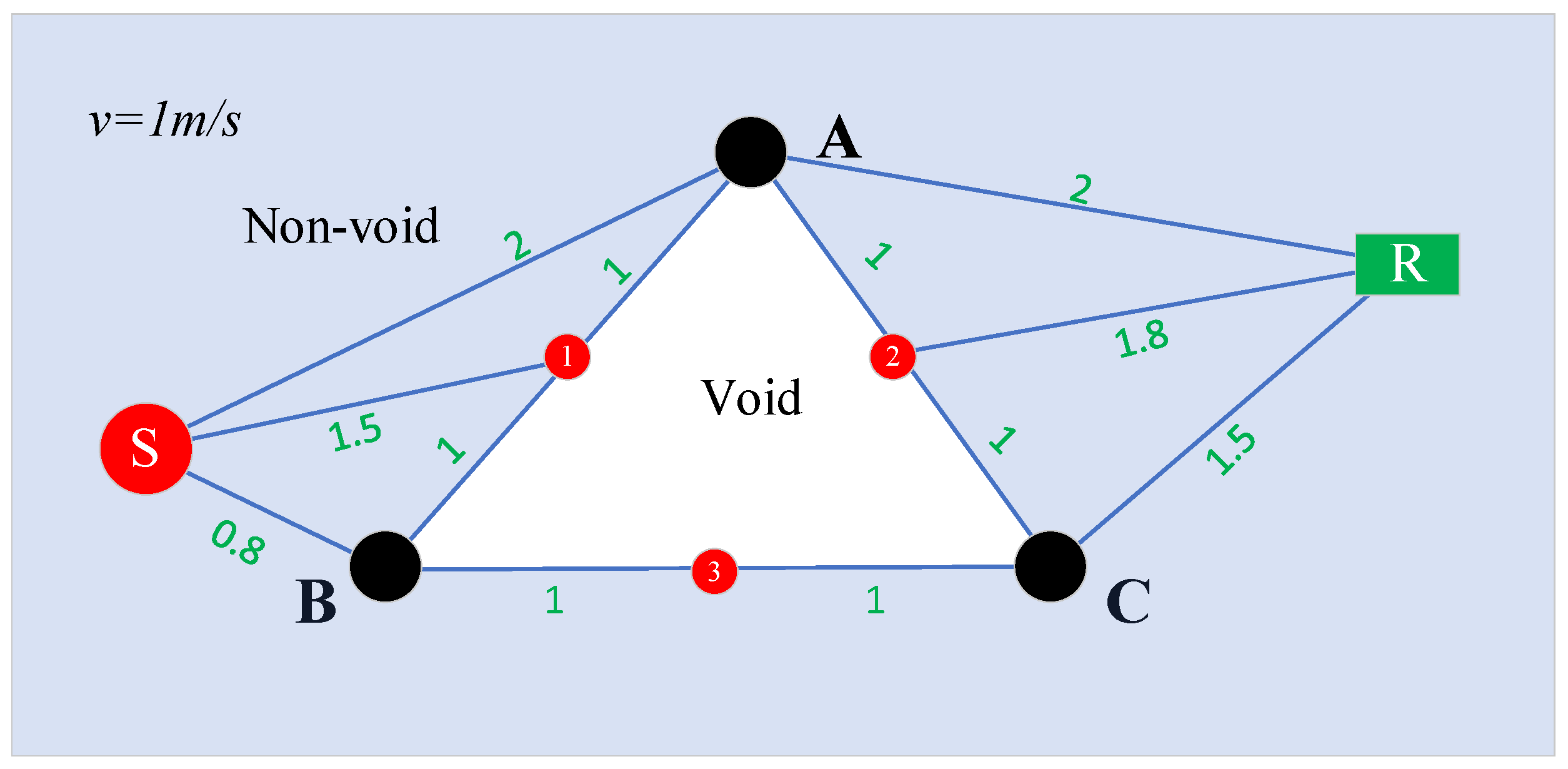
- Ray tracing
3. Synthetic Tests
3.1. Experiments
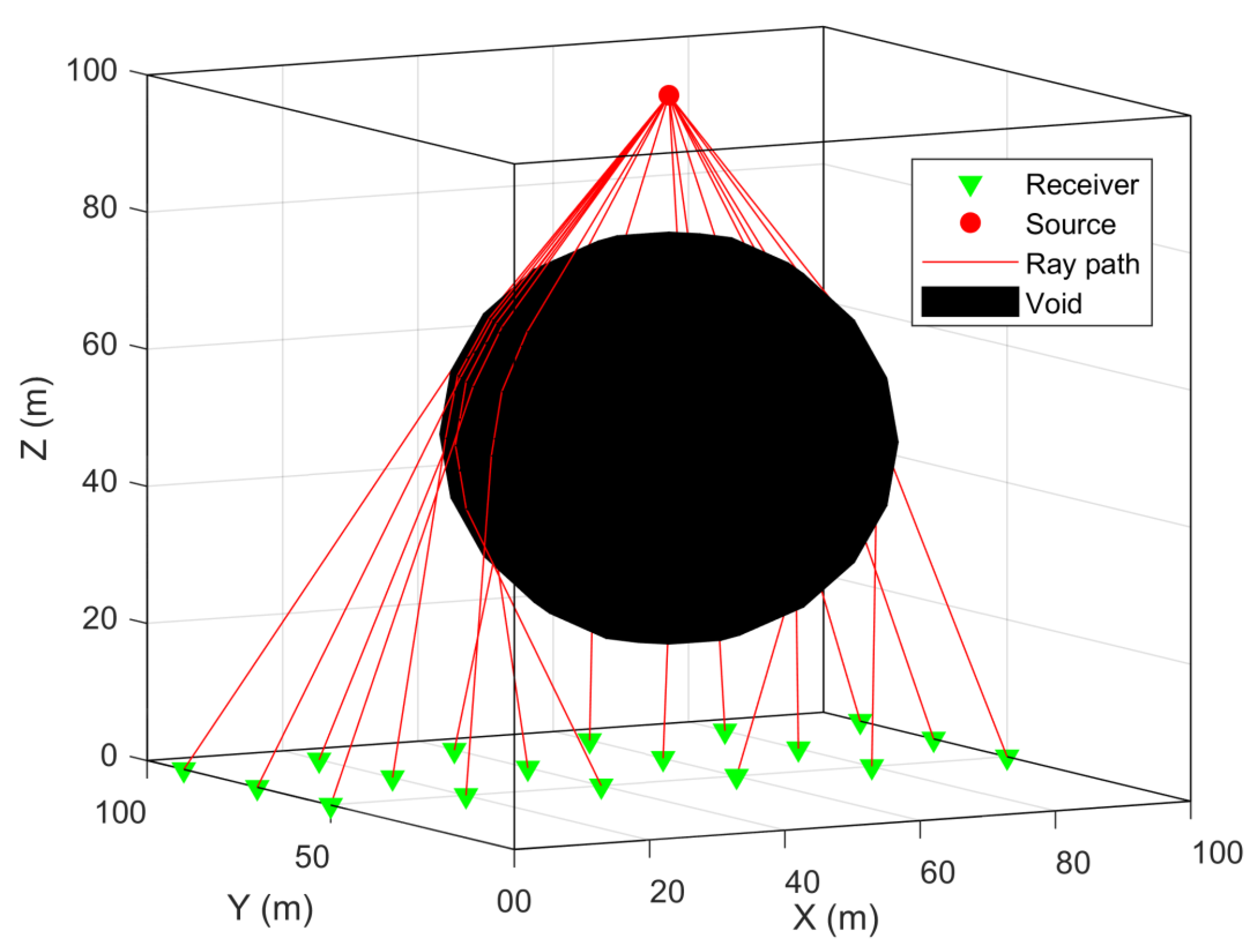
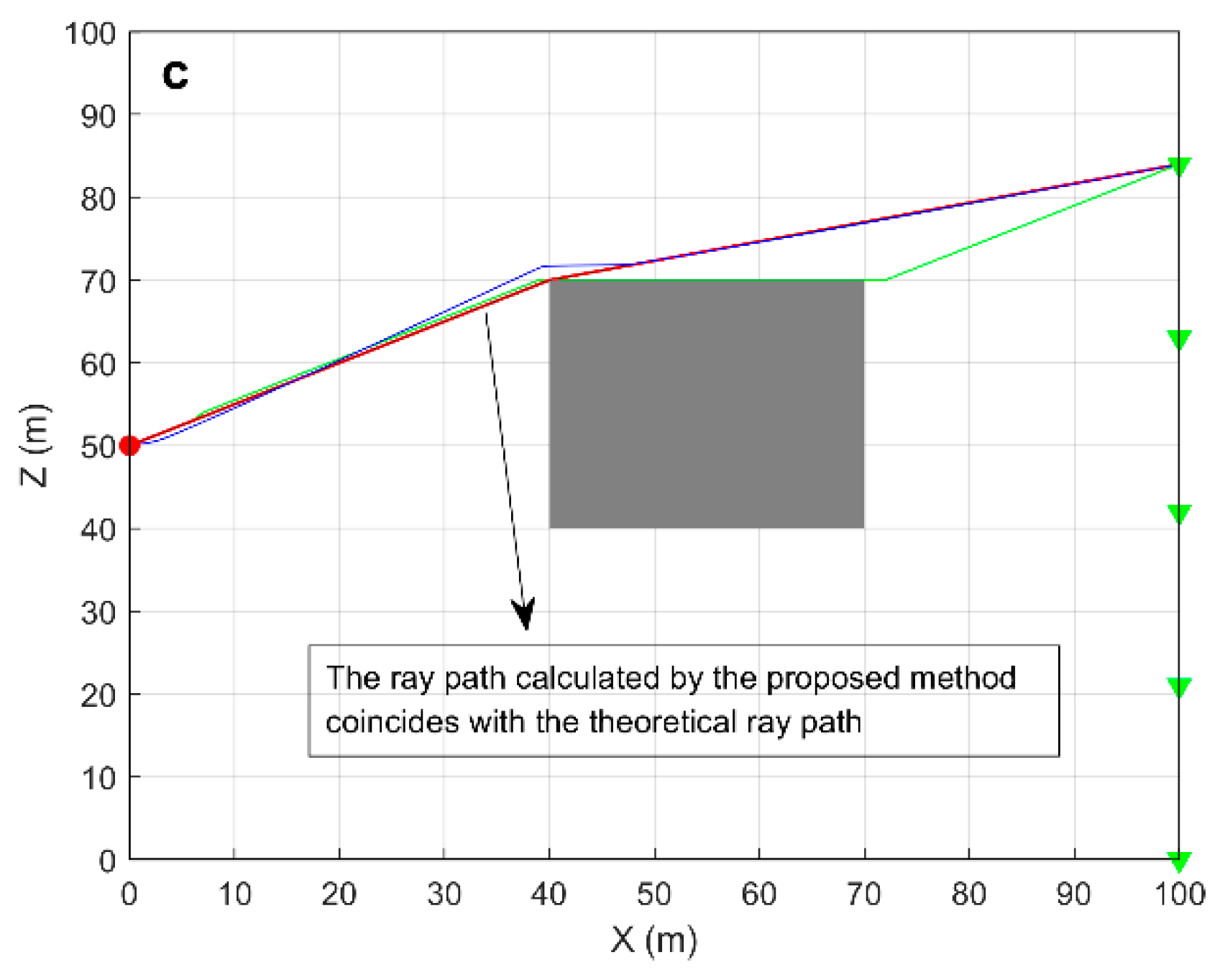
3.1.1. Case 1
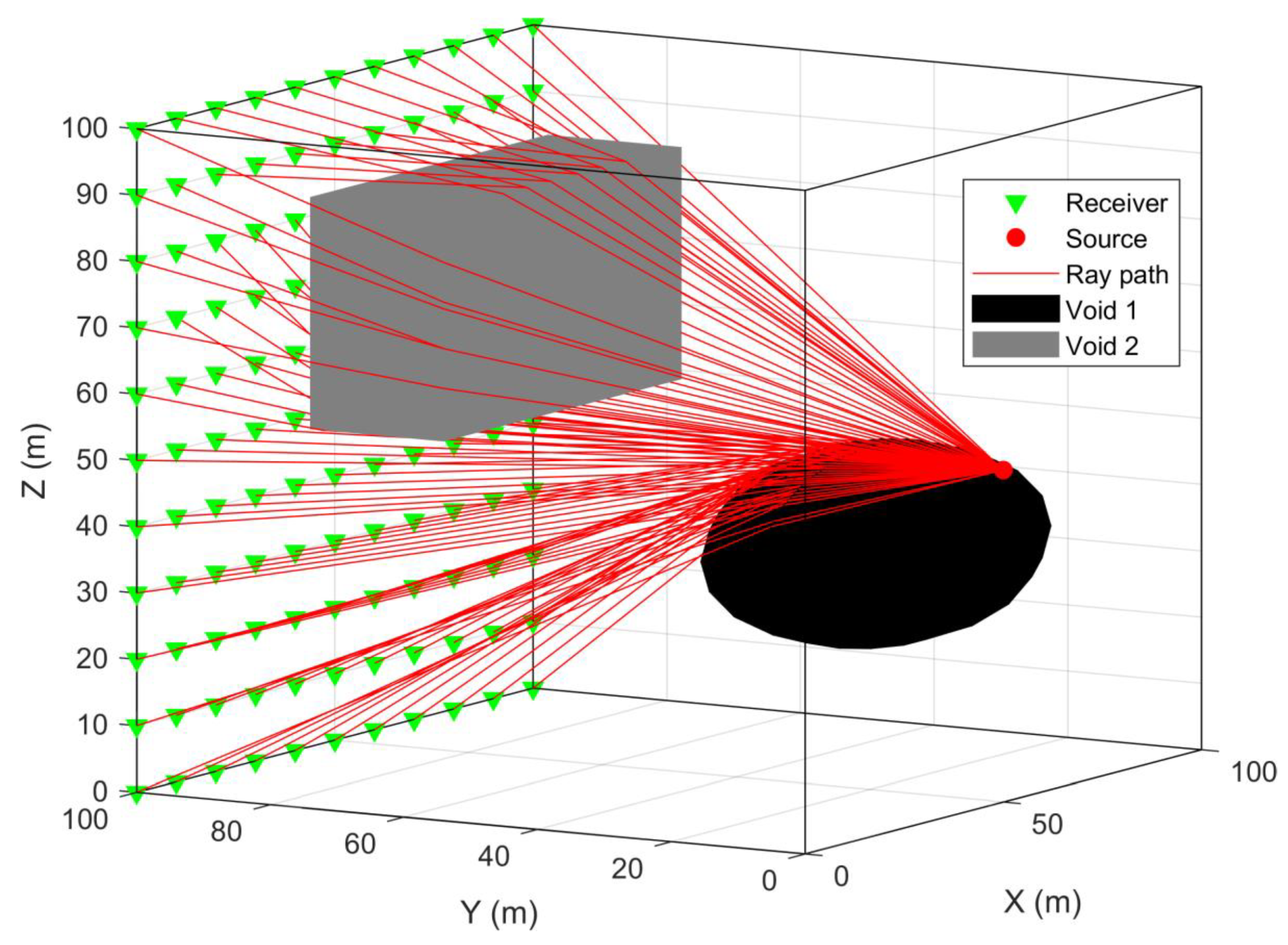
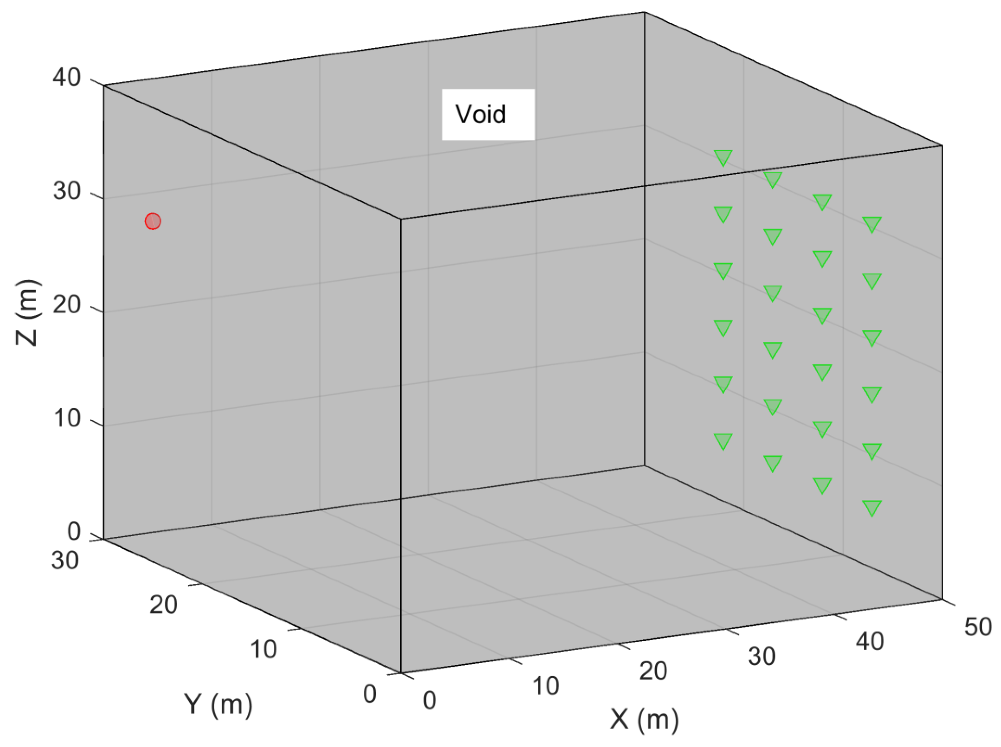
3.1.2. Case 2
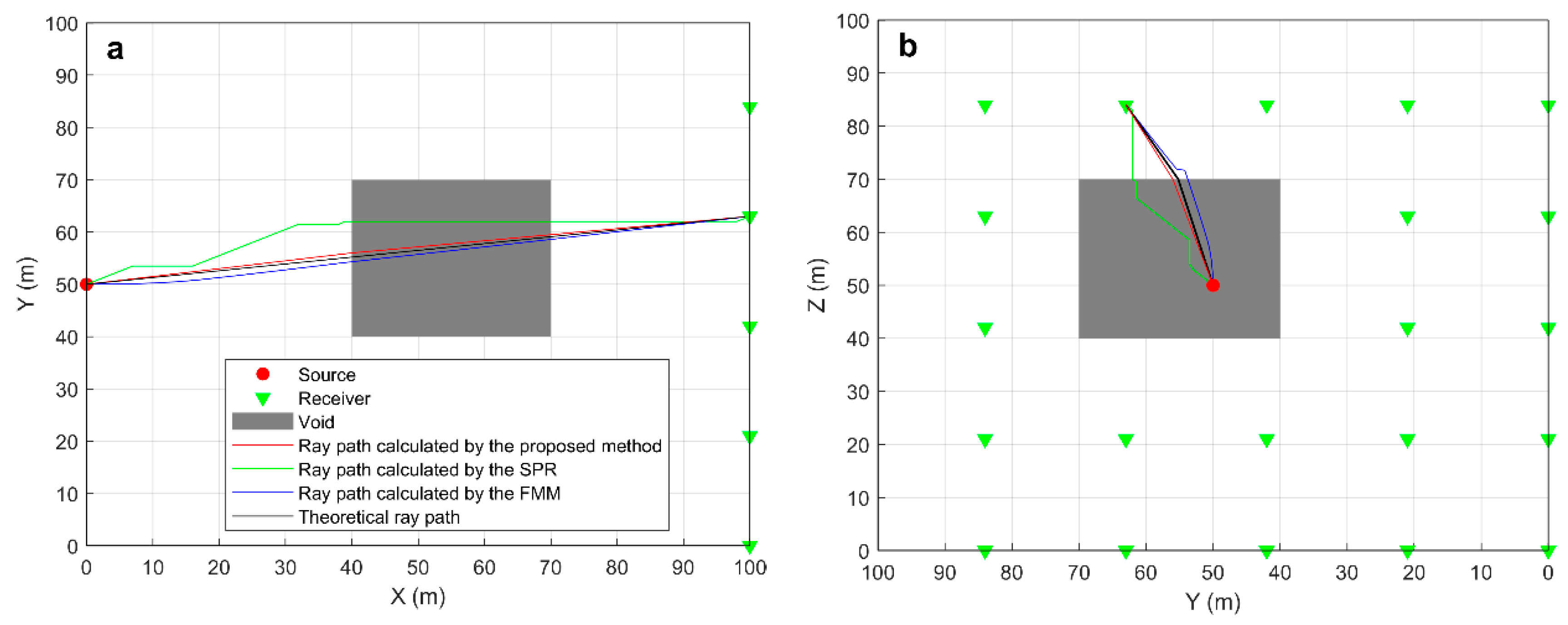
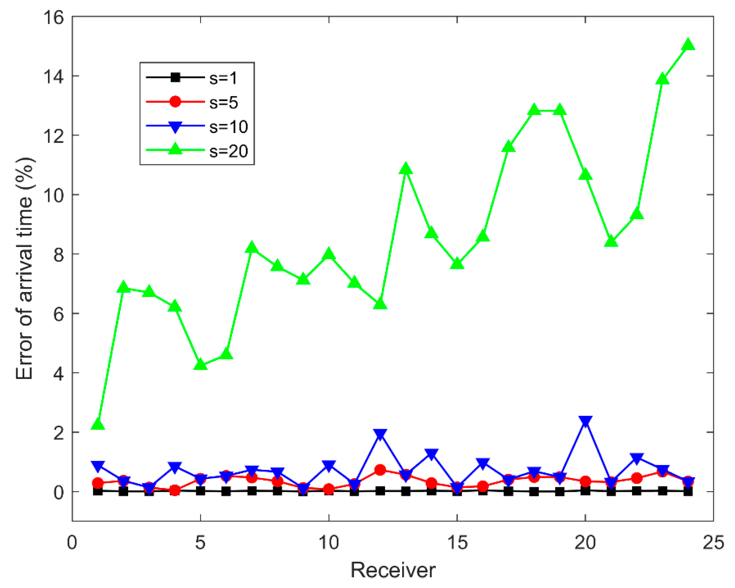
3.2. Comparison and Analysis
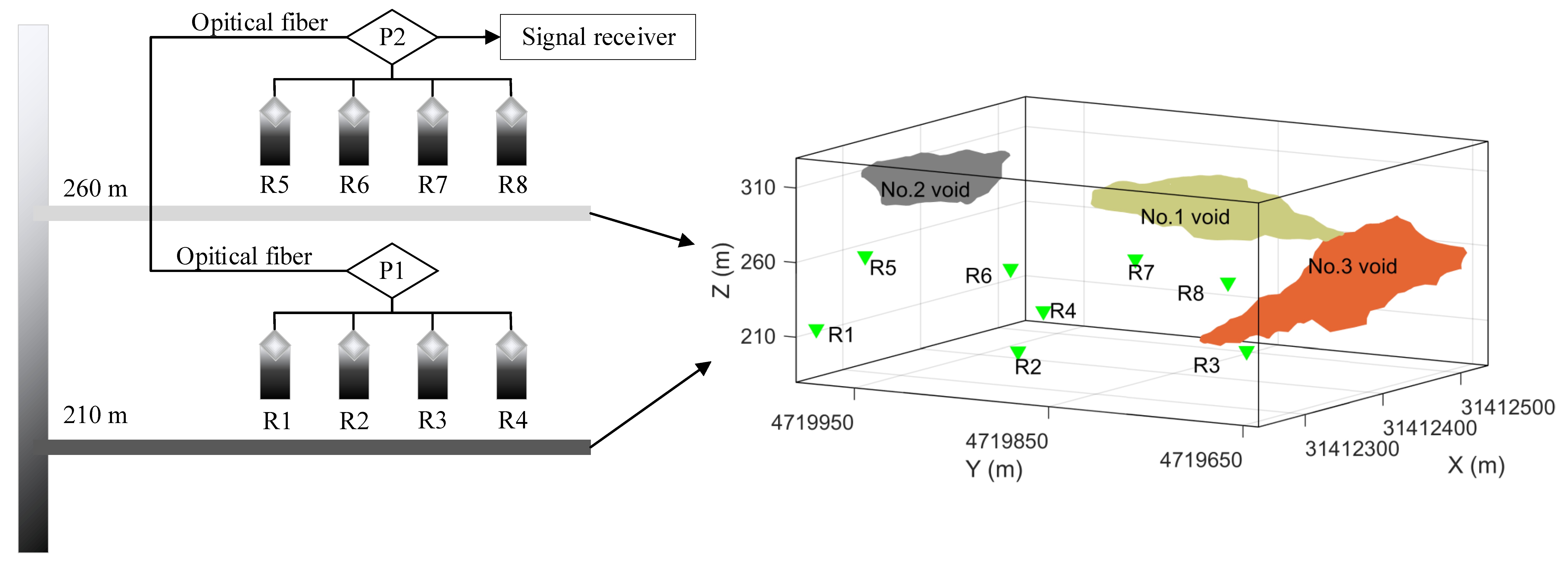
4. Field Application
5. Conclusions
Author Contributions
Funding
Conflicts of Interest
References
- Wang, H.-L.; Ge, M.-C. Acoustic emission/microseismic source location analysis for a limestone mine exhibiting high horizontal stresses. Int. J. Rock Mech. Min. Sci. 2008, 45, 720–728. [Google Scholar] [CrossRef]
- Le Gonidec, Y.; Sarout, J.; Wassermann, J.; Nussbaum, C. Damage initiation and propagation assessed from stress-induced microseismic events during a mine-by test in the Opalinus Clay. Geophys. J. Int. 2014, 198, 126–139. [Google Scholar] [CrossRef]
- Cheng, J.; Song, G.; Sun, X.; Wen, L.; Li, F.; Wena, L.; Li, F.; Wen, L.; Li, F. Research developments and prospects on microseismic source location in mines. Engineering 2018, 4, 653–660. [Google Scholar] [CrossRef]
- Kinscher, J.; Bernard, P.; Contrucci, I.; Mangeney, A.; Piguet, J.P.; Bigarre, P. Location of microseismic swarms induced by salt solution mining. Geophys. J. Int. 2015, 200, 337–362. [Google Scholar] [CrossRef]
- Feng, G.-L.; Feng, X.-T.; Chen, B.-R.; Xiao, Y.-X. Performance and feasibility analysis of two microseismic location methods used in tunnel engineering. Tunn. Undergr. Space Technol. 2017, 63, 183–193. [Google Scholar] [CrossRef]
- Xu, N.W.; Li, T.B.; Dai, F.; Zhang, R.; Tang, C.A.; Tang, L.X. Microseismic monitoring of strainburst activities in deep tunnels at the Jinping II hydropower station, China. Rock Mech. Rock Eng. 2016, 49, 981–1000. [Google Scholar] [CrossRef]
- Feng, G.-L.; Feng, X.-T.; Chen, B.-R.; Xiao, Y.-X.; Jiang, Q. Sectional velocity model for microseismic source location in tunnels. Tunn. Undergr. Space Technol. 2014, 45, 73–83. [Google Scholar] [CrossRef]
- Feng, G.L.; Feng, X.T.; Chen, B.R.; Xiao, Y.X. A highly accurate method of locating microseismic events associated with rockburst development processes in tunnels. IEEE Access 2017, 5, 27722–27731. [Google Scholar] [CrossRef]
- Virieux, J.; Farra, V.; Madariaga, R. Ray tracing for earthquake location in laterally heterogeneous media. J. Geophys. Res. 1988, 93, 6585. [Google Scholar] [CrossRef]
- Zhao, A.-H.; Ding, Z.-F.; Bai, Z.-M. Improvement of the ray-tracing based method for calculating hypocentral Loci for earthquake location. Chin. J. Geophys. 2015, 58, 701–717. [Google Scholar]
- Langan, R.T.; Lerche, I.; Cutler, R.T. Tracing of rays through heterogeneous media: An accurate and efficient procedure. Geophysics 1985, 50, 1456–1465. [Google Scholar] [CrossRef]
- Virieux, J.; Farra, V. Ray tracing in 3-D complex isotropic media: An analysis of the problem. Geophysics 1991, 56, 2057–2069. [Google Scholar] [CrossRef]
- Xu, T.; Zhang, Z.; Zhao, A.; Zhang, A.; Zhang, X.; Zhang, H. Subtriangle shooting ray tracing in complicated 3D VTI media. J. Seism. Explor. 2008, 17, 133–146. [Google Scholar]
- Xu, T.; Xu, G.; Gao, E.; Li, Y.; Jiang, X.; Luo, K. Block modeling and segmentally iterative ray tracing in complex 3D media. Geophysics 2006, 71, T41–T51. [Google Scholar] [CrossRef]
- Um, J.; Thurber, C. A fast algorithm for two-point seismic ray tracing. Bull. Seismol. Soc. Am. 1987, 77, 972–986. [Google Scholar]
- Vinje, V.; Iversen, E.; Gjoystdal, H. Traveltime and amplitude estimation using wavefront construction. Geophysics 1993, 58, 1157–1166. [Google Scholar] [CrossRef]
- Symes, W.W.; Qian, J. A Slowness matching eulerian method for multivalued solutions of eikonal equations. J. Sci. Comput. 2003, 19, 501–526. [Google Scholar] [CrossRef]
- Moser, T.J. Shortest path calculation of seismic rays. Geophysics 1991, 56, 59–67. [Google Scholar] [CrossRef]
- Zhou, B.; Greenhalgh, S.A. “Shortest path” ray tracing for most general 2D/3D anisotropic media. J. Geophys. Eng. 2005, 2, 54–63. [Google Scholar] [CrossRef]
- Bóna, A.; Slawinski, M.A.; Smith, P. Ray tracing by simulated annealing: Bending method. Geophysics 2009, 74, 25–32. [Google Scholar] [CrossRef]
- Sethian, J.A. A fast marching level set method for monotonically advancing fronts. Proc. Natl. Acad. Sci. USA 1996, 93, 1591–1595. [Google Scholar] [CrossRef] [PubMed]
- Hassouna, M.S.; Farag, A.A. Multistencils fast marching methods: A highly accurate solution to the Eikonal equation on Cartesian domains. IEEE Trans. Pattern Anal. Mach. Intell. 2007, 29, 1563–1574. [Google Scholar] [CrossRef] [PubMed]
- Peng, P.; Jiang, Y.; Wang, L.; He, Z. Microseismic event location by considering the influence of the empty area in an excavated tunnel. Sensors 2020, 20, 574. [Google Scholar] [CrossRef] [PubMed]
- Peng, P.; Wang, L. 3DMRT: A computer package for 3D model-based seismic wave propagation. Seismol. Res. Lett. 2019, 90, 2039–2045. [Google Scholar] [CrossRef]
- Peng, P.; Wang, L. Targeted location of microseismic events based on a 3D heterogeneous velocity model in underground mining. PLoS ONE 2019, 14, e0212881. [Google Scholar] [CrossRef] [PubMed]
- Qian, J.; Symes, W.W. An adaptive finite-difference method for traveltimes and amplitudes. Geophysics 2002, 67, 167–176. [Google Scholar] [CrossRef]
- Zhang, L.; Rector, J.W.; Hoversten, G.M. Eikonal solver in the celerity domain. Geophys. J. Int. 2005, 162, 1–8. [Google Scholar] [CrossRef]
- Fomel, S.; Luo, S.; Zhao, H. Fast sweeping method for the factored eikonal equation. J. Comput. Phys. 2009, 228, 6440–6455. [Google Scholar] [CrossRef]
- Noble, M.; Gesret, A.; Belayouni, N. Accurate 3-D finite difference computation of traveltimes in strongly heterogeneous media. Geophys. J. Int. 2014, 199, 1572–1585. [Google Scholar] [CrossRef]
- Zhao, D.; Lei, J. Seismic ray path variations in a 3D global velocity model. Phys. Earth Planet. Inter. 2004, 141, 153–166. [Google Scholar] [CrossRef]
- Jiang, F.; Ye, G.; Wang, C.; Zhang, D.; Guan, Y. Application of high-precision microseismic monitoring technique to water inrush monitoring in coal mine. Chin. J. Rock Mech. Eng. 2008, 27, 1932–1938. [Google Scholar]
- Wang, J.; Jiang, F.; Lu, W.; Wang, C. Microseismic wave propagation velocity insitu experiment and calculation. J. China Coal Soc. 2010, 35, 2059–2063. [Google Scholar]
- Vesnaver, A.L. Ray tracing based on Fermat’s principle in irregular grids. Geophys. Prospect. 1996, 44, 741–760. [Google Scholar] [CrossRef]
- Zhang, M.; Xu, T.; Bai, Z.; Liu, Y.; Hou, J.; Yu, G. Ray tracing of turning wave in elliptically anisotropic media with an irregular surface. Earthq. Sci. 2017, 30, 219–228. [Google Scholar] [CrossRef]


| R1 | R2 | R3 | R4 | R5 | R6 | R7 | R8 | R9 | ||
|---|---|---|---|---|---|---|---|---|---|---|
| x (m) | 100 | 100 | 100 | 100 | 100 | 100 | 100 | 100 | 100 | |
| y (m) | 0 | 0 | 0 | 0 | 0 | 21 | 21 | 21 | 21 | |
| z (m) | 0 | 21 | 42 | 63 | 84 | 0 | 21 | 42 | 63 | |
| Travel time (ms) | Proposed method | 24.50 | 23.10 | 22.42 | 22.51 | 23.37 | 23.10 | 21.62 | 20.89 | 20.99 |
| FMM | 24.55 | 23.16 | 22.46 | 22.56 | 23.43 | 23.16 | 21.67 | 20.93 | 21.03 | |
| SPR | 24.49 | 23.60 | 22.70 | 22.92 | 23.81 | 23.60 | 22.61 | 21.71 | 21.92 | |
| R10 | R11 | R12 | R13 | R14 | R15 | R16 | R17 | R18 | ||
| x (m) | 100 | 100 | 100 | 100 | 100 | 100 | 100 | 100 | 100 | |
| y (m) | 21 | 42 | 42 | 42 | 42 | 42 | 63 | 63 | 63 | |
| z (m) | 84 | 0 | 21 | 42 | 63 | 84 | 0 | 21 | 42 | |
| Travel time (ms) | Proposed method | 21.91 | 22.42 | 20.89 | 20.32 | 20.43 | 21.33 | 22.51 | 20.99 | 20.43 |
| FMM | 21.97 | 22.46 | 20.93 | 20.71 | 20.61 | 21.49 | 22.56 | 21.03 | 20.61 | |
| SPR | 22.84 | 22.70 | 21.71 | 21.00 | 21.22 | 21.98 | 22.92 | 21.92 | 21.22 | |
| R19 | R20 | R21 | R22 | R23 | R24 | R25 | ||||
| x (m) | 100 | 100 | 100 | 100 | 100 | 100 | 100 | |||
| y (m) | 63 | 63 | 84 | 84 | 84 | 84 | 84 | |||
| z (m) | 63 | 84 | 0 | 21 | 42 | 63 | 84 | |||
| Travel time (ms) | Proposed method | 21.27 | 21.43 | 23.37 | 21.91 | 21.33 | 21.43 | 22.33 | ||
| FMM | 22.83 | 21.59 | 23.43 | 21.97 | 21.49 | 21.59 | 22.68 | |||
| SPR | 21.86 | 22.19 | 23.81 | 22.84 | 21.98 | 22.19 | 23.09 | |||
| x (m) | y (m) | z (m) | Arrival Time (ms) | |||||
|---|---|---|---|---|---|---|---|---|
| Theory | s = 1 | s = 5 | s = 10 | s = 20 | ||||
| S | 0 | 25 | 30 | 0 | 0 | 0 | 0 | 0 |
| R1 | 50 | 7 | 7 | 16.27 | 16.31 | 16.41 | 16.63 | 19.72 |
| R2 | 50 | 7 | 12 | 16.01 | 16.07 | 16.07 | 17.11 | 19.48 |
| R3 | 50 | 7 | 17 | 15.82 | 15.84 | 15.84 | 16.87 | 18.71 |
| R4 | 50 | 7 | 22 | 15.69 | 15.69 | 15.82 | 16.66 | 17.76 |
| R5 | 50 | 7 | 27 | 15.04 | 15.10 | 15.10 | 15.67 | 16.85 |
| R6 | 50 | 7 | 32 | 14.07 | 14.14 | 14.14 | 14.72 | 16.02 |
| R7 | 50 | 12 | 7 | 15.31 | 15.38 | 15.42 | 16.56 | 18.90 |
| R8 | 50 | 12 | 12 | 15.04 | 15.09 | 15.14 | 16.18 | 18.89 |
| R9 | 50 | 12 | 17 | 14.83 | 14.85 | 14.85 | 15.89 | 18.08 |
| R10 | 50 | 12 | 22 | 14.69 | 14.70 | 14.82 | 15.86 | 17.33 |
| R11 | 50 | 12 | 27 | 14.61 | 14.65 | 14.65 | 15.64 | 16.68 |
| R12 | 50 | 12 | 32 | 13.79 | 13.89 | 14.06 | 14.66 | 16.18 |
| R13 | 50 | 17 | 7 | 14.36 | 14.44 | 14.44 | 15.91 | 18.00 |
| R14 | 50 | 17 | 12 | 14.07 | 14.11 | 14.25 | 15.29 | 18.41 |
| R15 | 50 | 17 | 17 | 13.85 | 13.87 | 13.87 | 14.90 | 17.52 |
| R16 | 50 | 17 | 22 | 13.70 | 13.72 | 13.83 | 14.87 | 16.68 |
| R17 | 50 | 17 | 27 | 13.62 | 13.67 | 13.67 | 15.19 | 15.91 |
| R18 | 50 | 17 | 32 | 13.41 | 13.48 | 13.51 | 15.13 | 15.29 |
| R19 | 50 | 22 | 7 | 13.41 | 13.48 | 13.48 | 15.13 | 17.17 |
| R20 | 50 | 22 | 12 | 13.11 | 13.15 | 13.42 | 14.50 | 17.93 |
| R21 | 50 | 22 | 17 | 12.87 | 12.91 | 12.91 | 13.94 | 17.11 |
| R22 | 50 | 22 | 22 | 12.70 | 12.76 | 12.85 | 13.89 | 16.18 |
| R23 | 50 | 22 | 27 | 12.62 | 12.70 | 12.71 | 14.36 | 15.29 |
| R24 | 50 | 22 | 32 | 12.61 | 12.65 | 12.65 | 14.50 | 14.50 |
| Accuracy | Effectiveness | Grid | Scope of Application | |
|---|---|---|---|---|
| Proposed method | High | Fast | No | Underground mine with a lot of voids and the wave velocity in the non-voids is not much different. |
| FMM | Higher | Faster | Yes | All fields |
| SPR | low | slow | Yes | All fields |
| Blasts | B1 | B2 | B3 | Mean | |
|---|---|---|---|---|---|
| Actual position | x (m) | 31,412,506.50 | 31,412,516.92 | 31,412,514.32 | |
| y (m) | 4,719,746.39 | 4,719,743.59 | 4,719,815.21 | ||
| z (m) | 146.68 | 119.19 | 134.94 | ||
| Location method with constant velocity | x (m) | 31,412,512.19 | 31,412,531.62 | 31,412,533.47 | |
| y (m) | 4,719,758.60 | 4,719,726.15 | 4,719,802.70 | ||
| z (m) | 137.57 | 127.94 | 146.69 | ||
| Location error (m) | 16.26 | 24.44 | 25.72 | 22.14 | |
| Location method based on FMM | x (m) | 31,412,509.44 | 31,412,511.35 | 31,412,521.42 | |
| y (m) | 4,719,749.60 | 4,719,749.67 | 4,719,813.89 | ||
| z (m) | 143.57 | 122.49 | 136.74 | ||
| Location error (m) | 5.35 | 8.87 | 7.44 | 7.22 | |
| Location method based on the proposed ray tracing | x (m) | 31,412,508.98 | 31,412,520.52 | 31,412,517.76 | |
| y (m) | 4,719,743.05 | 4,719,746.21 | 4,719,818.79 | ||
| z (m) | 149.03 | 114.29 | 131.16 | ||
| Location error (m) | 4.78 | 6.62 | 6.24 | 5.88 | |
© 2020 by the authors. Licensee MDPI, Basel, Switzerland. This article is an open access article distributed under the terms and conditions of the Creative Commons Attribution (CC BY) license (http://creativecommons.org/licenses/by/4.0/).
Share and Cite
Peng, P.; Jiang, Y.; Wang, L.; He, Z.; Tu, S. A Fast Ray-tracing Method for Locating Mining-Induced Seismicity by Considering Underground Voids. Appl. Sci. 2020, 10, 6763. https://doi.org/10.3390/app10196763
Peng P, Jiang Y, Wang L, He Z, Tu S. A Fast Ray-tracing Method for Locating Mining-Induced Seismicity by Considering Underground Voids. Applied Sciences. 2020; 10(19):6763. https://doi.org/10.3390/app10196763
Chicago/Turabian StylePeng, Pingan, Yuanjian Jiang, Liguan Wang, Zhengxiang He, and Siyu Tu. 2020. "A Fast Ray-tracing Method for Locating Mining-Induced Seismicity by Considering Underground Voids" Applied Sciences 10, no. 19: 6763. https://doi.org/10.3390/app10196763
APA StylePeng, P., Jiang, Y., Wang, L., He, Z., & Tu, S. (2020). A Fast Ray-tracing Method for Locating Mining-Induced Seismicity by Considering Underground Voids. Applied Sciences, 10(19), 6763. https://doi.org/10.3390/app10196763