Simulation-Based Assessment of the Operational Performance of the Finnish–Swedish Winter Navigation System

Abstract

This article presents a discrete event simulation-based approach for assessing the operating performance of the Finnish–Swedish Winter Navigation System (FSWNS) under different operating scenarios. Different operating scenarios are specified in terms of ice conditions, the volume of maritime traffic, number of icebreakers (IBs), and regulations such as the Energy Efficiency Design Index (EEDI). Considered performance indicators include transport capacity, number of instances of icebreaker (IB) assistance, and IB waiting times. The approach is validated against real-world data on maritime traffic in the Bothnian Bay. In terms of the number of ship arrivals per port, indicating the transport capacity of the FSWNS, the simulation agrees well with the data. In terms of the number of instances of IB assistance and IB waiting times per port, the standard deviations between the mean of 35 independent simulation runs and the data are 13% and 18%, respectively. A sensitivity analysis indicates that the simulated number of instances of IB assistance and IB waiting times is particularly sensitive to assumptions concerning the presence of brash ice channels. Case studies indicate that, unless the number of IBs is increased, the EEDI regulations may result in a significant increase in both the number of instances of IB assistance and the cumulated IB waiting times.

1. Introduction

The Baltic Sea is an important transit route connecting numerous countries and markets. In 2019, the total volume of Finnish import and export transported over the Baltic Sea exceeded 100 million tons, corresponding to around 80% of the total trade [1,2]. These numbers are expected to increase as the long-term trend in the volume of Finnish seaborne trade is one of growth [3].

In winter, large parts of the Baltic Sea are typically ice-covered, but with significant interannual variability with regards to the maximum ice extent [4]. This variability poses a challenge to shipping in the region, as sea ice has a significant impact on the operations and transit times of ships. The aim of the Finnish–Swedish Winter Navigation System (FSWNS) is to maintain safe and efficient year-round navigation to and from Finnish and Swedish ports along the Baltic Sea [5]. To this end, the FSWNS manages winter navigation-related challenges by the combined use of (a) ice class rules, (b) traffic regulations, and (c) icebreaker (IB) assistance [6]. Specifically, to make sure that ships have enough ice-going capability for safe and efficient operations, they must be built and operated following the Finnish–Swedish Ice Class Rules (FSICR) [5]. These are enforced by port-specific traffic restrictions set by Finnish and Swedish maritime authorities in terms of the minimum ice class and deadweight needed to be eligible for IB assistance [5]. IB assistance is provided based on the available fleet of Finnish and Swedish state-owned and operated IBs. As per [7,8], Finland has a fleet of eight major IBs (Polaris, Fennica, Nordica, Otso, Kontio, Voima, Sisu, and Urho), whereas Sweden has a fleet of five major IBs (Ale, Atle, Frej, Oden, and Ymer).

Both in the short- and longer-term, the performance of the FSWNS is expected to be influenced by the International Maritime Organization’s (IMO) Energy Efficiency Design Index (EEDI) regulations. These regulations, which were adopted by the IMO in July 2011, aim to reduce the amount of greenhouse gasses (GHGs) from ships by promoting the use of more energy-efficient solutions [9]. Anyhow, due to the technical content of the regulations, they are expected to limit the installed propulsion power of ships, which will reduce their ice-going capability and attainable speed in ice. This in turn could increase the demand for IB assistance, resulting in more frequent and longer waiting times for IB assistance, which is expected to increase the overall transport costs and time.

Towards assessing the influence of the EEDI, and to identify and assess possible mitigation measures, this article presents an approach for assessing the operational performance of the FSWNS under various operating condition scenarios. The approach builds on a discrete event simulation (DES)-based approach presented by [10]. DES is a specific type of simulation in which the behavior of a system is modelled as an ordered sequence of events, each of which takes place at a specific point of time and results in a change in the state of the system [11]. As no change occurs between events, DES enables fast simulations of extensive operating periods. Additionally, as individual events can be modelled so that they are dependent on stochastic variables, DES is well suited to considering uncertainties and stochastic factors. In addition, because DES makes it possible to model individual ships as entities moving through a system in the manner of a queue, the technique is well suited to capturing various interactions and self-reinforcing effects.

The approach presented by [10] can assess the performance of an Arctic maritime transport system consisting of a homogenous fleet of ships operating between two ports. In this study, the approach is extended to handle the significantly more complex operations of the FSWNS. Related research questions include the following: Is it feasible to capture the complex behavior and to roughly estimate the operating performance of the FSWNS using a DES-based approach? What behaviors of the FSWNS are difficult to capture using DES? What are the future research needs?

Other approaches to simulate the FSWNS include [12], in which the transport system is simulated using a brute-force optimization-based approach, providing a good agreement with real-world data. A potential weakness of [12] is that its application appears to be laborious and time-consuming due to its mathematical nature. Furthermore, as the approach [12] appears not to be based on ship entities, it is unclear how it handles various interaction and self-reinforcing behaviors of the FSWNS (e.g., if a ship arrives late at a port, it should also leave the port late), which might be significant in an extreme scenario.

2. Background

2.1. Finnish–Swedish Ice Class Rules and IB Waiting Time

The aim of the Finnish–Swedish Ice Class Rules (FSICR) is to ensure that ships operating on the northern Baltic Sea, to and from Finnish and Swedish ports, have sufficient ice-going capability to maintain safe and efficient navigation year-round [13]. To this end, the rules, which have been developed jointly by the Finnish and Swedish maritime authorities based on accumulated experience and research, specify five ice classes: IA Super, IA, IB, IC, and II. Enforcement is through port-specific restrictions determining the minimum ice class and deadweight needed to be eligible for IB assistance [13].

The demand for IB assistance in a region depends among others on the prevailing ice conditions, the amount of maritime traffic, and the ice-going capability of the ships operating there. If the demand for IB assistance exceeds the available icebreaking resources, the waiting time for IB assistance will increase. To maintain smooth and efficient maritime traffic, the goal of the Finnish IB service is to limit the average waiting time to four hours [14]. To this end, the FSICR determines ice class-specific performance requirements. These are determined as per [5] in terms of the minimum ice conditions in which a ship must be able to maintain a speed of at least 5 knots.

2.2. Energy Efficiency Design Index (EEDI)

The EEDI regulations regulate a ship’s $\mathrm{C}{\mathrm{O}}_2$ emissions by specifying its maximum allowed EEDI value determined as a function of deadweight tonnage (DWT) or gross tonnage (GT), separately for different types of ships (e.g., bulk carriers, tankers, gas carriers, roll-on/roll-off cargo ships) [15]. To stimulate continued innovation and technical development, the maximum allowed EEDI will be tightened incrementally every five years [9].

In simplified terms, the EEDI value represents the amount of $\mathrm{C}{\mathrm{O}}_2$ generated by a ship carrying out a specific transport work [15]. Accordingly, the EEDI value can be expressed as per Equation (1) based on engine power, specific fuel consumption (SFC), an assumed amount of $\mathrm{C}{\mathrm{O}}_2$ per gram of fuel (${\mathrm{C}}_{\mathrm{F}}$), DWT, and ship speed [16].

$$\mathrm{EEDI}=\frac{\mathrm{C}{\mathrm{O}}_2\mathrm{emissions}}{\mathrm{transport\; work}}=\frac{\mathrm{Engine\; power}\ast {\mathrm{C}}_{\mathrm{F}}}{\mathrm{DWT}\ast \mathrm{speed}}$$

(1)

As per Equation (1), for a given type of engine and fuel, the EEDI regulations effectively limit the maximum installed propulsion power. To make ice-class ships comparable with open water ships, considering that they need extra propulsion power for operation in ice, the EEDI regulations include correction factors [17]. These are determined for five different types of ships: tanker, bulk, general cargo, container, gas carriers, and roll-on/roll-off ships [17]. Notwithstanding, the EEDI regulations are expected to reduce the average propulsion power, and consequently also the average ice-going capability of ice classed ships. This implies a reduction in both the maximum ice conditions in which ships can operate independently and the speed of ships in ice. For a given operating scenario, this will increase both the number of instances where a ship needs IB assistance and the duration of each instance of IB assistance. As a result, the demand for IB assistance is expected to increase [18]. Additionally, considering the maritime industry’s overall efforts to optimize maritime operations, the demand for IB assistance might also be driven by non-EEDI-related cost and energy consumption reducing measures, further reducing the ice-going capability of ships.

3. Description of the Simulation Model

3.1. Programming Platform

The proposed simulation approach is implemented in MATLAB (ver. R2020a), using its discrete event simulation tool SimEvents (based on SimuLink ver. 10.1/ R2020a). As per [19], SimEvents provides a discrete-event simulation engine and component library for analyzing event-driven system models and optimizing performance characteristics. A set of predefined blocks, including queues, servers, switches, supports the modelling work.

3.2. Model Structure and Working Principle

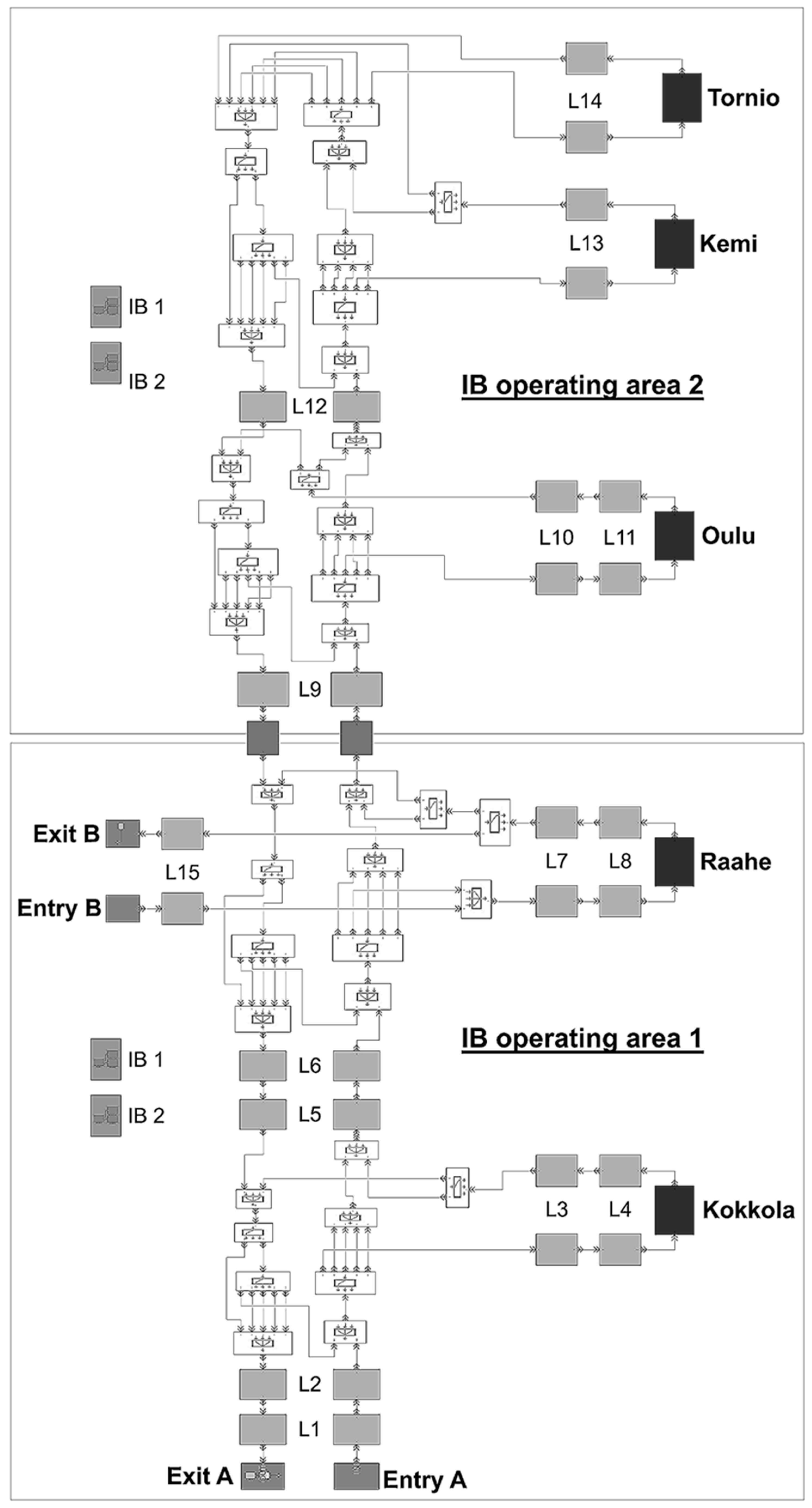
As per Figure 1 presenting an example simulation model structure, the simulation model consists of different types of blocks representing navigation legs (L), ports, crossings, borders between different IB operating areas, and ship entry/exit gates. Ships are represented by entities, each of which has a set of predetermined attributes specifying the technical characteristics (e.g., ice-going capability) and voyage characteristics (destination ports, port-turnaround times) of the ship. IBs, on the other hand, are represented by “resources”. Specifically, an individual IB is represented by an individual IB resource that, when assisting a ship, is attached to the ship being assisted.

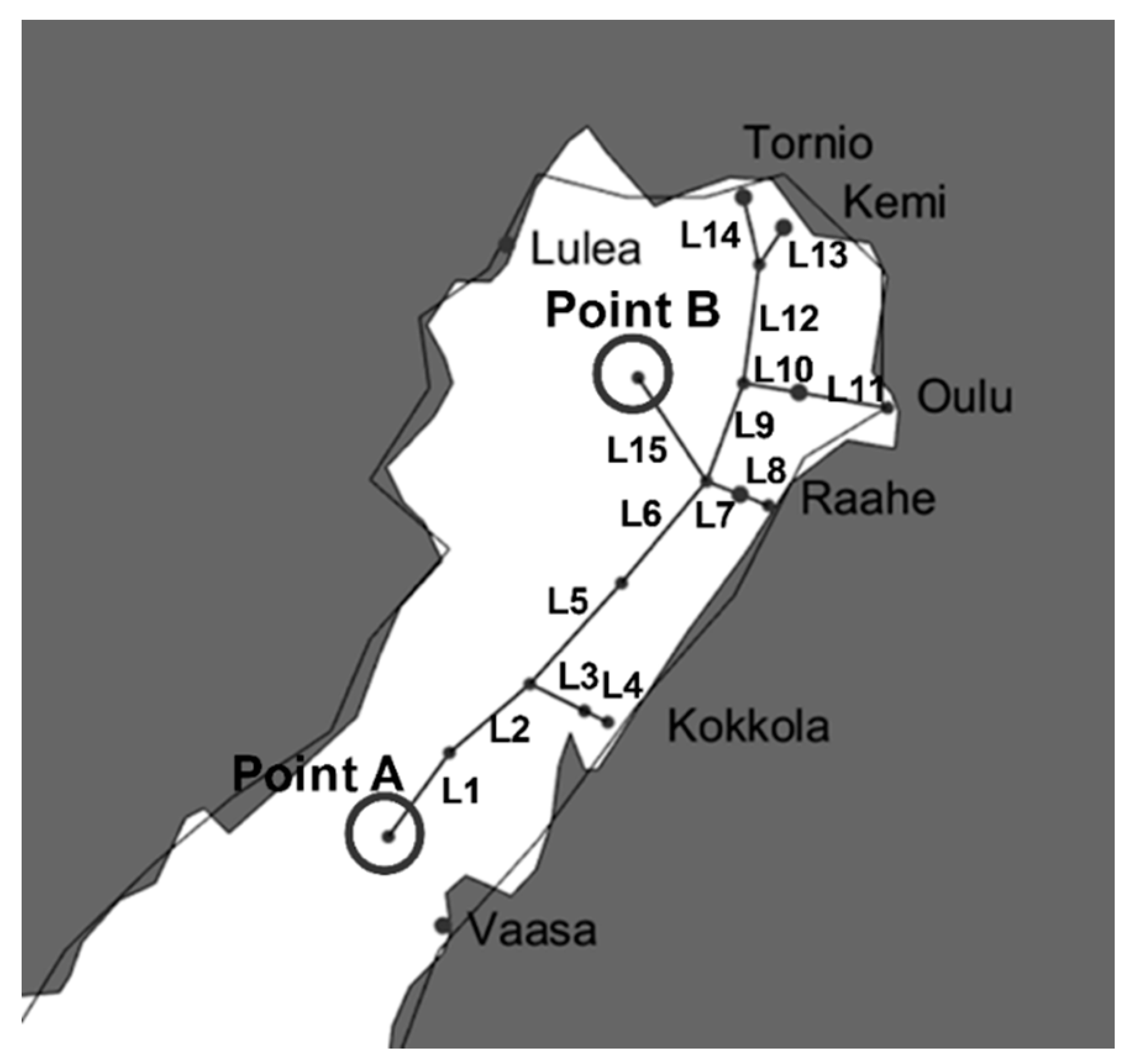
Each ship entity enters the simulation model at a specific date and time (determined based on maritime traffic data) through an entry gate with an assumed geographical location (e.g., Kvarken, Bay of Bothnia). Once entered, a ship entity will progress towards its first port of destination, where it will stay for a predetermined period corresponding to the total port turnaround time. Thereafter, the ship entity will either continue towards another port within the simulation model or towards a port located outside the simulation model. In the latter case, the ship entity will progress towards an exit gate with an assumed geographical location and then leave the simulation model.

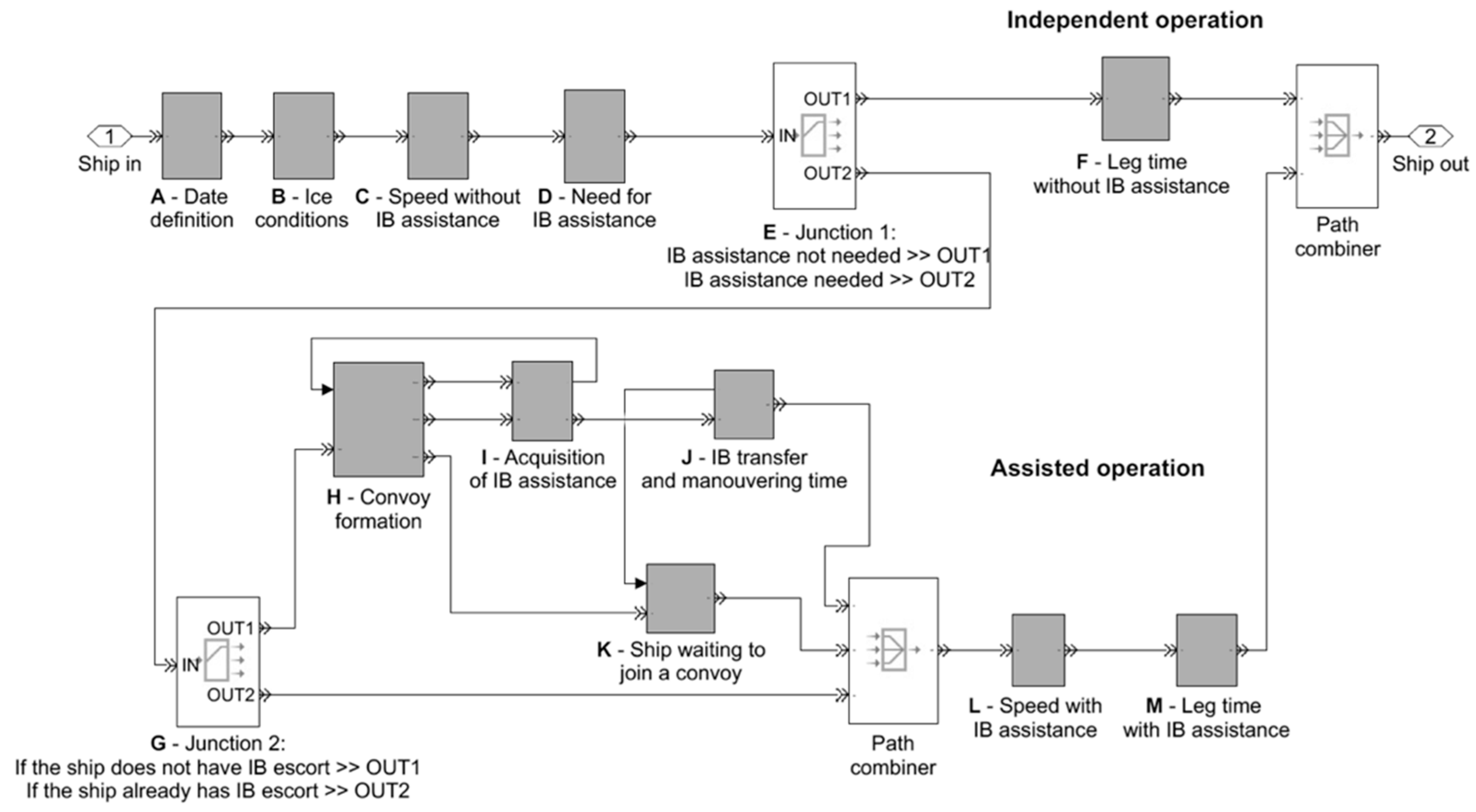
Navigation legs are here defined as the geographical distance between two waypoints. The time it takes for a ship entity to complete a leg depends on the leg distance, the ice conditions, the operating mode (independent or assisted operation), the ship’s estimated speed in the prevailing ice conditions and operating mode, and the waiting time for IB assistance (in case the ship must call for IB assistance). Specifically, navigation legs are modelled as per the schematic diagram in Figure 2 whose various elements are described as follows:

• A—Date definition. When a ship entity (with or without IB assistance) arrives at a waypoint, the present date is determined in terms of the number of days elapsed since the start of the simulation.
• B—Ice conditions. The prevailing ice conditions are determined following a predefined table defining the ice conditions by navigation leg and date. The prevailing ice thickness along the leg is defined in terms of the average equivalent ice thickness ($H_{eq\_avg}$) (cm) and the maximum equivalent ice thickness ($H_{eq\_max}$) (cm). $H_{eq\_avg}$ is defined as the average thickness of all major ice features (level ice, ice ridges, openings) over the whole leg. $H_{eq\_max}$, in turn, is defined as the average thickness of the same ice features over the part of the leg with the most difficult ice conditions (e.g., an area with severe ice ridging). In order to account for uncertainty and stochasticity, during an individual simulation run the applied $H_{eq\_avg}$ and $H_{eq\_max}$ values are multiplied by randomly determined coefficients representing their uncertainty. In addition, based on the location and prevailing ice conditions, an assumption is made as to whether a brash ice channel is present. Specifically, depending on the location of a leg and the prevailing ice conditions there, a brash ice channel is assumed to be (a) present at all times, (b) present with a certain probability, or (c) never present. If an ice channel is assumed present with a certain probability, whether an ice channel is present at a specific date is determined based on a binary number (0 = no ice channel, 1 = ice channel) drawn from an assumed distribution.
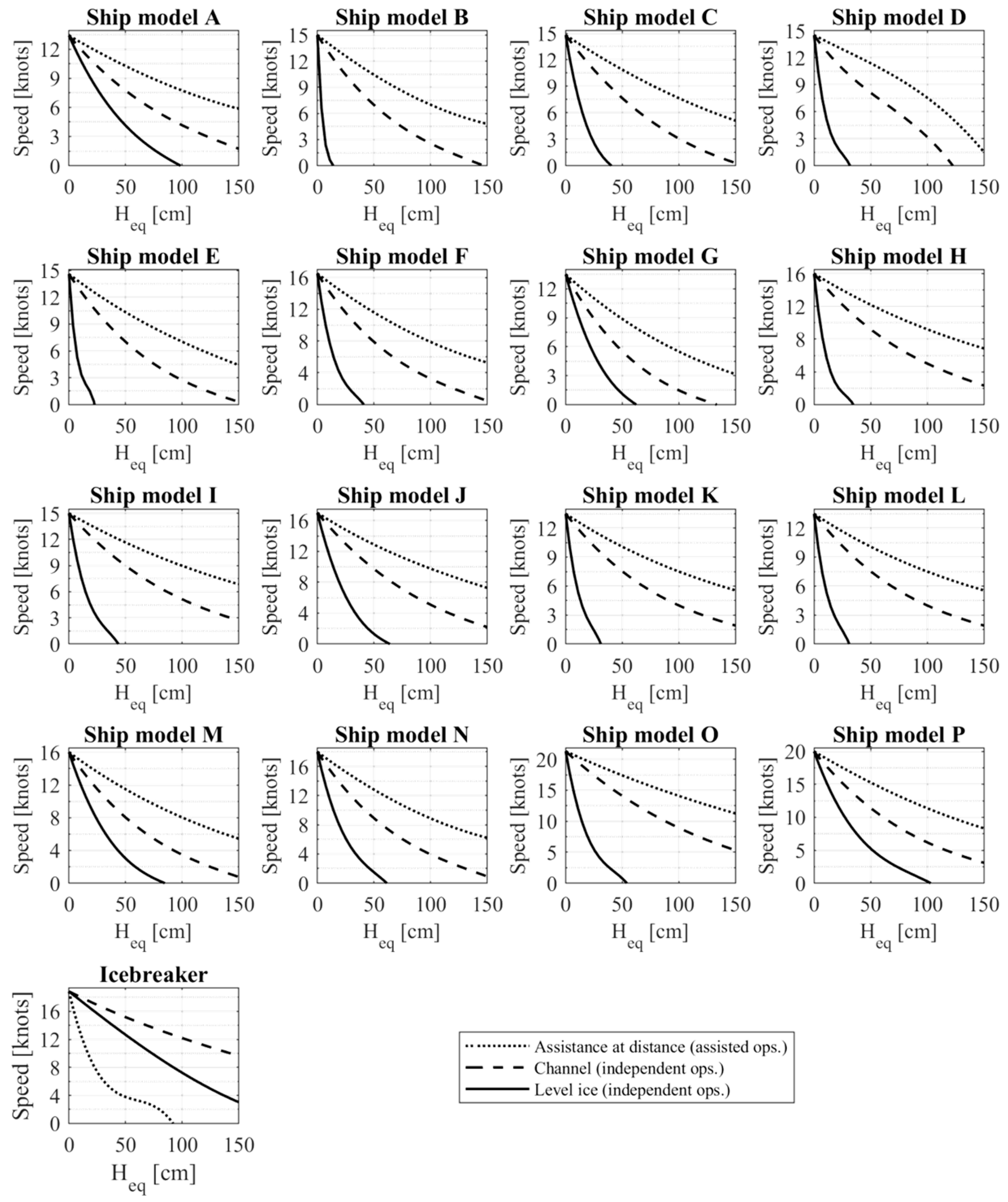
• C—Speed without IB assistance. The assumed independently achievable speed (knots) of a vessel is determined both for $H_{eq\_avg}$ and $H_{eq\_max}$ based on ship and operation type-specific hv curves that determine the speed of a ship as a function of the ice thickness. As per the example hv curves presented in Figure 3, two different types of independent operation are considered:

  ∘

  Independent operation in a brash ice channel (“Channel” as per Figure 3). Here, the ship is operating in a pre-existing brash ice channel without IB assistance. Ice resistance is higher than when operating with IB assistance because broken ice is distributed over the channel area. $H_{eq}$ relates to the prevailing thickness of the unbroken ice in the area.

  ∘

  Independent operation in level ice or through a large ice floe (“Level ice” as per Figure 3).

• D—Need for IB assistance. Whether a ship needs IB assistance (or continued assistance in case the ship is already assisted by an IB) to complete the next upcoming leg is determined based on its estimated independently achievable speed (knots) in the worst expected ice conditions ($H_{eq\_max}$) along the leg (calculated in block C). If a ship is not assisted by an IB, the ship will stop and call for IB assistance if its estimated independently achievable speed in $H_{eq\_max}$ falls below a defined threshold (e.g., 1.5 knots). Otherwise, the ship is considered able to continue independently. If a ship is assisted by an IB from before, the assistance will continue until the ship’s independently achievable speed in $H_{eq\_max}$ exceeds another higher threshold value (e.g., 8 knots). This means that an IB is assumed not to leave an assisted ship in ice conditions in which it can barely continue independently, but to assist a ship until it has reached open water or ice conditions in which it can continue independently without difficulty.
• E—Junction 1. A ship entity’s choice of path at Junction 1 depends on whether the ship that it represents is considered to be in need of IB assistance. If the represented ship is considered able to continue independently, the ship entity continues to block F. In this case, if the ship is assisted by an IB, the resource representing the assisting IB is released from the ship and becomes available to assist other ships. On the other hand, if the represented ship is considered to require IB assistance, the ship will proceed to block G.
• F—Leg time without IB assistance. In the case of independent operation, the time a ship needs to complete a leg is calculated in hours based on the leg distance and the ship’s independently achievable speed (determined in block C). The ship entity will remain in the block for a period corresponding to the calculated leg time.
• G—Junction 2. A ship entity’s choice of path at junction 2 depends on whether the ship that it represents is assisted by an IB. If the ship is assisted by an IB, the ship entity continues to block L. Otherwise, it continues to block H.
• H—Convoy formation. Typically, IBs assist ships one by one. However, if multiple ships need IB assistance over the same distance at the same time, a convoy operation can be carried out in which an IB assists more than once ship at a time. Convoy operations are challenging as they, among others, require a significant safety distance between the assisted ships [20]. This limits the feasible convoy length as the hull ice resistance of assisted ships tends to increase as a function of the distance to the escorting IB. In the present simulation model, an IB is assumed to assist a maximum of two ships at a time. Specifically, a convoy is formed if a ship entity arrives at block H while another ship entity is already waiting for IB assistance in block I. In that case, the arriving ship entity proceeds to block K. If another ship entity is already waiting in block K, the ship proceeds to block I.
• I—Acquisition of IB assistance. A ship entity arriving at block I will trigger a call for IB assistance and wait until an IB resource becomes available. Once a ship entity has been assigned an IB it will proceed to block J. In case multiple ships are waiting for assistance in block I, the ships will be assisted in the order in which they arrived.
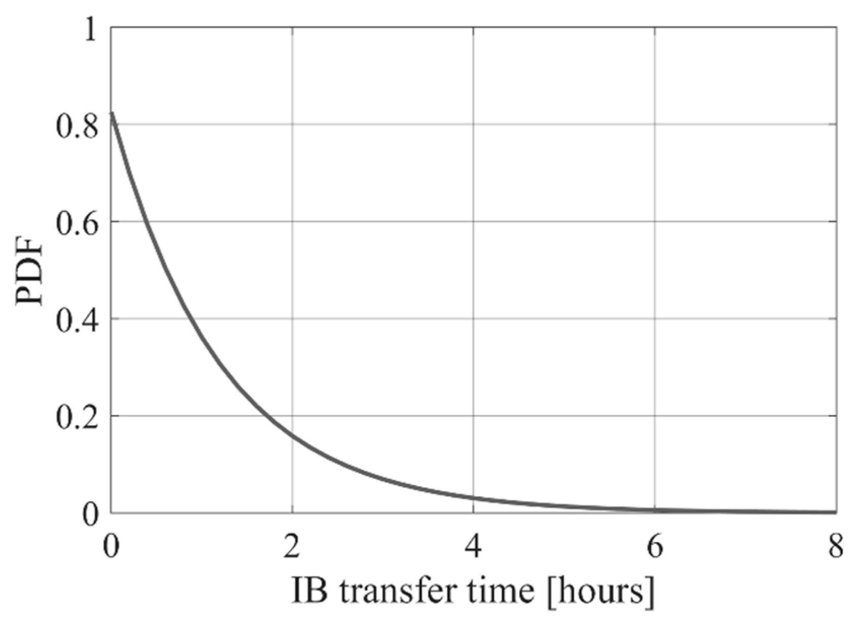
• J—IB transfer and maneuvering time. Although an IB is assumed to remain within its operating area at all times, the exact position from which an IB starts to move towards a ship calling for assistance is not known. Therefore, the related “transfer time” (hours) is determined probabilistically based on an assumed distribution. Once an IB has reached a ship or convoy in need of assistance, before the assistance may start, the IB must maneuver itself into an appropriate position ahead of the ship(s) that are to be assisted. Additionally, in case the ship(s) are stuck in ice, the icebreaker must first cut loose the ship(s) by breaking the surrounding ice. The corresponding maneuvering time is determined probabilistically based on an assumed distribution. The ship entity will remain in the block for a time corresponding to the sum of the determined IB transfer and maneuvering times.
• K—Ship waiting to join a convoy. A ship entity waiting in block K will form a convoy with the first IB-assisted ship entity exiting block J. The IB-assisted ship entity arriving from block J is assumed to have priority access to the IB, meaning that it will be assisted by the IB until it has reached its destination or is deemed able to continue independently (see description of block D—“Need for IB assistance”). The ship entity joining the convoy from block K, on the other hand, will be assisted over one leg only after which it needs to call for further IB assistance if needed.
• L—Speed with IB assistance. The speed (knots) of a ship assisted by an IB is determined as the lower of the achievable speed of the assisted ship and the achievable speed of the assisting IB. In other words, the speed is either limited by the assisted ship or by the IB. The achievable speed of the assisted ship is determined based on ship model-specific hv curves for “Assistance at distance”, examples of which are presented in Figure 3. The achievable speed of the IB is determined as per the description of block C—“Speed without IB assistance”. In the case of convoy operation, as a simplification, the speed of each assisted ship is determined separately as described above.
• M—Leg time with IB assistance. The leg time (hours) for an IB-assisted ship or convoy is determined based on the leg distance and the speed as determined in block L. The ship entity or entities will remain in the block for a time corresponding to the calculated leg time.

The performance of the FSWNS depends on many stochastic factors. In the simulation, as explained above, random variables are generated by drawing random numbers from variable-specific distributions. It can be noted that using MATLAB, the generation of streams of random values is as default repeatable, meaning that separate simulation runs result in identical streams of random values. This is well suited to analyze the influence of variations in single parameter values or distributions. However, in order to analyze how the system performs under different combinations of parameter values, independent sets of random values must be generated.

A general challenge related to the modelling of stochastic factors of the FSWNS is the lack of relevant data. In this study, four stochastic variables are considered: (a) the presence of brash ice channels as determined in block B, (b) the time it takes for an IB to reach a ship in need of assistance as determined in block J, (c) the duration of the IB maneuverings required before an IB assistance can start, and (d) uncertainty in the assumed $H_{eq\_avg}$ and $H_{eq\_max}$ values. Examples of how these variables can be specified are presented in Section 4.

Using DES, the simulated period is divided into equal time steps. In this study, the length of the applied time step is one hour. This means that a change in the state of the system is occurring every hour. Another important time unit is the number of days since the start of the simulation, based on which date is defined. The date is important as it, as explained above, defines the prevailing ice conditions along a specific leg and whether a brash ice channel is present.

As per Figure 1, IBs are assumed to operate within a limited IB operating area. In the simulation, this means that once an IB resource has assisted a ship entity to the border of its operating area, it will leave the ship. If further assistance is needed, a ship entity will request an IB resource from within the IB operating area that it is entering. Thus, in line with the available maritime traffic data, a ship entity might be assisted by several different IB resources on its way towards its destination. In this case, the total waiting time for IB assistance is the accumulated sum of the waiting times related to each instance of IB assistance.

3.3. Generalizations and Assumptions

Resulting from the complexity of the FSWNS, as well as due to various identified knowledge gaps and technical limitations of the applied simulation technique, the simulation model simplifies and generalizes some of the characteristics and mechanisms of the FSWNS. Specifically, the following generalizations and assumptions are noted:

• Concept of equivalent ice thickness. As applied in this approach, the concept of equivalent ice thickness rests on the assumption that an ice cover of a specific equivalent thickness results in the same level of hull resistance as continuous level ice of the same thickness [21]. A weakness of this concept is that it fails to account for individual ice features (e.g., individual ice ridges) that might stop a ship [22]. Anyhow, based on [23], for the simulation of ships operating on the Baltic Sea, the concept appears well suited.
• The use of hv-curves. The use of hv curves to model the speed of ships in ice is well established. It should be noted that this approach typically rests on the assumption that ships operate at a fixed engine load (typically near the maximum continuous rating), which is not always true [24]. However, currently, there is no general and publicly available approach to eliminate this assumption.
• Multi-ship convoy operations. In the simulation, convoy operations in which an IB assists two ships at a time occur whenever two ships need IB assistance over the same distance at the same time. Convoy operations in which three or more ships are assisted at one time are not considered. These simplified assumptions are needed as it is not entirely clear under what conditions convoy operations may occur. The ice resistance of a ship being assisted by an IB tends to increase as a function of the distance between the ship and the assisting IB. Therefore, because a significant safety distance is required between ships operating in a convoy, multi-ship convoy operations require a higher ice-going capability from the involved ships [20]. As a result, considering the EEDI regulations and other measures lowering the average ice-going capability of modern ships, convoy operations and particularly those in which an IB assists more than two ships at a time are expected to remain rare in the future, especially during periods of heavy ice conditions. For this reason, the exclusion of convoy operations involving more than two assisted ships is not expected to significantly reduce the accuracy of the simulation model when applied to simulate heavy ice condition scenarios.
• IB transit times. Due to limitations set by the applied simulation technique, the exact location from which an available IB starts to move towards a ship in need of IB assistance is not known. Therefore, the duration of the IB transit is determined probabilistically based on statistics. In the real world, the master of an IB may try to minimize a ship’s waiting time by predicting where assistance will be needed, and if possible, start to proceed towards that area in advance. Thus, particularly during periods of low demand for IB assistance, the above-described approach is likely conservative. On the other hand, in periods of high demand for IB assistance, IB waiting times appear to be primarily driven by the availability of IBs, meaning that the relationship between transit times and ships’ total IB waiting times is small.
• Criteria for providing of IB assistance. In the simulation, IB assistance is provided if a ship’s independently achievable speed falls below a specific limit value (e.g., 1.5 knots) in the worst assumed ice conditions along a leg. In the real-world, the criteria for IB assistance likely depends on the operating situation so that the criteria are stricter during times of high demand for IB assistance. In addition, the decision on whether IB assistance is to be provided, or requested, is also likely influenced by the individual judgement of the masters of the involved ships. Currently, there are no publicly available models or principles based on which such decision-making could be modelled accurately.
• Active measures by the crew. As per the simulation model structure presented in Figure 1, the network of routes along which ships operate throughout a simulation is assumed fixed. This means that active crew measures, such as maneuverings to avoid local areas with difficult ice conditions, are not considered. As a result, particularly for sea areas with partially ice-covered waters, the simulation outcome can be assumed conservative. In principle, this limitation could be overcome, e.g., by applying a voyage optimization tool as proposed by [25]. However, this would make the approach significantly more complex.

4. Validation

4.1. Approach

Validation of the model is carried out based on real-world maritime traffic data obtained through the research project WINMOS II (Winter Navigation Motorways of the Sea II) [26] covering maritime traffic on the Bothnian Bay in the period 15 January–5 February 2010. The accuracy of the model is assessed by comparing simulated and data-based performance indicators, such as the number of port arrivals, the number of instances of IB assistance, and IB waiting times. To capture the stochastic behavior of the system, a total of 35 individual simulation runs are carried out. All considered maritime traffic data are presented in the Appendix A (see

Table A1. List of ships arriving from Kvarken (Point A as per Figure 4).

Entry Time, Point B (h)	Ship Model	Port 1	Port 2	Port 3	PTT 1 (h)	PTT 2 (h)	PTT 3 (h)
1	I	Raahe			43
1	A	Raahe			51
1	P	Oulu	Kemi		5	4
1	K	Kokkola			14
5	N	Kokkola			48
10	K	Kemi			100
24	N	Tornio			46
27	C	Oulu			14
29	K	Kemi			60
40	K	Raahe			61
40	P	Kemi	Oulu		7	7
48	C	Kemi	Kotka		21
53	K	Tornio			77
57	G	Kokkola	Raahe		26	61
59	I	Kokkola			12
63	K	Kokkola			31
65	G	Raahe			89
66	G	Kokkola			86
69	M	Kokkola			20
72	N	Kokkola			48
74	K	Tornio			21
76	F	Kokkola			73
83	G	Raahe	Tornio		64	19
91	C	Oulu			19
91	G	Tornio	Kotka		25
91	G	Kemi			28
92	G	Kokkola	Kemi		60	53
93	G	Kokkola			31
95	O	Kemi	Oulu		4	12
97	K	Tornio	Kemi		22	36
99	K	Tornio			22
101	C	Kokkola			50
108	K	Raahe			69
111	G	Raahe			51
113	K	Kokkola			43
119	K	Oulu			35
122	K	Oulu			108
125	G	Kokkola	Kemi	Oulu	35	73	65
126	K	Tornio			19
133	G	Tornio			65
134	A	Raahe			162
135	K	Tornio	Raahe		22	30
139	L	Kemi			51
140	C	Oulu			19
144	N	Oulu			34
152	L	Oulu			17
156	P	Oulu	Kemi		6	8
157	G	Kemi			122
157	G	Raahe			68
158	K	Kokkola			27
160	C	Kemi			30
165	G	Raahe	Oulu		51	41
167	N	Oulu			23
172	K	Tornio			41
178	K	Oulu			17
182	F	Kokkola			32
192	N	Raahe			52
200	K	Kokkola			81
200	K	Kokkola			76
206	P	Oulu	Kemi		8	7
207	J	Kokkola			64
207	A	Raahe			57
214	K	Kokkola	Raahe		15	48
220	G	Tornio	Kokkola		50	55
224	M	Raahe			34
228	F	Kokkola			18
228	K	Kokkola			97
228	C	Oulu			-3
228	C	Raahe	Pori		43
230	G	Tornio			66
235	C	Oulu			6
235	C	Kokkola			7
242	N	Oulu	Tornio		78	21
243	I	Raahe			27
244	G	Tornio	Raahe		20	49
249	K	Tornio	Kemi		28	40
250	K	Oulu			73
260	B	Kokkola			54
261	L	Kokkola			18
262	O	Kemi	Oulu		7	7
263	K	Tornio	Kotka		45
266	P	Kemi			116
268	M	Raahe			69
275	G	Kokkola			64
278	K	Tornio	Raahe		44	88
293	G	Tornio			65
298	C	Kokkola			24
310	L	Oulu			18
311	K	Oulu	Kemi		31	68
319	K	Raahe			54
321	K	Oulu	Pori		70
323	P	Oulu	Kemi		10	11
332	K	Kokkola			71
336	A	Raahe			47
337	B	Kokkola			24
339	I	Kemi			17
352	G	Kokkola			111
360	N	Oulu			34
364	K	Kokkola			21
370	P	Kemi	Oulu		7	8
374	M	Kokkola			22
383	C	Kokkola			7
384	N	Tornio			46
393	N	Oulu	Tornio		104	23
394	F	Raahe	Kokkola		41	65
401	K	Tornio
407	G	Kemi	Raahe		32	4
419	E	Oulu			14
419	A	Raahe			40
424	G	Kokkola			94
425	G	Tornio	Raahe		32	47
426	P	Oulu			6
434	B	Tornio	Raahe	Pori	147	29
448	G	Tornio			79
455	K	Kokkola			29
457	A	Raahe			37
470	J	Kokkola			64
473	K	Kemi	Oulu		82	50
474	K	Raahe			64
481	K	Raahe			73
486	B	Kokkola			17
486	K	Tornio			29
490	G	Kemi			39
493	G	Oulu			84
496	K	Oulu			15
496	G	Tornio			77
504	N	Raahe			52
514	B	Kokkola			239
514	P	Oulu	Kemi		9	7
519	H	Kemi			145
531	K	Raahe	Tornio		18	79
536	P	Kemi	Oulu		8	10
542	C	Oulu			22
543	K	Raahe	Tornio		45	23
554	G	Raahe	Oulu		25	58
562	K	Raahe	Kokkola
563	K	Tornio			47
563	K	Raahe			8
567	N	Oulu	Tornio		101	45
574	K	Raahe			68
576	G	Oulu			74
576	N	Oulu			34
577	G	Kemi	Tornio		44	23
584	G	Tornio			67
588	K	Kokkola			19
593	L	Oulu			21
593	K	Kemi	Oulu		52	45
595	O	Kemi	Oulu		9	7
596	H	Oulu
610	I	Raahe			14
621	A	Raahe			15
626	C	Kokkola			49
629	L	Kemi			17
630	G	Tornio			65
636	K	Tornio	Raahe		30	77
648	N	Tornio			46
659	G	Raahe			17
660	M	Kokkola			28
670	K	Tornio	Kokkola
679	G	Kemi			51
681	K	Kemi	Kokkola
682	P	Oulu	Kemi		8	6
683	L	Kokkola			15
701	C	Kemi			15
708	P	Kemi	Oulu		8	8
710	F	Kokkola			64
718	D	Raahe			92
725	K	Raahe			7
736	L	Oulu			29
744	N	Oulu			34
753	N	Oulu	Tornio
754	K	Tornio			39
755	F	Raahe	Kokkola		14	45
764	G	Kokkola			32
765	O	Kemi	Oulu

and

Table A2. List of ships arriving from northern Sweden (Point B as per Figure 4).

Entry Time, Point B (h)	Ship Model	Port 1	Port 2	Port 3	PTT 1 (h)	PTT 2 (h)	PTT 3 (h)
31	A	Raahe			39
67	A	Raahe			15
110	A	Raahe			29
137	A	Raahe			33
155	M	Raahe			18
164	A	Raahe			49
249	A	Raahe			21
371	A	Raahe			48
388	M	Raahe			12
455	A	Raahe			49
455	M	Raahe			11
541	A	Raahe			18
593	A	Raahe			18
608	A	Raahe			40
645	A	Raahe			43
686	A	Raahe			74
737	M	Raahe			40
758	A	Raahe			52

).

4.2. Simulation Input

4.2.1. Maritime Traffic

Information on ships entering the Bothnian Bay is specified based on the above-mentioned maritime traffic data, an extract of which is presented in

Table 1. Extract of maritime traffic data. The port turnaround time (PTT) represents the total duration of a port visit including port maneuvering time, mooring time, and cargo handling time.

Entry Time, Point A (h)	Ship Model	Port 1	Port 2	Port 3	PTT 1 (h)	PTT 2 (h)	PTT 3 (h)
76	F	Kokkola			73
83	G	Raahe	Tornio		64	19
91	C	Oulu			19
91	G	Tornio	Kotka		25
91	G	Kemi			28
92	G	Kokkola	Kemi		60	53

. The entry time is specified in hours from the start of the simulation at midnight 15 January 2010. As per Figure 4, ships arriving from the South (Kvarken) are assumed to enter the considered area at point A, whereas ships arriving from the Northwest (northern Sweden, Lulea) are assumed to enter at point B. Entered ships visit 1–3 ports before they leave the system. The total duration of each port visit is determined in terms of the port turnaround time (PTT) as specified by the maritime traffic data.

4.2.2. Ship Performance Data

The considered maritime traffic data covers ships representing some 16 different models. For each ship model, as per Figure 5, the achievable speed in ice is determined in terms of ship model-specific hv curves representing three different modes of operation: (a) IB assistance at distance, (b) operation in a brash ice channel, and (c) independent operation in level ice. All hv curves were determined within the research project WINMOS II [26] based on ice resistance formulas and design particulars of the corresponding real-world ships.

4.2.3. Ice Conditions

Based on ice charts provided by [27], for each considered date and navigation leg, the prevailing ice conditions are determined in terms of the average ice conditions $H_{eq\_avg}$ and the most difficult ice conditions $H_{eq\_max}$. Specifically, the average ice conditions along a leg $H_{eq\_avg}$ is determined as per Equation (2).

$$H_{eq\_avg}=\frac{H_{min}+H_{max}}{2}\ast \frac{C_{min}+C_{max}}{2}+H_{ridging\_avg},$$

(2)

where $H_{min}$ represents the minimum ice thickness, $H_{max}$ represents the maximum ice thickness, $C_{min}$ represents the minimum ice concentration, $C_{max}$ represents the maximum ice concentration, and $H_{ridging\_avg}$ is an assumed 6 cm increase in equivalent ice thickness caused by ridges (where ice ridging occurs). The assumed value of $H_{ridging\_avg}$ is based on [28], according to which ice ridges in the Bothnian Bay increase the level ice thickness by 6–14 cm equivalent ice thickness. The most difficult ice conditions occurring along a leg $H_{eq\_max}$ is determined as per Equation (3).

$$H_{eq\_max}=H_{max}\ast C_{max}+H_{ridging\_max},$$

(3)

where $H_{max}$ represents the maximum ice thickness, $C_{max}$ represents the maximum ice concentration, and $H_{ridging\_max}$ is an assumed 14 cm increase in level ice thickness caused by ridges (where ice ridging occurs) [28].

Extracts of calculated and applied $H_{eq\_avg}$ and $H_{eq\_max}$ values are presented in

Table 2. Extract of $H_{eq\_avg}$ (cm) values.

Date	L1	L2	L3	L4	L5	L6	L7	L8	L9	L10	L11	L12	L13	L14	L15
2 February 2010	4	5	5	33	5	5	5	38	21	32	38	21	38	38	43
3 February 2010	4	5	5	33	5	5	5	38	21	32	38	21	38	38	43
4 February 2010	4	5	5	33	5	5	5	38	21	32	38	21	38	38	43
5 February 2010	23	23	23	40	23	23	23	38	23	38	38	39	45	45	45
6 February 2010	23	23	23	40	23	23	23	38	23	38	38	39	45	45	45
7 February 2010	23	23	23	40	23	23	23	38	23	38	38	39	45	45	45

and

Table 3. Extract of $H_{eq\_max}$ values (cm).

Date	L1	L2	L3	L4	L5	L6	L7	L8	L9	L10	L11	L12	L13	L14	L15
2 February 2010	5	5	5	40	5	5	5	50	30	30	50	30	50	50	54
3 February 2010	5	5	5	40	5	5	5	50	30	30	50	30	50	50	54
4 February 2010	5	5	5	40	5	5	5	50	30	30	50	30	50	50	54
5 February 2010	36	36	36	50	36	36	36	50	36	50	50	50	60	60	59
6 February 2010	36	36	36	50	36	36	36	50	36	50	50	50	60	60	59
7 February 2010	36	36	36	50	36	36	36	50	36	50	50	50	60	60	59

. The complete ice data are found in Appendix B (see

Table A3. $H_{eq\_avg}$ (cm) determined by date and leg (L).

Date	L1	L2	L3	L4	L5	L6	L7	L8	L9	L10	L11	L12	L13	L14	L15
15 January 2010	6	14	32	13	29	24	32	30	23	32	30	20	33	33	25
16 January 2010	6	14	32	13	29	24	32	30	23	32	30	20	33	33	25
17 January 2010	6	14	32	13	29	24	32	30	23	32	30	20	33	33	25
18 January 2010	6	14	32	13	29	24	32	30	23	32	30	20	33	33	25
19 January 2010	6	14	32	13	29	24	32	30	23	32	30	20	33	33	25
20 January 2010	6	14	32	13	29	24	32	30	23	32	30	20	33	33	25
21 January 2010	6	14	32	13	29	24	32	30	23	32	30	20	33	33	25
22 January 2010	8	9	10	33	9	9	10	30	23	32	30	20	33	33	32
23 January 2010	8	9	10	33	9	9	10	30	23	32	30	20	33	33	32
24 January 2010	8	9	10	33	9	9	10	30	23	32	30	20	33	33	32
25 January 2010	8	9	10	33	9	9	10	30	23	32	30	20	33	33	32
26 January 2010	8	9	10	33	9	9	10	30	23	32	30	20	33	33	32
27 January 2010	8	9	10	33	9	9	10	30	23	32	30	20	33	33	32
28 January 2010	8	9	10	33	9	9	10	30	23	32	30	20	33	33	32
29 January 2010	4	5	5	33	5	5	5	38	21	32	38	21	38	38	43
30 January 2010	4	5	5	33	5	5	5	38	21	32	38	21	38	38	43
31 January 2010	4	5	5	33	5	5	5	38	21	32	38	21	38	38	43
1 February 2010	4	5	5	33	5	5	5	38	21	32	38	21	38	38	43
2 February 2010	4	5	5	33	5	5	5	38	21	32	38	21	38	38	43
3 February 2010	4	5	5	33	5	5	5	38	21	32	38	21	38	38	43
4 February 2010	4	5	5	33	5	5	5	38	21	32	38	21	38	38	43
5 February 2010	23	23	23	40	23	23	23	38	23	38	38	39	45	45	45
6 February 2010	23	23	23	40	23	23	23	38	23	38	38	39	45	45	45
7 February 2010	23	23	23	40	23	23	23	38	23	38	38	39	45	45	45
8 February 2010	23	23	23	40	23	23	23	38	23	38	38	39	45	45	45
9 February 2010	23	23	23	40	23	23	23	38	23	38	38	39	45	45	45
10 February 2010	23	23	23	40	23	23	23	38	23	38	38	39	45	45	45
11 February 2010	23	23	23	40	23	23	23	38	23	38	38	39	45	45	45
12 February 2010	41	33	33	40	33	33	33	45	33	45	45	39	55	55	52
13 February 2010	41	33	33	40	33	33	33	45	33	45	45	39	55	55	52
14 February 2010	41	33	33	40	33	33	33	45	33	45	45	39	55	55	52
15 February 2010	41	33	33	40	33	33	33	45	33	45	45	39	55	55	52

and

Table A4. $H_{eq\_max}$ (cm) determined by date and leg (L).

Date	L1	L2	L3	L4	L5	L6	L7	L8	L9	L10	L11	L12	L13	L14	L15
15 January 2010	20	20	45	20	30	36	36	40	30	30	40	30	40	40	39
16 January 2010	20	20	45	20	30	36	36	40	30	30	40	30	40	40	39
17 January 2010	20	20	45	20	30	36	36	40	30	30	40	30	40	40	39
18 January 2010	20	20	45	20	30	36	36	40	30	30	40	30	40	40	39
19 January 2010	20	20	45	20	30	36	36	40	30	30	40	30	40	40	39
20 January 2010	20	20	45	20	30	36	36	40	30	30	40	30	40	40	39
21 January 2010	20	20	45	20	30	36	36	40	30	30	40	30	40	40	39
22 January 2010	15	15	15	40	15	15	15	40	44	32	40	44	40	40	44
23 January 2010	15	15	15	40	15	15	15	40	44	32	40	44	40	40	44
24 January 2010	15	15	15	40	15	15	15	40	44	32	40	44	40	40	44
25 January 2010	15	15	15	40	15	15	15	40	44	32	40	44	40	40	44
26 January 2010	15	15	15	40	15	15	15	40	44	32	40	44	40	40	44
27 January 2010	15	15	15	40	15	15	15	40	44	32	40	44	40	40	44
28 January 2010	15	15	15	40	15	15	15	40	44	32	40	44	40	40	44
29 January 2010	5	5	5	40	5	5	5	50	30	30	50	30	50	50	54
30 January 2010	5	5	5	40	5	5	5	50	30	30	50	30	50	50	54
31 January 2010	5	5	5	40	5	5	5	50	30	30	50	30	50	50	54
1 February 2010	5	5	5	40	5	5	5	50	30	30	50	30	50	50	54
2 February 2010	5	5	5	40	5	5	5	50	30	30	50	30	50	50	54
3 February 2010	5	5	5	40	5	5	5	50	30	30	50	30	50	50	54
4 February 2010	5	5	5	40	5	5	5	50	30	30	50	30	50	50	54
5 February 2010	36	36	36	50	36	36	36	50	36	50	50	50	60	60	59
6 February 2010	36	36	36	50	36	36	36	50	36	50	50	50	60	60	59
7 February 2010	36	36	36	50	36	36	36	50	36	50	50	50	60	60	59
8 February 2010	36	36	36	50	36	36	36	50	36	50	50	50	60	60	59
9 February 2010	36	36	36	50	36	36	36	50	36	50	50	50	60	60	59
10 February 2010	36	36	36	50	36	36	36	50	36	50	50	50	60	60	59
11 February 2010	36	36	36	50	36	36	36	50	36	50	50	50	60	60	59
12 February 2010	54	46	46	50	46	46	46	60	46	59	60	59	70	70	64
13 February 2010	54	46	46	50	46	46	46	60	46	59	60	59	70	70	64
14 February 2010	54	46	46	50	46	46	46	60	46	59	60	59	70	70	64
15 February 2010	54	46	46	50	46	46	46	60	46	59	60	59	70	70	64

). It should be noted that the assumed values of $H_{eq\_avg}$ and $H_{eq\_max}$ are subject to significant uncertainty originating both from the source, i.e., the ice charts, which presents ice data in terms of approximate thickness and concentration ranges, and from the assumption that the ice conditions are homogenous over the considered navigation legs. To account for this uncertainty, during an individual simulation run, each value of $H_{eq\_avg}$ and $H_{eq\_max}$ presented in Table 2 and Table 3 is multiplied with two coefficients, one representing the uncertainty in ice thickness, and the other representing the uncertainty in ice concentration. Both coefficients are determined by drawing a random number from a normally distributed set with a mean of 1 and a standard deviation of 10%.

Ships operating in ice may encounter brash ice channels created and maintained by IBs and other ships. The duration for which an ice channel remains open and navigable depends on multiple factors including the amount of maritime traffic, the local geography, as well as the prevailing wind and currents [29]. In addition, strong winds in combination with a physical boundary might result in compressive ice, which may significantly increase a ship’s ice resistance [30]. Anyhow, due to a lack of related data and suitable engineering models, such factors are not systematically considered. Instead, it is assumed that along fairways with very significant traffic (L 1 and 2), a brash ice channel is available with a 75% probability, along fairways with significant traffic (L 3, 5, 6, 7, 9, 10, and 12), a brash ice channel is available with a 50% probability. On the open sea, where the traffic is limited (L 15), brash ice channels are assumed not to be present. In protected waters with fast ice (L 4, 8, and 11, 13, and 14), brash ice channels are assumed to be present throughout the simulation.

4.2.4. IB Transfer and Maneuvering Times

Due to a lack of available real-world data, the time it takes for an available IB to reach a ship in need of assistance, in the following referred to as IB transfer time, is determined based on statistics of simulated transfer times obtained from research project WINMOS II [26], generated based on the mathematical simulation approach by [12]. Following the obtained data, IB transfer times are assumed to be exponentially distributed as per the probability density function (PDF) in Figure 6. Accordingly, the time it takes for an available IB to reach a ship in need of assistance is assumed to be in the range of 0–8 h. The maximum transfer time may correspond to a situation where an IB must cover some 80 NM at an average speed of 10 knots to reach a ship in need of assistance. This distance is roughly equivalent to, for instance, the distance L1–L4 (see Figure 4). The IB maneuvering time is assumed to follow a normal distribution with a mean value of 20 min and a standard deviation of 5 min.

4.2.5. IB Assistance Parameters

During the considered period 15 January–15 February 2010, as per ice charts issued by [27], IB assistance in the Bothnian Bay is provided by four IBs: Fennica, Urho, Otso, and Kontio. However, as a simplification, all icebreakers are assumed to have an ice-going capability corresponding to that of Otso. The IBs are assumed to operate within their operating area as defined by Figure 1. IB assistance is provided to those ships whose independently achievable speed is estimated to fall below 1.5 knots in the worst ice conditions ($H_{eq\_max}$) along a leg. IB assistance is continued until a ship has been assisted to a waypoint from which it can continue independently at a minimum speed of 8 knots. During icebreaker assistance, the maximum speed of the IB and the assisted ship(s) is assumed limited to 12 knots.

4.3. Validation Results

4.3.1. Real World vs. Simulated Number of Port Visits

Figure 7a presents the real-world number of ship arrivals per destination port, the corresponding simulated values for 35 individual simulation runs, and the mean of the simulated values. As per the figure, the simulated values agree well with the data. This indicates that the traffic flows within the simulation model follow the data and that the simulated ship transit times are in the same range as, or lower than, the real-world transit times.

4.3.2. Real World vs. Simulated Number of Assisted Voyages

Figure 7b presents the real-world number of instances of IB assistance per destination port, the corresponding simulated values for 35 individual simulation runs, and the mean of the simulated values. The presented numbers include all instances of IB assistance received by ships on their way to or from individual ports. As ships are often assisted at multiple times during a single voyage, the number of instances of assistance is higher than the number of ships that received assistance. As shown by the figure, for all ports the mean values of the simulations agree quite well with the data. However, the variation between individual simulation runs is significant. The standard deviation between the mean values and the data is 13%. As per the data, the total number of instances of assistance is 192 whereas the corresponding simulated mean value is 213 (+11%).

4.3.3. Real World vs. Simulated IB Waiting Times

Figure 7c presents the real-world mean IB waiting time per destination port, the corresponding simulated values for 35 individual simulation runs, and the mean of the simulated values. The presented values correspond to the mean waiting time for all instances of IB assistance related to a ship heading to or leaving from a given port. As shown by the figure, in general the data and the mean of the simulated values agree quite well. The deviation is the largest in the case of the port of Kokkola. This is because most ships use the fairway outside Kokkola (Leg 1–2), which in the simulation apparently occasionally results in bottleneck situations. In the real world, such bottleneck situations might be avoided by various factors not considered in the applied simulation model (e.g., in the real world an IB might perhaps if needed assist more than two ships at a time, or the likelihood of an ice channel being present might be higher than assumed during periods of heavy traffic). As for the instances of assistance, the variation between individual simulation runs is significant. The overall standard deviation between the mean values of the individual simulation runs and the data is 18%. As per the data, the mean IB waiting time is 3.0 h, whereas the corresponding simulated number is 3.2 h (+7%).

4.3.4. Confidence Intervals

The statistical agreement between the maritime data and the simulation outcome is tested in terms of confidence intervals. Specifically, for each of the simulated port-specific number of instances of IB assistance and mean IB waiting times, we consider an approximate 95 confidence interval determined by multiplying the standard deviation (${\sigma }_{sim}$) of the mean values (${\mu }_{sim}$) of 35 independent simulation runs by 2. As per

Table 4. Approximated 95% confidence interval for the simulated port-specific number of instances of IB assistance.

Port	Maritime Data	${\mathit{\mu }}_{\mathit{s}\mathit{i}\mathit{m}}$	${\mathit{\sigma }}_{\mathit{s}\mathit{i}\mathit{m}}$	${\mathit{\mu }}_{\mathit{s}\mathit{i}\mathit{m}}-2{\mathit{\sigma }}_{\mathit{s}\mathit{i}\mathit{m}}$	${\mathit{\mu }}_{\mathit{s}\mathit{i}\mathit{m}}+2{\mathit{\sigma }}_{\mathit{s}\mathit{i}\mathit{m}}$
Kokkola	18	28.7	6.5	15.8	41.7
Raahe	48	38.7	5.5	27.6	49.7
Oulu	50	52.5	6.8	38.8	66.1
Kemi	28	38.4	5.2	28.0	48.9
Tornio	48	54.5	7.1	40.3	68.6

and

Table 5. Approximated 95% confidence interval for the simulated port-specific mean IB waiting times (hours).

Port	Maritime Data	${\mathit{\mu }}_{\mathit{s}\mathit{i}\mathit{m}}$	${\mathit{\sigma }}_{\mathit{s}\mathit{i}\mathit{m}}$	${\mathit{\mu }}_{\mathit{s}\mathit{i}\mathit{m}}-2{\mathit{\sigma }}_{\mathit{s}\mathit{i}\mathit{m}}$	${\mathit{\mu }}_{\mathit{s}\mathit{i}\mathit{m}}+2{\mathit{\sigma }}_{\mathit{s}\mathit{i}\mathit{m}}$
Kokkola	1.7	3.6	1.4	0.7	6.4
Raahe	3.5	3.5	1.2	1.0	6.0
Oulu	3.8	3.0	1.6	−0.2	6.1
Kemi	2.3	3.1	1.0	1.1	5.1
Tornio	3.8	2.9	0.9	1.2	4.7

, for each of the simulated performance metrics, the maritime data fall within the obtained 95% confidence interval.

4.3.5. Sensitivity Analysis

Due to the high degree of complexity and randomness of the FSWNS, and the general lack of related data, the present simulation model rests on several assumptions. These concern the prevailing ice conditions, the IB transfer times, and the presence of pre-existing ice channels, among others. To assess the sensitivity of the simulation outcome to those assumptions, a sensitivity analysis is carried out. As per Figure 8, the sensitivity analysis indicates that the simulated number of instances of IB assistances is sensitive to variations in the assumed $H_{eq}$-values, but especially to assumptions concerning the presence of pre-existing ice channels. Specifically, by increasing or decreasing the assumed $H_{eq}$-values by 20%, the instances of assistance increase by 13% or decrease by 30%, respectively. By assuming that all those brash ice channels that as default are assumed to be present with a 50% probability (see Section 4.2.3) are present at all times, the instances of assistance decrease by 98%, whereas by assuming that the same ice channels are absent at all times, the instances of assistances increase by 45%.

The sensitivity analysis further indicates that the mean IB waiting time is sensitive to all the analyzed assumption variations. Specifically, by increasing or decreasing the assumed $H_{eq}$-values by 20%, the simulated mean waiting time for IB assistance increases by 6% or decreases by 23%, respectively. By increasing or decreasing the assumed IB transfer times by 50%, the simulated mean waiting time for IB assistance increases by 9% or decreases by 47%, respectively. By assuming that all those brash ice channels that as default are assumed to be present with a 50% probability (see Section 4.2.3) are present at all times, the mean waiting time decreases by 86%, whereas by assuming that the same ice channels are absent at all times, the waiting time increases by 69%.

4.3.6. Validation Summary

The above validation indicates that the proposed simulation approach works in principle. Regarding the number of ship arrivals per port, the simulation agrees well with the data. Regarding the number of instances of IB assistance and IB waiting times, the overall standard deviations between the averages of 35 independent simulation runs and the data are 13% and 18%, respectively. For each of the simulated metrics, the data fall within an approximated 95% confidence interval.

On average, the simulation appears to somewhat overestimate both the number of instances of assistance (+11%) and the IB waiting times (+7%). The overestimated number of assistances may indicate that, in the real world, ships are occasionally assisted over larger distances than the fixed IB operating areas assumed in the simulation. The overestimated mean IB waiting time, in turn, may in part be explained by the large individual peak values observed in Figure 7c. In the real world, such peak values can perhaps be avoided by factors not considered in the present simulation model, such as convoy operations including more than two ships and various active measures by the masters of the involved ships.

It should also be noted that the available maritime data, or the interpretation thereof, may include some errors. For instance, in individual cases, it is reported that a ship has received multiple instances of IB assistance during its inward voyage, but none during its outward voyage even though both voyages would have occurred in similar ice conditions. In addition, occasionally it appears like the data, instead of including all instances of IB assistance received by a ship on its way to or from a port, only include the last or the first instance of IB assistance before port arrival or after departure. Further studies are needed to identify and address such possible inconsistencies.

5. Case Study: Impact of the EEDI on the Operating Performance of the FSWNS

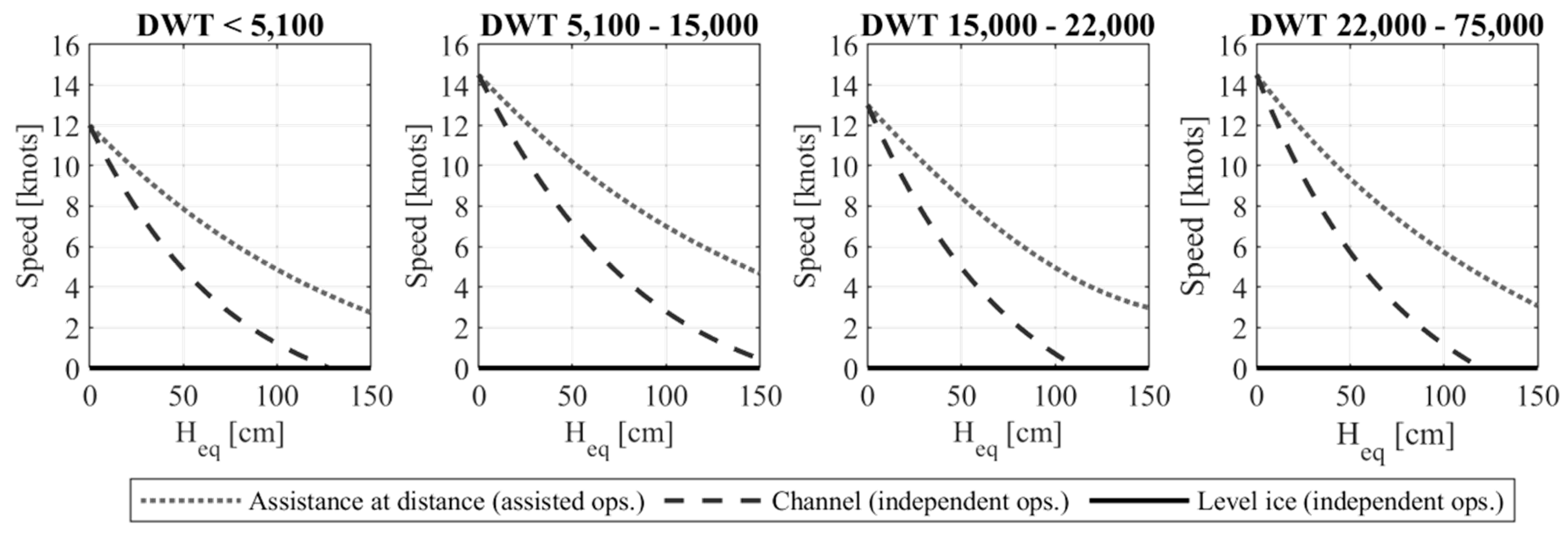
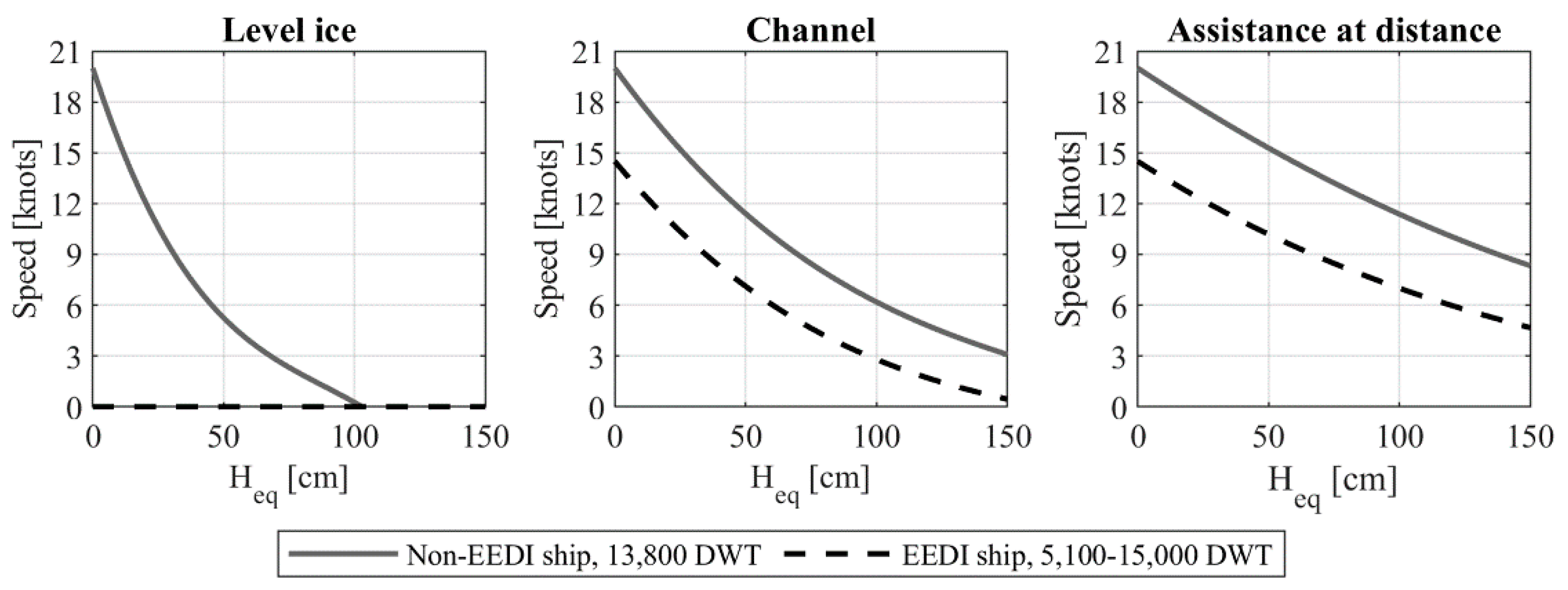
As the EEDI is enforced on new ships only, the existing fleet of ships will only gradually be replaced by EEDI compliant ships. This case study is carried out for scenarios where either one-third (33%) or two-thirds (66%) of arriving ships, randomly selected, have been replaced by new EEDI compliant ships. It is further assumed that the achievable speed in ice of the new EEDI compliant ships is dependent on their size in DWT as per Figure 9. Accordingly, it is assumed that EEDI compliant ships are not able to operate independently in unbroken level ice. Additionally, as per the example presented in Figure 10, it is assumed that the speed of an EEDI compliant ship, when operating in a brash ice channel or with IB assistance, might be significantly lower than that of a corresponding non-EEDI ship. In the case studies, around 30% of the replaced vessels were in the category DWT < 5100, around 60% were in the category DWT 5100–15,000, and around 10% were in the category DWT 15,000–22,000.

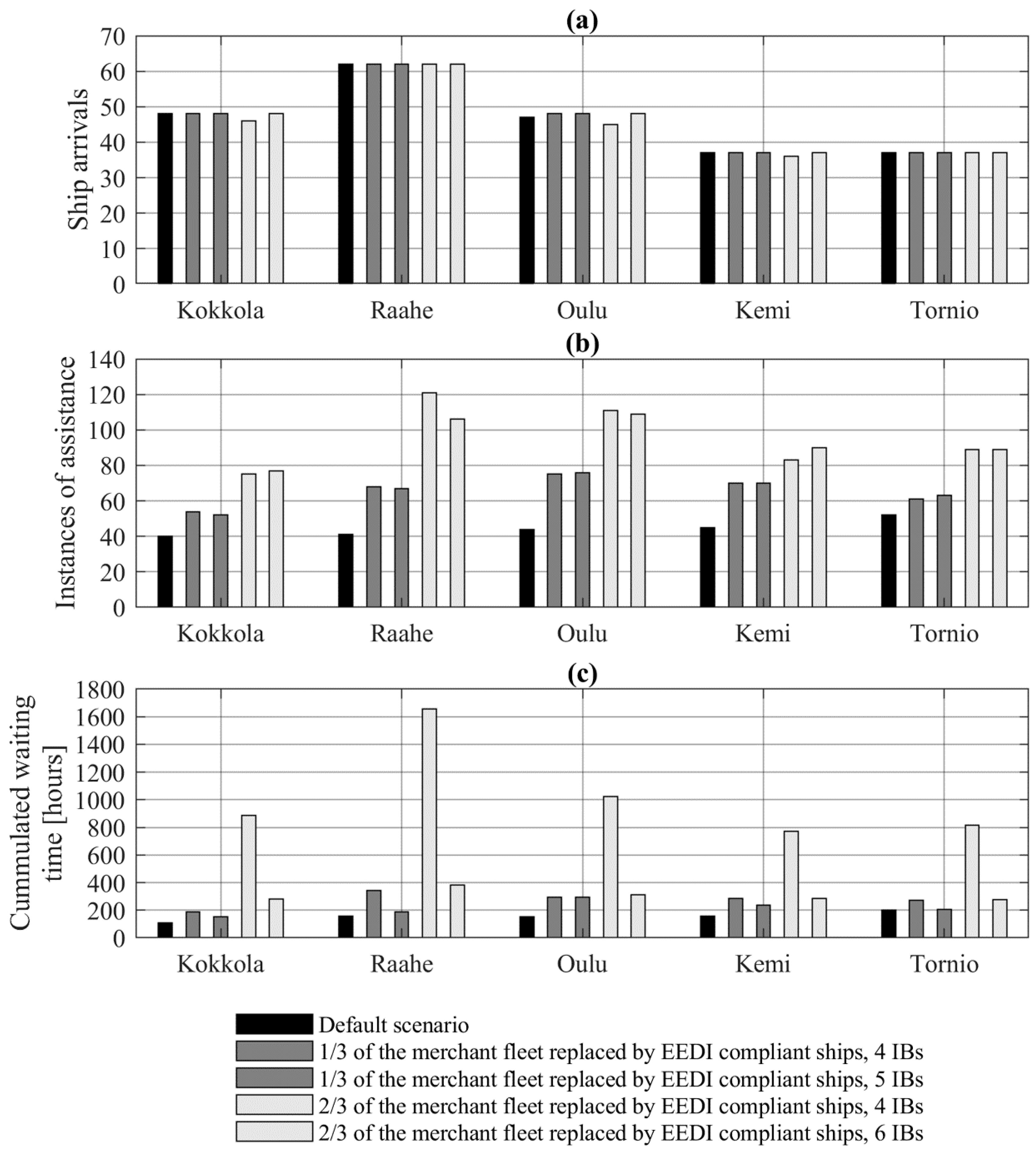
The outcome of the simulated EEDI scenarios is presented in Figure 11. In the first scenario, in which one-third of the current fleet is replaced by EEDI-compliant ships, the number of cases of IB assistance is increased from 222 to 328 (+48%) and the total cumulated waiting times for IB assistance is increased from 775 h to 1378 h (+78%). In the second scenario, in which two-thirds of the current fleet is replaced with EEDI-compliant ships, the total number of cases of IB assistance is increased from 222 to 479 (+116%) and the total cumulated waiting times for IB assistance is increased from 775 h to 5157 h (+565%). In the second scenario, due to the extended waiting times for IB assistance, the total number of port arrivals decreases from 231 to 226 (−2%).

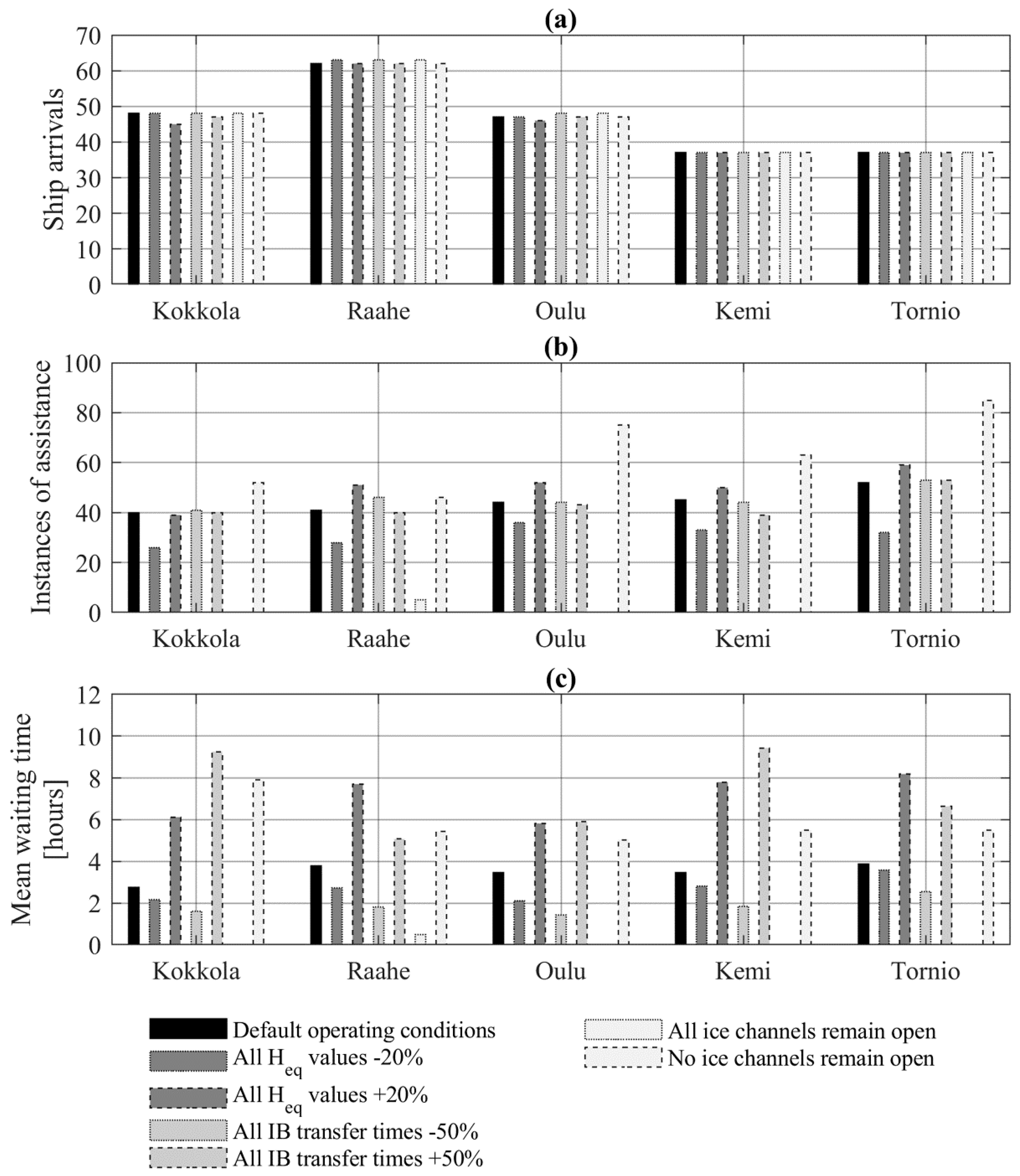
Additional simulations were carried out to assess whether the increase in IB waiting time from the assumed EEDI scenarios could be mitigated by increasing the number of IBs. As per Figure 11, the outcome from the simulations indicates that in the first and second EEDI scenarios, a significant increase in the cumulated IB waiting times can be mitigated by increasing the number of IBs from 4 to 5 and from 4 to 6, respectively. Notwithstanding, due to a lack of relevant data, this assessment is based on generalizing and conservative assumptions concerning the influence of the EEDI on the ice-going capability and other technical characteristics of the merchant fleet. Thus, this case study serves mainly as an example of how the presented approach can be applied to assess the performance of the FSWNS under various operating scenarios.

6. Discussion and Conclusions

This article presents a DES-based approach to predict the operating performance of the FSWNS under different operating scenarios. The approach is validated against real-world data on maritime traffic in the Bothnian Bay in the period 15 January–15 February 2010. In terms of the number of ship arrivals per port, representing the transport capacity of the FSWNS, the simulation agrees well with the data. In terms of the number of instances of IB assistance and IB waiting times, the standard deviations between the averages of 35 independent simulation runs and the data are 13% and 18%, respectively. For each of the simulated metrics, the data fall within an approximated 95% confidence interval. These findings indicate that the proposed DES-based approach can capture the complex behavior of the FSWNS and roughly estimate its operating performance.

Due to various identified knowledge and data gaps, as well as due to technical limitations of the applied simulation approach, the simulation model is based on generalized assumptions concerning convoy operations (a maximum of two ships are assisted by an IB at a time), IB transfer times (probabilistically determined), criteria for providing IB assistance (generalized criteria), and assumptions concerning the presence of brash ice channels (generalized assumptions), among others. A sensitivity analysis indicates that the simulated number of instances of IB assistance and IB waiting times are particularly sensitive to assumptions concerning the presence of brash ice channels. Future research is needed to address the limitations.

Considering the present limitations, the proposed approach appears best suited for scenario-based assessments in which the performance of the FSWNS is assessed for a limited period (e.g., one month) with heavy ice conditions during which the main shipping routes can be assumed fixed. The outcome of such a scenario-based assessment may indicate whether the capacity of the FSWNS under the simulated conditions is sufficient to keep the system in “balance”.

Case studies were carried out in which the approach was applied to assess the impact of replacing various percentages of the present fleet of merchant ships entering the Bay of Bothnia by EEDI-compliant ships. In a scenario in which around one-third of the current fleet is replaced by EEDI-compliant ships, the simulation outcome indicates that the number of cases of IB assistance is increased from 222 to 328 (+48%) and that the cumulated waiting times for IB assistance is increased from 775 h to 1378 h (+78%). In another scenario in which around two-thirds of the current fleet is replaced with EEDI-compliant ships, the simulation outcome indicates that the total number of cases of IB assistance is increased from 222 to 497 (+116%) and that the cumulated waiting times for IB assistance is increased from 775 h to 5157 h (+565%). For the considered scenarios, simulation outcomes indicate that the predicted increase in IB waiting times can be largely mitigated if the number of IBs operating in the area is increased from 4 to 5 or from 4 to 6, respectively. However, due to a lack of detailed data on, e.g., how the EEDI would influence the ice-going capability and other technical characteristics of the affected merchant fleet, the outcome of the analysis is not conclusive.

In summary, the presented approach, which is one of the first attempts to simulate the FSWNS, may provide new insights into the behavior and performance of the FSWNS under different operating scenarios, considering a multitude of interlinked and self-reinforcing system behaviors. As such, the method may be used to support decision-making concerning the management of the FSWNS to meet future goals concerning operational efficiency. In the future, a potential further developed version of the model could be used for more holistic analyses, e.g., to analyze the cost- and energy-efficiency of the FSWNS, considering e.g., the impacts of climate change on sea ice conditions.

References

1. Finnish Shipowners Association. Key Figures of Maritime Transport in Finland. 2020. Available online: https://shipowners.fi/en/competitiveness/key-figures-of-maritime-in-finland/ (accessed on 15 April 2020).
2. Meriliitto. Finland is an Island. 2020. Available online: http://www.meriliitto.fi/?page_id=177 (accessed on 15 April 2020).
3. Finnish Transport and Communications Agency. Statistics on International Shipping; Finnish Transport and Communications Agency Traficom: Helsinki, Finland, 2018. [Google Scholar]
4. FMI. Ice Winter in the Baltic Sea. 2019. Available online: https://en.ilmatieteenlaitos.fi/ice-winter-in-the-baltic-sea (accessed on 15 September 2019).
5. Finnish Transport and Communications Agency. Ice Class Regulations and the Application Thereof; Finnish Transport and Communications Agency: Helsinki, Finland, 2017; Available online: https://www.finlex.fi/data/normit/43682/TRAFI_494_131_03_04_01_00_2016_EN_Jaaluokkamaarays_2017.pdf (accessed on 10 March 2020).
6. Jalonen, R.; Riska, K.; Hänninen, S. Research Report No 57: A preliminary Risk Analysis of Winter Navigation in the Baltic Sea; Winter Navigation Reseach Board/Helsinki University of Technology: Espoo, Finland, 2005. [Google Scholar]
7. ARCTIA. Homepage of Arctia Ltd. 2019. Available online: http://arctia.fi/en/ (accessed on 10 November 2019).
8. SJÖFARTSVERKET. Homepage of the Swedish Maritime Administration. 2019. Available online: https://www.sjofartsverket.se/en/Maritime-services/Winter-Navigation/Our-Icebreakers/ (accessed on 10 November 2019).
9. IMO. Energy Efficiency Measures. International Maritime Organization. Available online: http://www.imo.org/en/OurWork/Environment/PollutionPrevention/AirPollution/Pages/Technical-and-Operational-Measures.aspx (accessed on 10 June 2019).
10. Bergström, M.; Erikstad, S.O.; Ehlers, S. A simulation-based probabilistic design method for arctic sea transport systems. J. Mar. Sci. Appl. 2016, 15, 349–369. [Google Scholar]
11. Craig, D. Discrete-Event Simulation. Memorial University of Newfoundland: St. John’s, NL, Canada, 1996. [Google Scholar]
12. Lindeberg, M.; Kujala, P.; Sormunen, O.-V.E.; Karjalainen, M.; Toivola, J. Simulation model of the Finnish winter navigation system. In Proceedings of the 13th International Marine Design Conference (IMDC 2018), Helsinki, Finland, 10–14 June 2018. [Google Scholar]
13. Finnish Transport and Communications Agency. Ice Classes of Ships; Finnish Transport and Communications Agency: Helsinki, Finland, 2019. [Google Scholar]
14. Baltic Icebreaking Management. Baltic Sea Icebreaking Report 2014–2015; Baltic Icebreaking Management: Helsinki, Finland, 2015. [Google Scholar]
15. International Maritime Organization. 2018 Guidelines on the Method of Calculation of the Attained Energy Efficiency Design Index (EEDI) for New Ships; International Maritime Organization: London, UK, 2018. [Google Scholar]
16. International Maritime Organization. Train the Trainer (TTT) Course on Energy Efficient Ship Operation. Module 2—Ship Energy Efficiency Regulations and Related Guidelines; International Maritime Organization: London, UK, 2016. [Google Scholar]
17. Kämäräinen, J. EEDI -Hanke ja Laivamittauskampanja. Merenkulun Tutkimusseminaari; Finnish Transport Safety Agency: Helsinki, Finland, 2017. [Google Scholar]
18. Prime Minister´s Office. The impact of International Maritime Climate and Environmental Regulation on the Finnish Economy; Prime Minister´s Office: Helsinki, Finland, 2017. [Google Scholar]
19. MathWorks. SimEvents. Available online: https://se.mathworks.com/help/simevents/index.html?s_cid=doc_ftr (accessed on 1 September 2020).
20. Goerlandt, F.; Montewka, J.; Zhang, W.; Kujala, P. An analysis of ship escort and convoy operations in ice conditions. Saf. Sci. 2017, 95, 198–209. [Google Scholar] [CrossRef]
21. Riska, K. Ship–Ice Interaction in Ship Design: Theory and Practice; Encyclopedia of Life Support Systems (EOLSS): Paris, France, 2010. [Google Scholar]
22. Kuuliala, L.; Kujala, P.; Suominen, M.; Montewka, J. Estimating operability of ships in ridged ice fields. Cold Reg. Sci. Technol. 2016, 135. [Google Scholar] [CrossRef]
23. Bergström, M.; Erikstad, S.O.; Ehlers, S. The Influence of model fidelity and uncertainties in the conceptual design of Arctic maritime transport systems. Ship Technol. Res. Schiffstechnik 2017, 64, 40–64. [Google Scholar] [CrossRef]
24. Sormunen, O.-V.; Berglund, R.; Lensu, M.; Kuuliala, L.; Li, F.; Bergström, M.; Kujala, P.; Linna, M. Comparison of vessel theoretical ice speeds against AIS data in the Baltic Sea. In Proceedings of the 13th International Marine Design Conference (IMDC 2018), Helsinki, Finland, 10–14 June 2018. [Google Scholar]
25. Li, Z.; Ringsberg, J.W.; Rita, F. A voyage planning tool for ships sailing between Europe and Asia via the Arctic. Ships Offshore Struct. 2020. [Google Scholar] [CrossRef] [Green Version]
26. WINMOS II. Winter Navigation Motorways of the Sea II (WINMOS II); WINMOS II Consortium: Helsinki, Finland, 2017; Available online: http://www.winmos.eu/ (accessed on 10 March 2020).
27. SMHI. Sea Ice. Archived Charts and Reports. Available online: http://www.smhi.se/oceanografi/istjanst/havsis_en.php (accessed on 15 October 2019).
28. Kankaanpää, P. Distribution, morphology and structure of sea ice pressure ridges in the Baltic Sea. Int. J. Geogr. 1997, 175, 139–240. [Google Scholar]
29. United States Coast Guard. The Engineer’s Digest; United States Coast Guard: Washington, DC, USA, 1946. [Google Scholar]
30. Montewka, J.; Goerlandt, F.; Kujala, P.; Lensu, M. Towards probabilistic models for the prediction of a ship performance in dynamic ice. Cold Reg. Sci. Technol. 2015, 112, 14–28. [Google Scholar] [CrossRef]
Figure 1. Simulation model example. Entry/Exit A is used by ships arriving from or leaving towards Kvarken, Entry/Exit B is used by ships arriving from or leaving towards Lulea (Sweden). Letter L stands for (navigation) leg.
Applsci 10 06747 g001
Figure 2. Leg model structure.
Applsci 10 06747 g002
Figure 3. Examples of hv curves for different ship models. The hv curves determine the speed of a ship as a function of the equivalent ice thickness ( H e q ) .
Applsci 10 06747 g003
Figure 4. Navigation legs (L) and ports.
Applsci 10 06747 g004
Figure 5. Ship model-specific hv curves for three different operation modes: icebreaker (IB) assistance at distance, operation in a brash ice channel, and independent operation in level ice [26].
Applsci 10 06747 g005
Figure 6. Probability density function (PDF) of IB transfer times determined based on simulated data obtained from Winter Navigation Motorways of the Sea II (WINMOS II) [26].
Applsci 10 06747 g006
Figure 7. Real-world vs. simulated port-specific number of ship arrivals (a), instances of IB assistance (b), and mean IB waiting times (c). The traffic data indicate the real-world performance of the system during the considered period. The corresponding simulated performance values are presented both in terms of the mean values of 35 independent simulation runs, and in terms of the outcome of each of those individual simulation runs. The outcomes of the individual simulation runs demonstrate the variability of the simulation output.
Applsci 10 06747 g007
Figure 8. Sensitivity of the simulation output to changes in the underlying parameter values. (a) ship arrivals; (b) instances of assistance; (c) mean waiting times, the results were obtained by repeating the simulation so that one category of parameters was changed at a time, keeping all other parameter values constant.
Applsci 10 06747 g008
Figure 9. Assumed speed in ice of Energy Efficiency Design Index (EEDI) compliant ships [26].
Applsci 10 06747 g009
Figure 10. Example comparison of the assumed speed in ice of a non-EEDI ship and an EEDI-compliant ship [26].
Applsci 10 06747 g010
Figure 11. Influence of various EEDI scenarios on the operating performance of the Finnish–Swedish Winter Navigation System (FSWNS). (a) ship arrivals; (b) instances of assistance; (c) commulated waiting times, The results were obtained by repeating the simulation for the various fleet configurations considered, keeping all other parameter values constant. The cumulated port-specific waiting times reflect both the number of instances of assistance and the mean waiting time per instance
Applsci 10 06747 g011