Abstract
Assessing the effects of future land use and land cover change (LULC) on ecological processes and functions is crucial for improving regional sustainability in arid and semiarid areas. Taking the Agro-Pastoral Transitional Zone of Northern China (APTZNC) as an example, four IPCC Special Report on Emissions Scenarios scenarios (Scenario of economic emphasis on a regional scale (A1B), Scenario of economic emphasis on a global scale (A2), Scenario of environmental protection on a regional scale (B1), Scenario of environmental protection on a global scale (B2)) were adopted in the study to analyze the influence of the future land use and land cover change on the net primary production (NPP), soil organic matter (SOM), soil total nitrogen (TN), and soil erosion (ERO) using the model of Terrestrial Ecosystem Simulator-Land use/land cover model (TES-LUC) linking ecological processes and land-use change dynamics. The results were analyzed from the perspectives of LULC components, LULC conversions, and landscape patterns under the four scenarios. The main results include the following: (1) Environmentally oriented scenarios (A1B and B1) experienced the conservation of forest and grassland; economically oriented scenarios (A2 and B2) were characterized by significant loss of natural land covers and expansion of agricultural and urban land uses. (2) The NPP and soil nutrients are the highest while the ERO is the lowest in the woodland; the trend in cultivated land is opposite to that in woodland; the grassland ecosystem function is relatively stable and could make an important contribution to effectively mitigate global climate change. (3) The general trend in NPP, SOM, and TN under the four scenarios is B1 > A1B > baseline (2010) > B2 > A2, and that in ERO is A2 > B2 > baseline (2010) > A1B > B1. (4) Trade-offs between ecosystem functions and the ecological effects of LULC can be evaluated and formulated into decision-making.
1. Introduction
Land use and land cover change (LULC) is the primary driver for global change [1,2,3,4]. In particular, intensive human activities have exerted far-reaching impacts on the structures and functions of ecosystems, which accordingly affect the capacity of ecosystems to provide goods and services [5,6,7,8]. This is particularly true for the Agro-Pastoral Transitional Zone of Northern China (APTZNC), which acts as an important ecological barrier in north China, providing a range of ecosystem goods and services, such as food provision, carbon sequestration, culture heritage, and climate regulation [9].
Previous studies have focused on the consequences of land use and land cover (LULC) changes on ecological functions from the perspective of landscape components and patterns. At regional scales, different land use types will directly affect the vegetation types, and change the surface biophysical parameters, and spatial patterns of the ecosystem functions [10,11,12]. Conversion of native vegetation to land uses might result in the permanent and semi-permanent loss of biomass and fluxes of carbon from soils [13,14,15], an increase in soil erosion (ERO) [16], and a decline in soil nutrition [17]. On the other hand, reductions in land use intensity have the potential to increase carbon stocks and prevent land degradation, through biomass growth and nutrient accumulation in soil [18,19]. Meanwhile, it should be noted that not only the landscape components but also the landscape spatial pattern could indirectly affect ecosystem functions via the changing ecosystem processes [20,21,22,23,24]. Hence, it is of great importance to emphasize the landscape spatial pattern. For example, Hao et al. [25] studied Xilinhot city in northern China at the basin scale and found that the increasing grassland aggregation and concentrated afforestation can increase net primary production (NPP), and promote soil conservation and water retention, while reducing soil ERO. Therefore, we tried to focus on both the land use components and spatial patterns to analyze its impact on ecosystem functions.
The ecological effects of LULC change can be simulated and analyzed by ecological models, which are considered powerful research tools [26,27]. Their utilization is growing for the management of natural resources [28,29,30] and the prediction of the effects of disturbances, such as global change, by simulating ecological processes and mechanisms [31,32,33]. For example, the Carnegie Ames Stanford Approach (CASA) is widely adopted to generate NPP [34,35,36]. Zhu et al. (2007) completed the localization of CASA parameters in China. The revised wind erosion equation (RWEQ) was developed and matured based on field tests to simulate soil wind erosion [37,38]. However, there are only a few quantitative studies on the intrinsic link between land use structure and ecological function based on process-based ecological models. For instance, the CENTURY model is used for northern China to simulate the dynamics of carbon and nitrogen in dryland in the northwest [39,40,41]. The Biome-BGC Carbon Model is often adopted to simulate and predict the carbon dynamics in a forest ecosystem [42,43,44,45]. Therefore, it is necessary that a comprehensive and quantitative method is developed, in which an internally consistent set of fine-resolution LULC scenarios would drive process-based ecosystem models and identify the possible consequences and then develop practical mitigation and adaptation strategies in the APTZNC [46].
Information on future LULC is needed to identify the consequences of LULC on ecological functions. At present, the IPCC Special Report on Emissions Scenarios (SRES) framework, a standard for scenario studies, has been successfully employed to generate the evolution of land use under multiple drivers [47,48,49]. Explicitly alternative land use scenarios have been adopted to understand the impacts of land conversion on biodiversity [50,51], hydrology [52,53], carbon fluxes [54], and climate change [55,56]. Facing the broad range of future uncertainties, IPCC SRES scenarios are helpful for land planners and stakeholders to visualize possible land use futures, explore likely effects of LULC on ecosystems, improve planning, and optimize management practices [57,58,59,60]. The limitation of SRES land change scenarios are that they are unable to supply current demands, since high-resolution land use change products are inaccessible for the local scale. However, Li et al. [49] produced the relative new land use maps at a 1-km resolution under the four SRES scenarios. They provided the spatial detail necessary to identify the spatial heterogeneous response of land use, which can capture the complex land use patterns and depict human activities more accurately in the APTZNC.
The APTZNC, located in the arid and semiarid regions, is characterized by rapid economic development and a fragile ecological environment, such as water shortage and soil erosion [61,62]. Its structure, function, and carbon sink-source shift are vulnerable to environmental changes. Land degradation, such as a decrease in NPP, SOM, and TN, has occurred in the past several decades due to harsh natural conditions, overgrazing, and intensive cultivation. The coexistence of grassland, forest, and cropland makes the zone an ideal location to study how land use conversion alters the ecosystem functions [63]. Thus, the four ecosystem functions, NPP, SOM, TN, and ERO, served as ideal candidates for indicating ecosystem dynamics in our study.
In the APTZNC, sustainable utilization of natural resources can help predict the future state of the natural resources through assessment of effects of LULC on different ecological systems and also aid with appropriate land-use policies and strategies. The objective of this study was to assess and understand the impacts of LULC on key ecological functions in the APTZNC that face an uncertain future, by coupling the land use change model and ecosystem process model. Therefore, the following questions motivated our work: (1) What are the spatial patterns of LULC under different scenarios? (2) What are the major consequences of land-use changes on ecosystem functions in the future? (3) What are the implications of mitigation and adaptation strategies to climate change?
2. Materials and Methods
2.1. Study Area
The APTZNC is an extensive belt-like region, bounded by a longitude of 100°55′ E to 124°41′ E and a latitude of 34°46′ to 48°32′ N, covering approximately 726,000 km2 (Figure 1). It is a semiarid ecotone interlacing farming and pastoral area, where is in the temperate continental monsoon climate zone with drought and less rain, low temperature, and a strong wind environment [64]. From east to west, the terrain ranges from the Northeast Plain to the Inner Mongolia Plateau, and the elevation gradually rises, from 0 m in the east to nearly 500 m in the west (Figure 1). Historically, the northwest has less precipitation with 250–300 mm, and the southeast has more precipitation with 450–500 mm. The average annual temperature can range from −0.83 to 12.78 °C. The soil types are mainly loam and sand soil with low nutrient content. From northeast to southwest, the natural vegetation transitions from meadow steppe, typical steppe, to desert steppe with notable temporal and spatial variability. Owing to the greater climatic variability, combined with intensive human interference, APTZNC is also distinguished as a high-risk desertification zone.
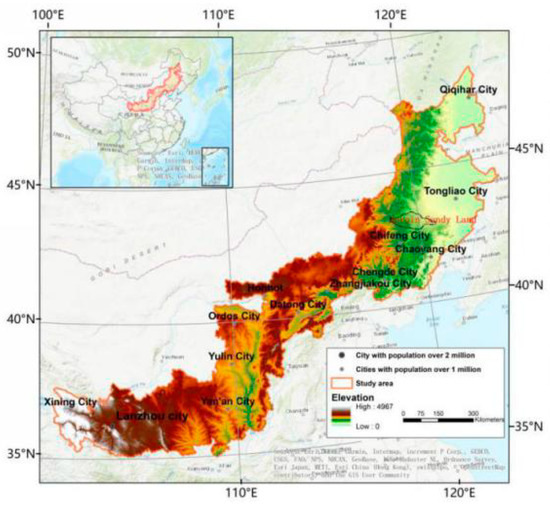
Figure 1.
Study area.
2.2. Data Preparation
In this study, many data sets were used to generate future ecological effects. Meteorological data, including daily precipitation, temperature, wind speed, and solar radiation, were acquired from the China Meteorological Administration (CMA, http://www.cma.gov.cn), comprising the period from 1977 to 2016, and then interpolated into raster maps to drive the Terrestrial Ecosystem Simulator (TES) in the Terrestrial Ecosystem Simulator-Land Use/land Cover model (TES-LUC, see Section 2.4). In terms of the input data for the land use allocation module in the TES-LUC, the initial land use map for the year 2010, and future land-use “demand” were derived from Li et al., [49] (data set available online at http://www.geosimulation.cn/GlobalLUCCProduct.html). The LULC classes include six classes: four natural land cover classes (grassland, forest, water body, and barren; especially, bare land mainly includes desert or sparsely vegetated land; Li et al., 2017), and two land use classes (cropland and built-up). Regional digital elevation models with a 30-m resolution and the soil property data were obtained from the Resource and Environment Science and Data Center (http://www.resdc.cn) and was used to obtain topographical variables (i.e., elevation and slope). Demographic data was collected from statistical yearbooks covering from 2005 to 2015, from the National Bureau of Statistics of China (http://www.stats.gov.cn). Spatial variables were resampled to 10 km by using ArcGIS (version 10.2).
2.3. Scenarios Development
We utilized the existing data-set, the LULC change projection scenarios, developed by Li et al., [49], based on four future socioeconomic scenarios (A1B, A2, B1, and B2) documented in the IPCC SRES [47,65,66]. The IPCC SRES describes alternative developments driven by forces of greenhouse gas emissions, including population, economics, technological innovation, and energy use (Figure 2). The scenarios comprised of qualitative descriptions of future conditions, often referred to as narrative storylines, and quantitative modeling, including projections of land use. The two reasons to adopt the dataset are: (1) The SRES scenarios were down-scaled using an Integrated Assessment Model in combination with a Future Land Use Simulation Model (FLUS) [60], Landsat-based land use historical trajectory, and expert knowledge. Hence, a finer resolution of LULC could match better with the ecological processes. (2) The changes in the built-up that are ignored in the IMAGE were calibrated in the data set, which can reflect the reality of economic development in our study area better.
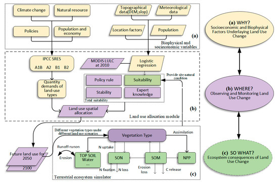
Figure 2.
Overview of the data flow in the Terrestrial Ecosystem Simulator-Land Use/land Cover model (TES-LUC). (a) is driving factors, including biophysical and socioeconomic variables. (b) is the land use allocation module; (c) is Terrestrial Ecosystem simulator. Note: Land use allocation module (b) is redrawn according to Li et al., [49]; (c) is modified from Gao et al., [56]; the coupling relationship is drawn based on Xu et al., [67]. The ellipses on the right are modified from a Framework for Assessing Multiple Ecosystem Responses to Land-Use Change [68].
Although the narrative storylines of the four scenarios have been described in detail [48,49], here we emphasize some key characteristics of each scenario. A was used to represent an economic emphasis, and on the contrary, B indicates an environmental protection; 1 denotes globalization, and 2 denotes a regional orientation.
- A1B: Low population growth; High gross domestic productivity (GDP) growth; Sprawling urban expansion; Rapid technological innovation; Energy sector—Balanced; Active management of resources.
- A2: High population growth; Low GDP growth; Sprawling urban expansion; Slow technological innovation; Energy sector—Fossil fuels; Low resources protection.
- B1: Low population growth; High GDP growth; Compact urban expansion; Rapid technological innovation; Energy sector—Renewable; Protection of biodiversity.
- B2: Medium population growth; Medium GDP growth; Compact urban expansion; Medium technological innovation; Energy sector—Mixed; Protection of biodiversity.
2.4. Land Use Allocation and Ecosystem Consequences
The Terrestrial Ecosystem Simulator-Land Use/land Cover model (TES-LUC) linked two large modules: One part is the land use allocation module (Figure 2b) and the other is TES (including NPP modules, water movement modules, ERO, and C and N cycle modules, Figure 2c). The calibration and validation of the coupling model was done in [67]. First, we extracted the quantity demands of land-use sectors from the existing dataset [60]. Then, the quantity demands were allocated to a specific spatial position to generate LULC spatial patterns in the land use allocation module based on the maximum suitability principle. Finally, the LULC spatial patterns were given as input into the process-based TES, and then the module was run to obtain explicit ecological effects.
2.4.1. Land Use Allocation Module
In this study, we adopted the framework of the conversion of land use and its effects (CLUE), which considers the natural suitability and policy restrictions. Through iterative, all the spatial units (grid cells) would be allocated a certain land use and land cover type [69,70,71,72]. Five types of land use categories (cropland, grasslands, forests, built-up, and bare land) were allocated in the module in APTZNC. In order to simplify the land-use allocation, water bodies’ changes were not considered. It was assumed that water areas remain unchanged in representing land-use dynamics. Since (i) according to the actual situation of the study area, the proportion of water is very small, only 0.1%; (ii) research focuses on changes in agricultural land (i.e., arable land, woodland, grassland) and non-agricultural land (i.e., built-up) and their impact on ecosystem functions.
Equation (1) was adopted to assign a specific land use and land cover type to each spatial unit (grid cell) with the maximum overall suitability:
where LU(r) denotes one land use and land cover type, r represents the rth grid cell, and LTj is the numerical code of land use type, LTj = 1, 2, 3, 4, and 5 for arable land, grasslands, forests, built-up, and bare land, respectively. Fsite,j is a site occurrence probability (Equation (2)). Fexpt,j is the suitability factor (Equations (3) and (4)). Floss,j is land use stability. Dj is the constants for model interactives. Each land unit (grid cell) will then be assigned a land type that has the maximum suitability and stability, and adjusted by the quantitative demand.
Binary logistic regression was used to identify the probability of events’ occurrence, which could explain the appearance of a specific land use type driven by site conditions. The advantage is that the variables can be either continuous or categorical. Fsite,j was computed as follows:
where j represents the jth land use type. Xξ for ξ from 1 to 9 denotes a series of site variables: socioeconomic variable (population density), geographical, and ecological variables (elevation, slope, average annual temperature, average annual rainfall, cumulative daily mean temperature during the growing season, rainfall during the growing season, average organic matter content of soil and average total nitrogen content of soil). aj and bjξ were regression coefficients.
Fexpt,j was calculated using Equations (3) and (4):
where wi is the weight estimated by the relationship between land use type and the ith socio-economic and ecological conditions xi. fi(xi) is the fuzzy membership function to estimate the site suitability. xi0 and Bi are parameters set up based on empirical experts’ knowledge and land classification from Food and Agriculture Organization.
Floss,j was used to quantify the stability of land use and land cover change. At least two maps of land use for different time periods were used to calculate the probability that land use type i converted to land use type j:
where µij is equal to the number of grid cells that converted to land use type j in the later map divided by the total number of grid cells that the land use type was i in the earlier map. q is the number of land use conversion trajectories.
2.4.2. Terrestrial Ecosystem Simulator
A regional ecosystem processes model (Figure 2c) was employed to obtain NPP, SOM, TN, and ERO explicitly in the APTZNC. The driving factors are meteorological data, soil and geo-spatial attributes, and the related physiological parameters of different land use types. Using different input parameters, the ecosystem functions under different land use spatial patterns could be obtained. Parametrization, validation, and the application of formulations were specifically described earlier [46,47,56]. The TES serves to quantify the four ecosystem functions based on alternative LULC scenarios.
2.5. Processes of Results Analysis
The basic analysis unit was a pixel with a resolution of 1-km. Multi-phase images were all geo-registered, and pixels at the same location in the multi-phase images can ensure spatial matching. The area of different land use types in different scenarios was calculated by the aggregation (average) of multiple pixels belonging to the same land use type. The mutual transfers between land use types indicate that the pixels in the same location might be transformed into the other five categories or remain unchanged in the next period. The pre-matrix and post-matrix were compared using MATLAB (Version 2019b) and mapped using ArcGIS (Version 10.2) to obtain land conversion maps for each scenario. Similarly, the ecosystem functions of different land use types in different scenarios were also calculated based on pixel aggregation.
3. Results
3.1. The Spatiotemporal Patterns of Land Use and Land Cover Change
The land-use spatial pattern shows significant heterogeneity in 2010 (Table 1, Figure 3a). Grassland, with the largest proportion of 74.4%, occupied the west and northwest regions with less precipitation and poorer soil condition. Cropland, accounting for 17.5%, is mostly near the eastern and southern areas, around the basins of the Yellow River, Weihe River, Fenhe River, Luanhe River, Liaohe River, and Songhua River. The forests are mainly distributed in the northeast along a sand prevention belt in the south area along the desertification-control areas, and the mountainous area, occupying 4.7%. Built-up regions are scattered in plains, intersecting with cropland and grassland.

Table 1.
Percentage of areas under different scenarios (unit: %). Figures in brackets represent changing percentage of future LULC (unit: %) compared to the year 2010 (baseline).
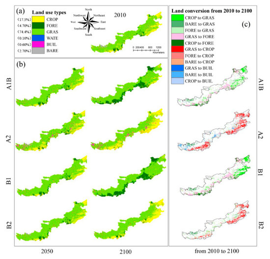
Figure 3.
Current (year 2010), future LULC maps (year 2050 and 2100), and land conversion maps from 2010 to 2100. (a) LULC map for year 2010; (b) Future LULC maps for each scenario. In the black frame of (b), the maps are arranged from left to right in order from 2050 to 2100, and arranged from top to bottom in order from A1B to B2; (c) Land conversions from 2010 to 2100 for each scenario. From top to bottom, the order is from A1B to B2. CROP = Cropland, FORE = forest, GRAS = Grassland, WATE = Water body, BUIL = Built-up, BARE = bare land.
Substantial LULC changes are expected to be observed in eastern and southwestern regions from 2010 to 2100. The environmental-oriented scenarios (i.e., scenario A1B and B1) aim to protect natural systems (e.g., grassland and forest) (Figure 3c). On the one hand, A1B is similar to B1 in the land conversion pattern that eastern cropland is projected to be transferred into grassland. Grasslands in A1B and B1 in 2100 account for 79.7% and 80.2%, respectively (Table 1). The forest is projected to be converted from cropland in the southwest and grassland in the southern margin. The proportion of forest at the end of the period reaches up to 19.8% and 22.4% in A1B and B1, respectively (Table 1). On the other hand, B1 shows more intensive conversions to ecological lands than those in A1B, which could be seen in the eastern region.
The economically oriented scenarios (i.e. scenario A2 and B2) attempt to maximize the amount of human-used land (e.g., cropland) (Figure 3c). Cropland in the east is extensively reclaimed from grassland under both the A2 and B2 scenarios, reaching up to 21.4% and 26.0%, respectively. Especially in the A2 scenario, cropland converted from forest in the southern regions could also be observed and built-up expands dramatically in the central and western regions, occupying a large number of grasslands. It should be noted that under the four scenarios, bare land in the north-west (approximately north of the Lanzhou area on the map) is expected to be restored to grassland, especially in 2100.
3.2. The Dynamics of Ecological Functions
The NPP showed significant spatial heterogeneity in 2010 (Figure 4a). The high-value regions of NPP are mainly distributed in the wet northeast area. The low-value areas of NPP were concentrated in the southeast, central, and western regions (Figure 4b). The hot points of the changes in NPP were primarily located in the southeast and south regions (Figure 4c). Comparing NPP under various scenarios from 2010 to 2100, the order is B1 > A1B > baseline > B2 > A2. The NPP under the B1 scenario showed the fastest growth, reaching up to 186.31 g C m−2 a−1 in 2100 (Table 2), and the added value is more evident in the southeast region (Figure 4c). In contrast, the NPP under the A2 scenario dipped to 125.3 g C m−2 a−1 in 2100 (Table 2), appearing in the south area (Figure 4c).
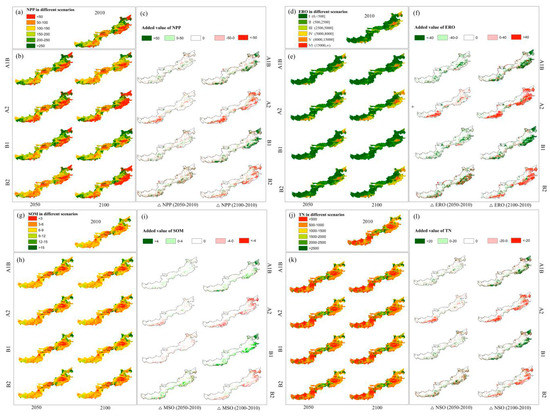
Figure 4.
Spatial distribution and added value of NPP (unit: g C m−2 a−1), ERO (unit: g m−2 a−1), SOM (unit: g kg−1), and TN (unit: mg kg−1). (a,d,g,j) are spatial distributions of NPP, ERO, SOM, and TN in year 2010. (b,e,h,k) are spatial distributions of NPP, ERO, SOM, and TN under different scenarios. In each of the four frames, the maps are arranged from left to right in order from 2020 to 2050, and arranged from top to bottom in order from A1B to B2. (c,f,i,l) are the added values of NPP, ERO, SOM, and TN from 2010 to 2050 or 2100.
Table 2.
Averaged NPP (unit: g C m−2 a−1), ERO (unit: g m−2 a−1), SOM (unit: g kg−1), and TN (unit: mg kg−1) in the landscape level under different scenarios.
In 2010, severe soil ERO were mainly distributed around the eastern Horqin sandy land and the southern Loess Plateau, whereas the areas that experienced lower erosion were in the vast northwest (Figure 4d). The hot spots of changes were in the eastern and southwestern regions (Figure 4f). The order of ERO under different scenarios is A2 > B2 > baseline > A1B > B1, which is opposite to the order for NPP. The fastest growth scenario of ERO is A2, soaring to 2930.2 g m−2 a−1 in 2100, mostly in the eastern region. However, ERO decreases greatly under the B1 scenario, decreasing to 734.1 g m−2 a−1 by the end of the period, located in the eastern and southern marginal regions.
The SOM is relatively low across the whole region (Figure 4h). In 2010, the high-value areas were mainly located in the northeast, central, and southwest regions of the APTZNC. Most of the other areas exhibited lower values (Figure 4i). The hotspots of changes were the northeast and the south (Figure 4j). The order of SOM under different scenarios is B1 > A1B > baseline > B2 > A2. The significant rise in SOM is under the B1 scenario, increasing to 9.3 g kg−1 in 2100 and the dramatic decrease trend is under the A2 scenario with 7.98 g kg−1 in 2100. Under the B1 and A1B scenarios, SOM in the northeast increases and the southern edge also shows a slightly increasing trend. In the eastern and southwestern regions under the A2 and B2 scenarios, SOM is expected to decrease. Long-term farming activities lead to a continuous decline in SOM. Comparing with the SOM in 2010, that in 2050 reduced by 1.2%, yet that in 2100 reduced by 8.1%.
3.3. Impacts of Land Use and Land Cover Dynamics on Ecological Functions
3.3.1. Impacts of Land Use and Land Cover Types on Ecological Functions
The cultivated land has the smallest NPP, SOM, and TN, and the largest ERO in 2010. Among the different ecosystem types in 2010 (Figure 5), NPP changed from 72.94 g C m−2 a−1 in cropland to 173.05 g C m−2 a−1 in forest; ERO changed from 1028.89 g m−2 a−1 in grassland to 4988.62 g m−2 a−1 in cropland; SOM varied from 7.54 g kg−1 in cropland to 9.26 g kg−1 in forest; and the change in TN ranged from 1118.97 mg kg−1 in cropland to 1245.92 mg kg−1 in forest.
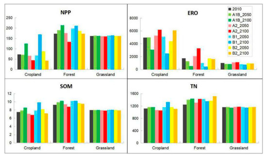
Figure 5.
Averaged NPP (unit: g C m−2 a−1), ERO (unit: g m−2 a−1), SOM (unit: g kg−1), and TN (unit: mg kg−1) in different ecosystem types under different scenarios.
The NPP of cropland is the least while that of forest is the highest under the same scenario (Figure 5). Additionally, among the different scenarios, both land use types change greatly while the grassland is relatively stable; the maximum NPP of cropland is expected to appear under the B1 scenario with 169.43 g C m−2 a−1 in 2100.
In cropland, ERO is the strongest in the same climate scenario, whereas grassland only suffers from a lower rate of ERO (Figure 5). The A2 scenario has the largest soil erosion, followed by the B2 scenario. Different ecosystem types will result in different ERO because of the close relationship between vegetation and ERO.
Under the same climate scenario, among different ecosystem types, SOM in forest is the largest and it is the smallest in cropland (Figure 5). Comparing SOM under different scenarios in the same ecosystem type, SOM in grassland is relatively stable. In forest and cropland, the SOM and TN are the largest under the B1 scenario and are the smallest under the A2 scenario.
3.3.2. Impacts of Land Use and Land Cover Conversions on Ecological Functions
Reclamation into cropland will reduce the NPP and exacerbate ERO and the loss of soil nutrients. Conversely, returning farmland to forests or grasses will increase the NPP while conserving soil (Figure 6). In the A2 and B2 scenarios, the grassland was reclaimed into cropland and the NPP decreased by 16.7 g C m−2 a−1 per decade. The soil erosion modulus increases by 600 g m−2 a−1 per decade. The average SOM decreased by 0.38 g kg−1 per decade and the TN decreased by 2.36 mg kg−1 per decade. After returning from farmland, the NPP under different scenarios increased and that under the A1B and B1 scenarios increased significantly. SOM increased by an average of 0.408 and 0.445 g kg−1 per decade after returning farmland to grassland and forest, respectively. Forests and grasslands returned from farmland have the potential to return to pre-degradation levels.
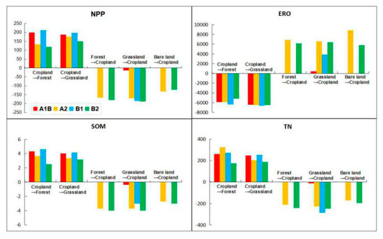
Figure 6.
The added value of NPP (unit: g C m−2 a−1), ERO (unit: g m2 a−1), SOM (unit: g kg−1), and TN (unit: mg kg−1) from 2010 to 2100 caused by LULC changes.
3.4. The Trade-Offs between Different Ecosystem Functions in 2010
Higher vegetation productivity and fertile soil meant less erosion of the soil by wind and water in the APTZNC. We explored the inherent trade-offs among multiple ecosystem functions. The relationships between NPP, SOM, and TN showed a constrained trend against ERO (Figure 7). The constraint effects of the paired ecosystem functions of NPP-ERO, SOM-ERO, and TN-ERO were similar. On the constraint lines (red line in Figure 7), ERO decreased logarithmically when NPP or SOM or TN increased on the landscape level. The responses among ecosystem functions are non-linear, such that small changes in vegetation or soil generate a large response, or vice versa.
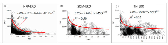
Figure 7.
The trade-offs between different ecosystem functions on the landscape level. The relationships between (a) NPP (unit: g C m−2 a−1) and ERO (unit: g m−2 a−1), (b) SOM (unit: g kg−1) and ERO (unit: g m−2 a−1), and (c) TN (unit: mg kg−1) and ERO (unit: g m−2 a−1) in 2010.
4. Discussion
4.1. What Are the Spatial Patterns of Land Use and Land Cover under Different Scenarios?
The A2 and B2 scenarios showed a significant increase in the cropland and built-up area at the cost of constant environmental deterioration during 2010–2100. Compared with the A2 and B2 scenarios, the environment-oriented A1B scenario demonstrated a slower rate of urbanization with a rapid boost in rangeland and woodland, because of the replacement of cultivated land and rangeland with woodland as well as the effective ecological conservation policies, for example, Grain for Green Program, and 2001–2050 National Grassland Ecology Protection and Construction Program. The B1 scenario is in accordance with the environment-oriented A1B scenario. Although facing a range of trajectories of future LULC, a great quantity of previous studies have reached comparable agreement concerning plausible future LULC scenarios under the IPCC SRES scenario at local and regional scales [72,73]. Concerning A2 as an illustration, they believed that the growing requirement of a bigger residential space, and weaker spatial planning is expected to frequent, as well as intensive land use conversion [74,75,76]. As to B1, it was expected that land use conversion per capita would decrease and urban sprawl would minimize, benefiting from more stringent spatial planning management, high fuel prices, and attractiveness of medium-sized cities with convenient public transportation connecting to larger cities [76].
Without concerning the IPCC SRES storyline employed, plenty of previous studies reported that a large reduction in agricultural land results from the decoupling between population growth and increase in agricultural production due to agro-technological development [66]. Besides, under all the four scenarios, sandy land and sparsely vegetated land in the north-west region in the vicinity of Lanzhou city are expected to be restored to grassland, especially in 2100. Some research reported that the vegetation in sand desert is relatively insensitive to the climate change compared to other sub-regions in APTZNC, possibly because of its high tolerance of extreme climate [77], and its previous adaption to a dry and cold environment, like water shortages [78]. Therefore, under environmental protection scenarios (A1B, B1), the demands for ecological lands are expected to increase. The sparsely vegetated land in arid areas in the west may be easily restored to grassland since the grasslands in the eastern water-rich areas may be replaced by woodland. Furthermore, under scenarios A2 and B2, the bare land also might be converted to grassland since some high-quality grasslands are occupied by urban land. This implies that although the quantity of ecological land has reached the demand, land planners and policy makers should pay more attention to the quality of ecological land.
The demand for sunlight, temperature, and water of different land use types has shaped the current spatial heterogeneity. Grasslands are predominately found in the arid and semiarid regions of the Inner Mongolian with less precipitation. Agricultural crops have high solar and water requirements; thus, they are distributed in humid areas in the east. They predominantly feature flat terrain, better natural ecological conditions, superior irrigation condition, and highly concentrated populations. Forests have played a role in windbreak and sand fixation, which are mainly distributed in the edge forest areas, especially after the implementation of regional afforestation policies.
4.2. What Are the Major Consequences of LULC for Ecosystem Functions in the Future?
The dynamics of cropland has an important impact on agro-ecosystem functions, such as food production and soil nutrient. We found that long-term agricultural land reclamation and farming practices have reduced the soil nutrient. Many studies have shown that in the southeastern part of the APTZNC, SOM drops by 0.248 g kg−1 per decade, TN decreases by 2.54 mg kg−1 per decade [79], and in the northeast of the APTZNC, SOM in black soil drops by 0.31 g kg−1 per decade [54]. After 130 years of development, the SOM content was maintained at a stable level [54]. In our study, the rate of loss in SOM is slightly higher in the next 80 years under the A1B and B1 scenario, which could have resulted from the increase in ERO in the future and the increase in the reclamation area. The main reasons are as follows: Firstly, the agricultural activities have accelerated the loss of SOM. In agricultural land, farming activities, such as reclamation, tillage, and weeding, have improved the soil microbial living environment, making it easier to decompose vegetation, roots, and residues, thereby accelerating the mineralization of organic carbon [80,81]. Secondly, due to the exposed surface of cropland, especially in the windy spring, the surface SOM is vulnerable to wind, leading to ERO [82]. Thirdly, because of the harvest, the input of SOM is reduced [83]. It indicates that after a certain period of cultivation, the cropland with low SOM may fall to a land use mode that is not suitable for continued cultivation. Therefore, in the evaluation and planning of land use, the loss of soil nutrient content caused by continuous tillage is an important indicator to be considered.
The ERO across APTZNC was in a mildly eroded level in 2010, whereas that in cropland reached a severe level. When vegetation coverage reduced, the surface roughness also reduced correspondingly [84,85]. In addition, the reduced amount of underground roots could barely fix the soil and prevent ERO [86,87]. In the areas with lower SOM and TN, the soil aggregate structure is susceptible to water erosion and wind erosion, which is then stripped and transported [88,89]. For example, in the A2 and B2 scenarios, croplands account for 33.3% and 26.0%, respectively, resulting in a large averaged ERO in the APTZNC. Not only is the cropland under human disturbance, but the bare land also contributes a lot of ERO, especially in the vicinity of Horqin sandy land, which suffers the most serious soil erosion under all of the four scenarios.
The minimum NPP appears in cropland under various scenarios, especially under the A2 scenario. Firstly, the cropland under the A2 scenario is mainly distributed in the relatively dry and barren southwestern region, where there is the desert steppe, and the adaptability of crops is poor compared to grass under this kind of condition. Therefore, after the expansion of the cropland, the averaged NPP in the APTZNC is expected to reduce. Secondly, the built-up area expands with a reduction in forest area, resulting in the smallest averaged NPP under the A2 scenario. It should be noted that under the B1 scenario, NPP of cropland is the largest in 2100, because the cropland is found in sporadic patches primarily in the northeastern regions with better water and nutrient conditions. Moreover, the proportion of forest and grassland is much larger, contributing to a higher averaged NPP in the APTZNC.
4.3. What Are the Implications of Mitigation and Adaptation Strategies to Climate Changes?
SOM is relatively stable in grassland ecosystems and could make an important contribution to effectively mitigate global climate change. Taking advantage of the carbon sequestration potential of natural ecosystems, especially of the grassland ecosystem—the main LULC in the APTZNC—could help in effectively mitigating regional climate change. Some scholars have studied the APTZNC in the city of Hohhot and found that the most active and fast-cycling component in soil organic carbon is the readily oxidizable carbon, a sensitive indicator of SOM dynamics, which can reflect the early changes of SOM [90,91]. The SOM in grassland is higher, whereas the readily oxidizable carbon is lower instead [92]. Thus, the dynamics of SOM in grassland is more stable.
Returning farmland to forests and grasses will increase soil carbon sinks and reduce soil erosion. Related studies have shown that the carbon sequestration capacity of grassland is 110 kg hm−2. The SOM of grassland increased by 0.1%, and the carbon sink increased by 600 million tons correspondingly, which is equivalent to reducing CO2 emissions by 400 million tons.
Reasonable land use practices could effectively mitigate and adapt to climate change in the APTZNC. Grazing is one of the main uses of grassland. Firstly, priority should be given to the central areas suitable for grassland, avoiding desert steppe with less precipitation and poor nutrients in the west. Secondly, the introduction of leguminous grasses can promote pasture production and thus significantly increase the soil carbon content. Re-establishment of perennial grasses will eventually improve systems to the condition with high N availability and soil stability in semiarid grassland [93,94,95]. Increased aboveground biomass, especially of rhizomatous perennial grasses, might reduce the nutrient loss, and improve forage quality [96], and increase grassland resilience to precipitation variability [97].
4.4. Can Trade-Offs between Intended and Unintended Consequences of Land Use Be Quantified to Inform Planning and Decision-Making?
Ecosystems are complex and dynamic; thus, it is impossible to respond linearly to land use changes. Small changes in vegetation or soil generate a large response, or vice versa. Returning farmland to forests and grasses could reduce soil erosion. The relationships between NPP, SOM, and TN showed a constraint trend against ERO. A study carried out in Xilin Gol League in the APTZNC has also shown that when the vegetation coverage exceeds 60%, soil erosion almost ceases [9]. Generally, vegetation can reduce wind speed, and the roots of plants can enhance soil erosion resistance. Therefore, a small increase in surface vegetation coverage and increased soil nutrients are largely conducive to controlling soil erosion. In the absence of information on ecosystem responses, it is difficult to take them into account and to weigh the trade-offs [68]. So, more studies need to be done to identify the ecosystem responses, and it becomes possible to analyze the trade-offs, non-linearities, and thresholds, which can benefit land planning and decision-making.
4.5. Limitation and Prospects
In terms of data and technology, scenarios’ development always entails many limitations and uncertainties [66]. In our work, extrapolating the observed data to future projections would introduce errors under the four scenarios since fine-resolution and local projected meteorological data are rare and inaccessible in APTZNC. So, some down-scaling exercises with the Weather Research and Forecasting Model (WRF) or Statistical Down Scaling Model (SDSM) could be operated to localize large-scale climate conditions to the region context to improve the data accuracy and reduce uncertainty. In the land use allocation module, more socioeconomic factors, like emigration/immigration, could be integrated to address more influences of human activities, especially in the larger scale research. In our further study, employing a process-based ecosystem model, researching to compare (i) the synergy effects of climate and land use on ecosystem functions, and (ii) their relative contributions are proposed to better understand the response of ecosystems.
5. Conclusions
The environmentally oriented scenarios (A1B and B1) are expected to experience marked increases in natural land covers. The economically oriented scenarios (A2 and B2) are expected to experience a significant loss of natural land covers and expansion of agricultural and urban land uses. These land conversion hotspots are mainly in the eastern and southern regions of the Agro-Pastoral Transitional Zone of Northern China. The impact of land use change on ecosystem function is related to the types of ecosystem and alternative scenarios. The general trend in net primary productivity, soil organic matter, and soil total nitrogen under the four scenarios is B1 > A1B > baseline > B2 > A2, and that in ERO is A2 > B2 > baseline > A1B > B1. The net primary productivity and soil nutrients are the largest while the soil erosion is the lightest in the woodland; the trend in cultivated land is opposite to that in woodland. Grassland protection is a priority. Grassland ecosystem functions are expected to be relatively stable and could make an important contribution to effectively alleviating global climate change. Returning farmland to forests and grasslands is an effective way to reduce carbon emissions and control land degradation, and still needs to be encouraged in the APTZNC. Besides, trade-offs between intended and unintended consequences of land use can be quantified to inform planning and decision-making.
Author Contributions
X.X. conceived, designed, and performed the experiments; H.J. and M.G. analyzed the data; L.W., T.Z., S.Q. contributed materials and analysis tools; X.X. and H.J. wrote the paper. All authors have read and agreed to the published version of the manuscript.
Funding
This research was funded by The National Key R&D Program of China, grant number 2017ZX07301-001-03, 2017YFA0604902, The Foundation for Innovative Research Groups of the National Natural Science Foundation of China, grant number 41621061, Project Supported by State Key Laboratory of Earth Surface Processes and Resource Ecology.
Conflicts of Interest
There is no conflict of interest. The founding sponsors had no role in the design of the study; in the collection, analyses, or interpretation of data; in the writing of the manuscript, and in the decision to publish the results.
References
- Turner, B.L.; Meyer, W.B.; Skole, D.L. Global Land-Use/Land-Cover Change: Towards an Integrated Study. Ambio 1994, 23, 91–95. [Google Scholar]
- Parker, D.C.; Manson, S.M.; Janssen, M.A.; Hoffmann, M.J.; Deadman, P. Multi-Agent Systems for the Simulation of Land-Use and Land-Cover Change: A Review. Ann. Assoc. Am. Geogr. 2003, 93, 314–337. [Google Scholar] [CrossRef]
- Wu, J.; He, C.; Zhang, Q.; Yu, D.; Huang, Q. Integrative modeling and strategic planning for regional sustainability under climate change. Adv. Earth Sci. 2014, 29, 1315–1324. [Google Scholar]
- Touseef, M.; Chen, L.; Masud, T.; Khan, A.; Yang, K.; Shahzad, A.; Ijaz, M.W.; Wang, Y. Assessment of the Future Climate Change Projections on Streamflow Hydrology and Water Availability over Upper Xijiang River Basin, China. Appl. Sci. 2020, 10, 3671. [Google Scholar] [CrossRef]
- Foley, J.A.; Ramankutty, N.; Brauman, K.A.; Cassidy, E.S.; Gerber, J.S.; Johnston, M.; Mueller, N.D.; O’Connell, C.; Ray, D.; West, P.C.; et al. Solutions for a cultivated planet. Nature 2011, 478, 337–342. [Google Scholar] [CrossRef]
- Mace, G.M.; Norris, K.; Fitter, A.H. Biodiversity and ecosystem services: A multilayered relationship. Trends Ecol. Evol. 2012, 27, 19–26. [Google Scholar] [CrossRef]
- Verburg, P.H.; Dearing, J.A.; Dyke, J.G.; Van Der Leeuw, S.; Seitzinger, S.; Steffen, W.; Syvitski, J. Methods and approaches to modelling the Anthropocene. Glob. Environ. Chang. 2016, 39, 328–340. [Google Scholar] [CrossRef]
- Horion, S.; Ivits, E.; De Keersmaecker, W.; Tagesson, T.; Vogt, J.; Fensholt, R. Mapping European ecosystem change types in response to land-use change, extreme climate events, and land degradation. Land Degrad. Dev. 2019, 30, 951–963. [Google Scholar] [CrossRef]
- Zhao, Y.; Liu, Z.; Wu, J. Grassland ecosystem services: A systematic review of research advances and future directions. Landsc. Ecol. 2020, 35, 793–814. [Google Scholar] [CrossRef]
- Pickett, S.T.A.; Cadenasso, M.L. Landscape Ecology: Spatial Heterogeneity in Ecological Systems. Science 1995, 269, 331–334. [Google Scholar] [CrossRef]
- Alberti, M. The Effects of Urban Patterns on Ecosystem Function. Int. Reg. Sci. Rev. 2005, 28, 168–192. [Google Scholar] [CrossRef]
- Cao, Q.; Wu, J.; Yu, D.; Wang, W. The biophysical effects of the vegetation restoration program on regional climate metrics in the Loess Plateau, China. Agric. For. Meteorol. 2019, 268, 169–180. [Google Scholar] [CrossRef]
- Schlesinger, W.H.; Andrews, J.A. Soil respiration and the global carbon cycle. Biogeochemistry 2000, 48, 7–20. [Google Scholar] [CrossRef]
- Houghton, R.A. Revised estimates of the annual net flux of carbon to the atmosphere from changes in land use and land management 1850–2000. Tellus Ser. B Chem. Phys. Meteorol. 2003, 55, 378–390. [Google Scholar]
- Xu, X.; Jiang, H.; Tian, X.; Guan, M.; Wang, L. Response of the Plant and Soil Features to Degradation Grades in Semi-arid Grassland of the Inner Mongolia, China. IOP Conf. Ser. Mater. Sci. Eng. 2019, 484, 012039. [Google Scholar] [CrossRef]
- Zhang, Q.; Kong, D.; Singh, V.P.; Shi, P. Response of vegetation to different time-scales drought across China: Spatiotemporal patterns, causes and implications. Glob. Planet Chang. 2017, 152, 1–11. [Google Scholar] [CrossRef]
- McDonagh, J.; Birch-Thomsen, T.; Magid, J. Soil organic matter decline and compositional change associated with cereal cropping in southern Tanzania. Land Degrad. Dev. 2001, 12, 13–26. [Google Scholar] [CrossRef]
- Fazhu, Z.; Jiao, S.; Chengjie, R.; Di, K.; Jian, D.; Han, X.; Gaihe, Y.; Yongzhong, F.; Guangxin, R. Land use change influences soil C, N and P stoichiometry under ‘Grain-to-Green Program’ in China. Sci. Rep. 2015, 5, srep10195. [Google Scholar] [CrossRef]
- Wang, J.; Peng, J.; Zhao, M.; Yanxu, L.; Chen, Y. Significant trade-off for the impact of Grain-for-Green Programme on ecosystem services in North-western Yunnan, China. Sci. Total Environ. 2017, 574, 57–64. [Google Scholar] [CrossRef]
- McGarigal, K.; Marks, B.J. FRAGSTATS: Spatial Pattern Analysis Program for Quantifying Landscape Structure; USDA Forest Service: Portland, OR, USA, 1995; p. 351.
- Gustafson, E.J. Minireview: Quantifying Landscape Spatial Pattern: What Is the State of the Art? Ecosystems 1998, 1, 143–156. [Google Scholar] [CrossRef]
- Luck, M.; Wu, J. A gradient analysis of urban landscape pattern: A case study from the Phoenix metropolitan region, Arizona, USA. Landsc. Ecol. 2002, 17, 327–339. [Google Scholar] [CrossRef]
- Wu, J. Effects of changing scale on landscape pattern analysis: Scaling relations. Landsc. Ecol. 2004, 19, 125–138. [Google Scholar] [CrossRef]
- Lovett, G.M.; Jones, C.G.; Turner, M.; Weathers, K.C. Ecosystem Function in Heterogeneous Landscapes. Ecosyst. Funct. Heterog. Landsc. 2007, 1–4. [Google Scholar] [CrossRef]
- Hao, R.; Yu, D.; Liu, Y.; Liu, Y.; Qiao, J.; Wang, X.; Du, J. Impacts of changes in climate and landscape pattern on ecosystem services. Sci. Total Environ. 2017, 579, 718–728. [Google Scholar] [CrossRef] [PubMed]
- Scarnecchia, D.L.; Jorgensen, S.E. Fundamentals of Ecological Modelling. J. Range Manag. 1995, 48, 566. [Google Scholar] [CrossRef]
- Gao, Q.; Yu, M.; Yang, X.; Wu, J. Scaling simulation models for spatially heterogeneous ecosystems with diffusive transportation. Landsc. Ecol. 2001, 16, 289–300. [Google Scholar] [CrossRef]
- DeAngelis, D.L.; Yurek, S. Spatially Explicit Modeling in Ecology: A Review. Ecosystems 2016, 20, 284–300. [Google Scholar] [CrossRef]
- Grimm, V.; Ayllón, D.; Railsback, S.F. Next-Generation Individual-Based Models Integrate Biodiversity and Ecosystems: Yes We Can, and Yes We Must. Ecosystems 2016, 20, 229–236. [Google Scholar] [CrossRef]
- Peters, D.P.; Okin, G.S. A Toolkit for Ecosystem Ecologists in the Time of Big Science. Ecosystems 2016, 20, 259–266. [Google Scholar] [CrossRef]
- Moloney, K.; Levin, S.A. The Effects of Disturbance Architecture on Landscape-Level Population Dynamics. Ecology 1996, 77, 375–394. [Google Scholar] [CrossRef]
- Rastetter, E.B. Modeling for Understanding v. Modeling for Numbers. Ecosystems 2016, 20, 215–221. [Google Scholar] [CrossRef]
- Turner, M.; Carpenter, S.R. Ecosystem Modeling for the 21st Century. Ecosystems 2016, 20, 211–214. [Google Scholar] [CrossRef]
- Potter, C.; Randerson, J.T.; Field, C.B.; Matson, P.A.; Vitousek, P.M.; Mooney, H.A.; Klooster, S.A. Terrestrial ecosystem production: A process model based on global satellite and surface data. Glob. Biogeochem. Cycles 1993, 7, 811–841. [Google Scholar] [CrossRef]
- Rafique, R.; Xia, J.; Hararuk, O.; Leng, G.; Asrar, G.; Luo, Y.; Rafique, R. Comparing the Performance of Three Land Models in Global C Cycle Simulations: A Detailed Structural Analysis. Land Degrad. Dev. 2016, 28, 524–533. [Google Scholar] [CrossRef]
- Martine, J.V.D.P.; Jantiene, E.M.B.; David, A.R. Biophysical landscape interactions: Bridging disciplines and scale with connectivity. Land Degrad. Dev. 2018, 29, 1167–1175. [Google Scholar]
- Fryrear, D.W.; Saleh, A.; Bilbro, J.B. A single event wind erosion model. Trans. ASAE 1998, 41, 1369. [Google Scholar] [CrossRef]
- Borrelli, P.; Lugato, E.; Montanarella, L.; Panagos, P. A New Assessment of Soil Loss Due to Wind Erosion in European Agricultural Soils Using a Quantitative Spatially Distributed Modelling Approach. Land Degrad. Dev. 2016, 28, 335–344. [Google Scholar] [CrossRef]
- Parton, W.J.; Schimel, D.; Cole, C.V.; Ojima, D.S. Analysis of Factors Controlling Soil Organic Matter Levels in Great Plains Grasslands. Soil Sci. Soc. Am. J. 1987, 51, 1173–1179. [Google Scholar] [CrossRef]
- Parton, W.J.; Stewart, J.W.B.; Cole, C.V. Dynamics of C, N, P and S in grassland soils: A model. Biogeochemistry 1988, 5, 109–131. [Google Scholar] [CrossRef]
- Parton, W.J.; Neff, J.; Vitousek, P.M. Modelling phosphorus, carbon and nitrogen dynamics in terrestrial ecosystems. Org. Phosphorus Environ. 2005. [Google Scholar] [CrossRef]
- Running, S.W.; Coughlan, J.C. A general model of forest ecosystem processes for regional applications I. Hydrologic balance, canopy gas exchange and primary production processes. Ecol. Model. 1988, 42, 125–154. [Google Scholar] [CrossRef]
- Running, S.W.; Hunt, E.R. Generalization of a Forest Ecosystem Process Model for Other Biomes, BIOME-BGC, and an Application for Global-Scale Models. Scaling Physiol. Proc. 1993, 141–158. [Google Scholar] [CrossRef]
- Churkina, G.; Running, S.W. Contrasting Climatic Controls on the Estimated Productivity of Global Terrestrial Biomes. Ecosystems 1998, 1, 206–215. [Google Scholar] [CrossRef]
- Sanchez-Ruiz, S.; Chiesi, M.; Fibbi, L.; Carrara, A.; Maselli, F.; Gilabert, M. Optimized Application of Biome-BGC for Modeling the Daily GPP of Natural Vegetation Over Peninsular Spain. J. Geophys. Res. Biogeosci. 2018, 123, 531–546. [Google Scholar] [CrossRef]
- Jiang, H.; Xu, X.; Guan, M.; Wang, L.; Huang, Y.; Jiang, Y. Determining the contributions of climate change and human activities to vegetation dynamics in agro-pastural transitional zone of northern China from 2000 to 2015. Sci. Total Environ. 2020, 718, 134871. [Google Scholar] [CrossRef]
- Nakicenovic, N.; Alcamo, J.; Davis, G.; Vries, B.D. Special Report on Emissions Scenarios: A Special Report of the Working Group III of the Intergovernmental Panel on Climate Change; Cambridge University Press: Cambridge, UK, 2000. [Google Scholar]
- Sleeter, B.M.; Sohl, T.L.; Bouchard, M.A.; Reker, R.R.; Soulard, C.E.; Acevedo, W.; Griffith, G.E.; Sleeter, R.R.; Auch, R.F.; Sayler, K.L.; et al. Scenarios of land use and land cover change in the conterminous United States: Utilizing the special report on emission scenarios at ecoregional scales. Glob. Environ. Chang. 2012, 22, 896–914. [Google Scholar] [CrossRef]
- Li, X.; Yu, L.; Sohl, T.; Clinton, N.; Li, W.; Zhu, Z.; Liu, X.; Gong, P. A cellular automata downscaling based 1 km global land use datasets (2010–2100). Sci. Bull. 2016, 61, 1651–1661. [Google Scholar] [CrossRef]
- Luoto, M.; Virkkala, R.; Heikkinen, R.K. The role of land cover in bioclimatic models depends on spatial resolution. Glob. Ecol. Biogeogr. 2007, 16, 34–42. [Google Scholar] [CrossRef]
- Di Febbraro, M.; Menchetti, M.; Russo, D.; Ancillotto, L.; Aloise, G.; Roscioni, F.; Preatoni, D.; Loy, A.; Martinoli, A.; Bertolino, S.; et al. Integrating climate and land-use change scenarios in modelling the future spread of invasive squirrels in Italy. Divers. Distrib. 2019, 25, 644–659. [Google Scholar] [CrossRef]
- Strayer, D.L.; Beighley, R.E.; Thompson, L.C.; Brooks, S.; Nilsson, C.; Pinay, G.; Naiman, R.J. Effects of land cover on stream ecosystems: Roles of empirical models and scaling issues. Ecosystems 2003, 6, 407–423. [Google Scholar] [CrossRef]
- Milano, M.; Reynard, E.; Köplin, N.; Weingartner, R. Climatic and anthropogenic changes in Western Switzerland: Impacts on water stress. Sci. Total Environ. 2015, 536, 12–24. [Google Scholar] [CrossRef] [PubMed]
- Yu, J.; Liu, J.; Wang, J.; Liu, S.; Qi, X.; Wang, Y.; Wang, G. Organic Carbon Variation Law of Black Soil During Different Tillage Period. J. Soil Water Conserv. 2004, 18, 27–30. [Google Scholar]
- Pielke, R.A.; Marland, G.; Betts, R.A.; Chase, T.N.; Eastman, J.L.; Niles, J.O.; Niyogi, D.D.S.; Running, S.W. The influence of land-use change and landscape dynamics on the climate system: Relevance to climate-change policy beyond the radiative effect of greenhouse gases. Philos. Trans. R. Soc. A Math. Phys. Eng. Sci. 2002, 360, 1705–1719. [Google Scholar] [CrossRef] [PubMed]
- Gao, Q.; Yu, M.; Liu, Y.; Xu, H.; Xu, X. Modeling interplay between regional net ecosystem carbon balance and soil erosion for a crop-pasture region. J. Geophys. Res. Space Phys. 2007, 112, 112. [Google Scholar] [CrossRef]
- Heistermann, M.; Müller, C.; Ronneberger, K. Land in sight?Achievements, deficits and potentials of continental to global scale land-use modeling. Agric. Ecosyst. Environ. 2006, 114, 141–158. [Google Scholar] [CrossRef]
- Sohl, T.L.; Sayler, K.L.; Bouchard, M.A.; Reker, R.R.; Friesz, A.M.; Bennett, S.L.; Sleeter, B.M.; Sleeter, R.R.; Wilson, T.S.; Soulard, C.; et al. Spatially explicit modeling of 1992–2100 land cover and forest stand age for the conterminous United States. Ecol. Appl. 2014, 24, 1015–1036. [Google Scholar] [CrossRef]
- Wilson, T.S.; Sleeter, B.M.; Davis, A.W. Potential future land use threats to California’s protected areas. Reg. Environ. Chang. 2014, 15, 1051–1064. [Google Scholar] [CrossRef]
- Liu, X.; Liang, X.; Li, X.; Xu, X.; Ou, J.; Chen, Y.; Li, S.; Wang, S.; Pei, F. A future land use simulation model (FLUS) for simulating multiple land use scenarios by coupling human and natural effects. Landsc. Urban Plan. 2017, 168, 94–116. [Google Scholar] [CrossRef]
- Wang, J.; Xu, X.; Liu, P. Land use and land carrying capacity in ecotone between agriculture and animal husbandry in northern China. Resour. Sci. 1999, 21, 19–24. [Google Scholar]
- Shi, P. Pattern and Optimization Simulation of Land Use in Pastoral Transitional Zone in Northern China; Science Press: Beijing, China, 2009. [Google Scholar]
- Jiang, H.; Xu, X.; Guan, M.; Wang, L.; Huang, Y.; Liu, Y. Simulation of Spatiotemporal Land Use Changes for Integrated Model of Socioeconomic and Ecological Processes in China. Sustainability 2019, 11, 3627. [Google Scholar] [CrossRef]
- Huang, D.; Wang, K.; Wu, W. Problems and strategies for sustainable development of farming and animal husbandry in the Agro-Pastoral Transition Zone in Northern China (APTZNC). Int. J. Sustain. Dev. World Ecol. 2007, 14, 391–399. [Google Scholar] [CrossRef]
- Gaffin, S.R.; Rosenzweig, C.; Xing, X.; Yetman, G. Downscaling and geo-spatial gridding of socio-economic projections from the IPCC Special Report on Emissions Scenarios (SRES). Glob. Environ. Chang. 2004, 14, 105–123. [Google Scholar] [CrossRef]
- Rounsevell, M.; Reginster, I.; Araújo, M.B.; Carter, T.; Dendoncker, N.; Ewert, F.; House, J.I.; Kankaanpää, S.; Leemans, R.; Metzger, M.; et al. A coherent set of future land use change scenarios for Europe. Agric. Ecosyst. Environ. 2006, 114, 57–68. [Google Scholar] [CrossRef]
- Xu, X.; Gao, Q.; Liu, Y.-H.; Wang, J.-A.; Zhang, Y. Coupling a land use model and an ecosystem model for a crop-pasture zone. Ecol. Model. 2009, 220, 2503–2511. [Google Scholar] [CrossRef]
- DeFries, R.S.; Asner, G.P.; Houghton, R.A. Trade-offs in land-use decisions: Towards a framework for assessing multiple ecosystem responses to land-use change. In Ecosystems and Land Use Change; Blackwell Publishing Ltd.: Oxford, UK, 2004; Volume 153, pp. 1–9. [Google Scholar]
- Veldkamp, A.; Verburg, P. Modelling land use change and environmental impact. J. Environ. Manag. 2004, 72, 1–3. [Google Scholar] [CrossRef]
- Verburg, P.H.; De Koning, G.; Kok, K.; Veldkamp, A.; Bouma, J. A spatial explicit allocation procedure for modelling the pattern of land use change based upon actual land use. Ecol. Model. 1999, 116, 45–61. [Google Scholar] [CrossRef]
- Verburg, P.H. Simulating feedbacks in land use and land cover change models. Landsc. Ecol. 2006, 21, 1171–1183. [Google Scholar] [CrossRef]
- Verburg, P.H.; Overmars, K.P. Combining top-down and bottom-up dynamics in land use modeling: Exploring the future of abandoned farmlands in Europe with the Dyna-CLUE model. Landsc. Ecol. 2009, 24, 1167–1181. [Google Scholar] [CrossRef]
- Rounsevell, M.D.A.; Reay, D.S. Land use and climate change in the UK. Land Policy 2009, 26, S160–S169. [Google Scholar] [CrossRef]
- Solecki, W.; Oliveri, C. Downscaling climate change scenarios in an urban land use change model. J. Environ. Manag. 2004, 72, 105–115. [Google Scholar] [CrossRef]
- Hansen, H.S. Modelling the future coastal zone urban development as implied by the IPCC SRES and assessing the impact from sea level rise. Landsc. Urban Plan. 2010, 98, 141–149. [Google Scholar] [CrossRef]
- Han, H.; Hwang, Y.; Ha, S.R.; Kim, B.S. Modeling Future Land Use Scenarios in South Korea: Applying the IPCC Special Report on Emissions Scenarios and the SLEUTH Model on a Local Scale. Environ. Manag. 2015, 55, 1064–1079. [Google Scholar] [CrossRef] [PubMed]
- Li, P.; Liu, L.; Wang, J.; Wang, Z.; Wang, X.; Bai, Y.; Chen, S. Wind erosion enhanced by land use changes significantly reduces ecosystem carbon storage and carbon sequestration potentials in semiarid grasslands. Land Degrad. Dev. 2018, 29, 3469–3478. [Google Scholar] [CrossRef]
- Zhang, S.; Fan, W.; Li, Y.; Yi, Y. The influence of changes in land use and landscape patterns on soil erosion in a watershed. Sci. Total Environ. 2017, 574, 34–45. [Google Scholar] [CrossRef] [PubMed]
- Jiao, Y.; Hou, J.; Zhao, J.; Yang, W. Land-use change from grassland to cropland affects CH4 uptake in the farming-pastoral ecotone of Inner Mongolia. China Environ. Sci. 2014, 34, 1514–1522. [Google Scholar]
- Lal, R. Soil carbon dynamics in cropland and rangeland. Environ. Pollut. 2002, 116, 353–362. [Google Scholar] [CrossRef]
- Hamza, M.A.; Anderson, W.K. Soil compaction in cropping systems. Soil Tillage Res. 2005, 82, 121–145. [Google Scholar] [CrossRef]
- Dorren, L.K.A.; Imeson, A.C. Soil erosion and the adaptive cycle metaphor. Land Degrad. Dev. 2005, 16, 509–516. [Google Scholar] [CrossRef]
- Fialho, R.C.; Teixeira, R.D.S.; Teixeira, A.P.M.; Da Silva, I.R. Short-term carbon emissions: Effect of various tree harvesting, transport, and tillage methods under a eucalyptus plantation. Land Degrad. Dev. 2018, 29, 3995–4004. [Google Scholar] [CrossRef]
- Rondeaux, G.; Steven, M.; Baret, F. Optimization of soil-adjusted vegetation indices. Remote Sens. Environ. 1996, 55, 95–107. [Google Scholar] [CrossRef]
- Leenders, J.K.; Sterk, G.; Van Boxel, J. Wind Erosion Reduction by Scattered Woody Vegetation in Farmers’ Fields in Northern Burkina Faso. Land Degrad. Dev. 2014, 27, 1863–1872. [Google Scholar] [CrossRef]
- Gyssels, G.; Poesen, J.; Bochet, E.; Li, Y. Impact of plant roots on the resistance of soils to erosion by water: A review. Prog. Phys. Geogr. 2005, 29, 189–217. [Google Scholar] [CrossRef]
- Guo, M.; Wang, W.; Shi, Q.; Chen, T.; Kang, H.; Li, J. An experimental study on the effects of grass root density on gully headcut erosion in the gully region of China’s Loess Plateau. Land Degrad. Dev. 2019, 30, 2107–2125. [Google Scholar] [CrossRef]
- Zobeck, T.M. Soil properties affecting wind erosion. J. Soil Water Conserv. 1991, 46, 112–118. [Google Scholar]
- Lal, R. Soil degradation by erosion. Land Degrad. Dev. 2001, 12, 519–539. [Google Scholar] [CrossRef]
- Hu, L.; Youngberg, C.T.; Gilmour, C.M. Readily Oxidizable Carbon: An Index of Decomposition and Humification of Forest Litter. Soil Sci. Soc. Am. J. 1972, 36, 959–961. [Google Scholar] [CrossRef]
- Luo, Y.; Li, Q.; Wang, C.; Li, B.; Stomph, T.J.; Yang, J.; Tao, Q.; Yuan, S.; Tang, X.; Ge, J.; et al. Negative effects of urbanization on agricultural soil easily oxidizable organic carbon down the profile of the Chengdu Plain, China. Land Degrad. Dev. 2019, 31, 404–416. [Google Scholar] [CrossRef]
- Wei, H.; Li, Z.; Zhang, L.; Li, X.; Yu, D.; Bai, X. Effects of Land Use Types on Soil Organic Carbon and Readily Oxidizable Carbon. J. Inner Mong. Univ. Natl. Nat. Sci. 2017, 15, 226–232. [Google Scholar]
- Burke, I.C.; Lauenroth, W.K.; Coffin, D.P. Soil Organic Matter Recovery in Semiarid Grasslands: Implications for the Conservation Reserve Program. Ecol. Appl. 1995, 5, 793–801. [Google Scholar] [CrossRef]
- Chen, X.; Duan, Z.; Tan, M. Restoration Affect Soil Organic Carbon and Nutrients in Different Particle-size Fractions. Land Degrad. Dev. 2015, 27, 561–572. [Google Scholar] [CrossRef]
- Zhang, Z.; Li, Q.; Zhang, H.; Hu, Y.; Hou, S.; Wei, H.; Yin, J.; Lü, X.-T. The impacts of nutrient addition and livestock exclosure on the soil nematode community in a degraded grassland. Land Degrad. Dev. 2019, 30, 1574–1583. [Google Scholar] [CrossRef]
- Schellberg, J.; Moseler, B.M.; Kuhbauch, W.; Rademacher, I.F. Long-term effects of fertilizer on soil nutrient concentration, yield, forage quality and floristic composition of a hay meadow in the Eifel mountains, Germany. Grass Forage Sci. 1999, 54, 195–207. [Google Scholar] [CrossRef]
- Bai, Y.; Han, X.; Wu, J.; Chen, Z.; Li, L. Ecosystem stability and compensatory effects in the Inner Mongolia grassland. Nature 2004, 431, 181–184. [Google Scholar] [CrossRef] [PubMed]
© 2020 by the authors. Licensee MDPI, Basel, Switzerland. This article is an open access article distributed under the terms and conditions of the Creative Commons Attribution (CC BY) license (http://creativecommons.org/licenses/by/4.0/).