An Enhanced Planar Linked Segment Model for Predicting Lumbar Spine Loads during Symmetric Lifting Tasks

Abstract

The present technical note aimed at enriching the planar linked segment model originally proposed by Chaffin with the prediction of the moment arm and of the orientation of the line of action of the back extensor muscles during symmetric lifting tasks. The prediction equations proposed by van Dieen and de Looze for their single equivalent muscle model were used for such a purpose. Their prediction was based on the thorax-to-pelvis flexion angle as computed from 3D video-based motion capture. In order to make these prediction equations compliant with a two-dimensional analysis, the planar angle formed by the segment joining L5/S1 to the shoulder with the longitudinal axis of the pelvis was introduced. This newly computed planar trunk flexion angle was used to feed van Dieen and de Looze’s equations, comparing the results with the original model. A full-body Plug-in-Gait model relative to 10 subjects performing manual lifting activities using a stoop and a squat technique was used for model validation. A strong association was found between the proposed planar trunk flexion angle and that used by van Dieen and de Looze (r = 0.970). A strong association and a high level of agreement were found between the back extensor muscle moment arm (r = 0.965; bias < 0.001 m; upper limit of agreement (LOA) = 0.002 m; lower LOA < 0.001 m) and the orientation of the line of action (r = 0.970; bias = 2.8°; upper LOA = 5.3°; lower LOA = 0.2°) as computed using the two methods. For both the considered variables, the prediction error fell within the model sensitivity.

1. Introduction

Quantifying the loads stressing the lumbar spine during manual lifting activities is crucial for assessing the risk of work-related low back pain [1,2]. Spinal loads are usually identified as the compressive and shear forces acting on one of the lumbar intervertebral disc centers. The earliest approach for the determination of such forces through indirect methods is the planar linked segment model (LSM) proposed by Chaffin in 1969 and still currently used for the analysis of static symmetric lifting activities [3].

Briefly, conventional Newtonian mechanics are sequentially applied to each body segment starting at one end of the chain (i.e., the hand) where external loads can be either known or measured. Assuming that the forces of the anatomical structures crossing the joint can be reduced to one moment and one resultant force acting at the joint center, intersegmental forces and moments are calculated at each joint of the chain to the intervertebral disc center of interest (L5/S1). Shear and compressive forces are, then, computed as the components along the S1 vertebra-fixed reference frame of the intersegmental force acting on the intervertebral disc center plus the contribution of the back extensor muscle force and of the force created by the abdominal pressure along the compressive axis only (i.e., the axis normal to the vertebral plate). The inclination of the S1 vertebral plate is computed by adding the inclination of the disc in upright posture (40°) to the sacral rotation, which is, in turn, predicted as a function of the measured trunk and knee angles [4]. Abdominal pressure is estimated as a function of the hip torque and the hip angle [5] and converted into a force by assuming a given diaphragm area [3]. Finally, the back extensor muscle force is estimated by dividing the intersegmental moment by the muscle moment arm, assuming that the back extensor muscles are represented by a single muscle equivalent and that the intersegmental moment can be attributed solely to muscle forces [6]. The back extensor muscle moment arm is retrieved from cadaveric studies, and its value, with respect to a neutral trunk orientation, is assumed to be constant regardless of the degree of trunk flexion. A detailed representation and implementation of Chaffin’s LSM model can be found in his book [7].

Chaffin’s musculoskeletal modelling has known limitations affecting the accuracy of the predicted spinal loads [6,8,9,10]. Most of these limitations have been overcome by more detailed and even subject-specific musculoskeletal models controlled by either static or dynamic optimization and fed with three-dimensional (3D) camera-based motion capture data [11,12]. Despite these limitations, Chaffin’s model is still widely used in occupational ergonomics for its affordable measurement technique (the planar positions of the joints of the LSM can be easily retrieved from an image), ease of use and the fact it is implemented in several industry-oriented commercially available software packages [9,13,14]. In fact, 3D motion capture is not easily accessible to everyone for its cost, space requirements and expertise related to its use. Moreover, 3D motion capture is hard to use on a routine basis, which is what is needed in industrial settings for risk management. Therefore, it is worthwhile to conduct more research to enhance, where possible, the model proposed by Chaffin.

Among the limitations of this approach, the fixed moment arm of the back-extensor muscles is surely a critical point, as it has been shown that applying the lever arm obtained in an upright stance to a flexed position leads to a significant underestimation and overestimation of the compression and shear forces, respectively [15]. The orientation of the muscle’s line of action (crucial for projecting the muscle force on the vertebral body properly), assumed to be parallel to the axis of compression and characterized by a constant value, has even worse effects [15]. In their single-equivalent muscle (SEM) model, van Dieen and de Looze predicted the back extensor muscle moment arm and the orientation of their line of action (with respect to the plane of L5/S1) as a function of the thorax-to-pelvis angle from 10° of trunk extension to 55° of flexion with a resolution of 5° [15] (Figure 1). The regression was based on a model consisting of 114 muscles crossing L5/S1 [16].

The aim of the present technical note is to investigate if any relation exists between the thorax angle used by van Dieen and de Looze, as computed by using 3D photogrammetry, and a functionally related angle available from the planar LSM proposed by Chaffin. If so, van Dieen’s regression equations could be used to enhance Chaffin’s model by a variable back-extensor muscle moment arm and line of action according to the subject’s posture during the lifting activity.

2. Materials and Methods

2.1. The Enhanced Chaffin’s LSM

The angle of the thorax relative to the pelvis (TP) used by van Dieen and de Looze to predict the SEM moment arm and line of action is defined as the sagittal plane component of the Euler rotation of a 3D thorax-embedded anatomical frame with respect to a 3D pelvis-embedded anatomical frame [16]. Thorax and pelvis anatomical reference systems were defined according to McConville [16,17]. Figure 2 depicts an angle functionally related to TP that is supposed to be linearly related to it. This angle (φ) is formed in the sagittal plane by the segment joining the L5/S1 joint to the shoulder joint center S and the longitudinal axis of a pelvis-embedded frame (y_pv). y_pv is perpendicular to the axis joining the posterior superior iliac spine (PSIS) anterior with the anterior superior iliac spine (ASIS).

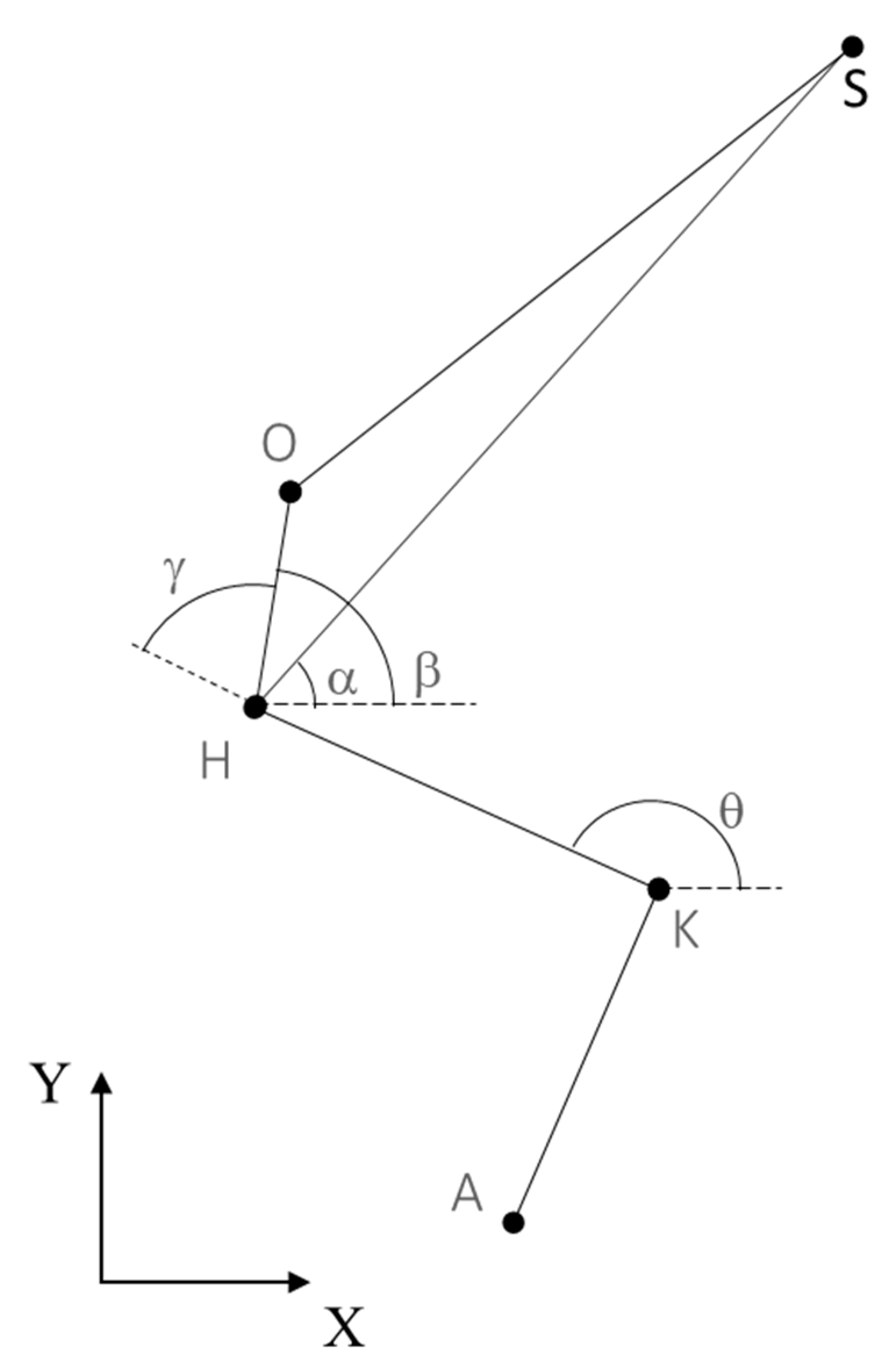
The planar Chaffin’s LSM depicted in Figure 3 and used to predict φ consists of some selected points on the subject’s body, whose position can be measured from an image through photogrammetry, and other points whose positions can be estimated by anatomical assumptions:

• The position of S can be estimated as a function of the inter-acromial distance from the position of the acromion (AC) (note that in the Chaffin’s LSM, the position of S is usually made to coincide with the position of the acromion instead) [18]. This requires the user to measure the inter-ASIS distance beforehand to analyze the task.
• The position of the hip joint center (H) can be estimated as a function of the inter-ASIS distance and pelvic width with respect to a pelvis-embedded frame [19]. This requires the user to measure the inter-ASIS distance beforehand to analyze the task, while the pelvic width can be measured by photogrammetry as the ASIS-to-PSIS distance. Note that, among all the anthropometry-based equations for predicting the hip joint center position, the equation proposed by Harrington has been proved as the most accurate [20]. However, pelvic width is originally defined as the line joining the midpoint between the right and the left ASIS and the midpoint between the right and left PSIS. Since such measures are not available in two dimensions (we can only consider either the right- or the left-sided ASIS–PSIS distance), the user may decide to use the Bell and Brand approach, which relies on the sole inter-ASIS distance [21]. H can be then expressed with respect to the global reference frame XY through a rigid transformation by using the position and orientation of the pelvis-embedded reference frame defined above.
• The planar positions of the knee (K) and ankle (A) joint centers can be assumed to correspond to the positions of the lateral femur epicondyle and of the peroneal malleolus, respectively.

Note that AC, ASIS, PSIS, K and A are all superficial and, hence, palpable anatomical landmarks, and their planar positions can be easily measured through photogrammetry (with the help of well-visible markers, for instance).

• Finally, the position of L5/S1 (labeled as O in Figure 3 for space convenience) in the absolute reference frame XY can be estimated as follows:

$${\mathrm{O}}_{\mathrm{x}}=\parallel \overrightarrow{\mathrm{HO}}\parallel ·\cos \mathsf{\beta }+{\mathrm{H}}_{\mathrm{x}}$$

(1)

$${\mathrm{O}}_{\mathrm{y}}=\parallel \overrightarrow{\mathrm{HO}}\parallel ·\sin \mathsf{\beta }+{\mathrm{H}}_{\mathrm{y}}$$

(2)

where

$$\mathsf{\beta }=\mathsf{\theta }-\mathsf{\gamma }$$

(3)

and

$$\mathsf{\gamma }=2/3·\left(\mathsf{\theta }-\mathsf{\alpha }-27\right)$$

(4)

γ is the pelvic rotation angle as defined by Chaffin [22], β is the angle formed by the segment joining H to O with the horizontal axis, and α and θ are the inclinations of the trunk and of the thigh with respect to the horizontal axis, respectively. Finally, $\parallel \overrightarrow{HO}\parallel$ corresponds to the length of the segment joining H to O that is considered to be, in an erect position, 19.5% of the measured length of the segment joining H to S (the H-to-S length can be measured from the planar positions of H and S) [7,22]. Note that α and θ can be computed from the positions of S, H, K and A.

Once the position of O is known and the vector joining H to O can be computed, the angle of interest φ can be estimated as follows:

$$\mathsf{\phi }=\arccos (\frac{\widehat{\mathrm{OS}}}{\parallel \overrightarrow{\mathrm{OS}}\parallel }\ast {\mathrm{y}}_{\mathrm{pv}})$$

(5)

where the asterisk indicates the dot product operation and y_pv is a unit vector.

Note that the estimation of the S1 vertebral plate inclination, needed to define the axes of compression and shear and which is also part of Chaffin’s LSM, is not included in this technical note, as it is not relevant to our aims, but the computational details and related assumptions can be found in Chaffin’s book [7].

From φ, the back extensor muscle moment arm (in meters) and the orientation of the line of action with respect to the plane of L5/S1 (in degrees) may be predicted by using the equations of van Dieen and de Looze [15] as follows:

$$\mathrm{moment} \mathrm{arm}=\left(\mathrm{a}·{\mathsf{\phi }}^2\right)+(\mathrm{b}·\mathsf{\phi })+\mathrm{c}$$

(6)

$$\mathrm{line} \mathrm{of} \mathrm{action}=\left(\mathrm{d}·\mathsf{\phi }\right)+\mathrm{e}$$

(7)

where a, b, c, d and e are the coefficients of the regression models found by van Dieen and de Looze [15] (

Table 1. Coefficients of the regression models proposed by van Dieen and de Looze for predicting the back extensor muscle moment arm and the orientation of the line of action as a function of the thorax-to-pelvis flexion angle.

Factor	$\mathbf{a}·{10}^{-6}$	$\mathbf{b}·{10}^{-5}$	$\mathbf{c}·{10}^{-2}$	$\mathbf{d}·{10}^{-1}$	e
Standard model	−1.9	−9.18	5.08	−5.25	129

).

2.2. Model Validation

TP and φ were computed using a dataset made available by Maurice et al. [23]. The database consists of the 3D positions of markers arranged on the subject’s body according to the full-body Plug-in-Gait marker set and collected using an infrared camera-based optoelectronic stereophotogrammetric system. The motion capture data are relative to 13 healthy adults performing a set of workplace-related tasks following 3 different sequences that were repeated 5 times by each participant. Each performed sequence included lifting a 5 kg load from a 55 cm-high table using a stoop technique and placing it down on a 20 cm-high table using a squat technique. Essentially, a total of 15 stoop and 15 squat lifts for each of the 13 participants were potentially available. Unfortunately, only a subset of the data was effectively used for data analysis: several trials were found to be characterized by the occlusion of the thorax markers needed for determining the thorax reference frame (which was, in turn, needed to compute TP). A total of 47 trials, each characterized by a stoop and a squat lift, from 10 participants were eventually used for model validation (see

Table 2. This table shows, for each participant included in Maurice et al.’s database, the number of trials effectively used for model validation.

ID	Number of Analyzed Trials
Participant_541	6
Participant_909	0
Participant_2193	1
Participant_2274	12
Participant_3327	3
Participant_5124	3
Participant_5319	3
Participant_5521	0
Participant_5535	10
Participant_8410	5
Participant_8524	3
Participant_9266	0
Participant_9875	1
total trials	47

Participants’ IDs are consistent with the paper of Maurice et al.

for details). The moment in time characterized by the lowest height of the load was used for model validation. Therefore, one frame for stoop and one frame for squat were analyzed for each available trial (the analysis was not time-variant but focused on a single frame as it was a static trial) for a total of 94 paired datapoints (TP and φ) available for statistical analysis.

TP was computed as in the study of van Dieen and de Looze from the thorax and pelvis 3D markers’ positions [16]. For computing φ according to Equation (5), a planar LSM was simulated by projecting the 3D marker positions of AC, ASIS, PSIS, K and A on the subject’s sagittal plane. The sagittal plane was defined by the absolute vertical axis (coinciding with the direction of the gravity vector) and an axis computed from the cross product between the vertical axis and the axis resulting from the cross product of the thigh (K to H) and trunk (H to S) vectors. In this way, the computation of φ could be approached as if one was working on an image by using simple photogrammetry. Finally, inter-acromial and inter-ASIS distances as well as pelvic width, which can normally be measured by anthropometry when using a bidimensional analysis such as that suggested here, were retrieved from the original 3D markers’ positions. The marker-position signal processing and kinematic analysis for computing Equations (1)–(7) from the planar positions of the joint centers depicted in Figure 3 were performed in the MATLAB environment (The MathWorks, Inc., Natick, MA, USA).

2.3. Statistical Analysis

TP was considered as the true value, while φ was considered as the guess. Stoop and the squat-related variables were grouped to increase the available range of trunk orientation. Statistical analysis was, hence, performed on two groups (true and guess) of 94 paired datapoints. Each of the two variables were considered. The normality of the distribution of the data was assessed using the Shapiro–Wilk test. Heteroscedasticity was examined via the visual inspection of the Bland–Altman plot and quantified by calculating the Kendall rank correlation coefficient τ [24]. Pearson’s correlation was computed to measure the strength of the association between TP and φ. A paired, two-tailed Student’s t-test was used to verify any statistical differences between the true and the predicted value.

Moreover, φ was also tested in predicting the back extensor muscle moment arm (L) and the orientation of the line of action with respect to the plane of L5/S1 (δ). To this end, L and δ were computed by feeding the equations of van Dieen and de Looze [15] with both TP and δ, obtaining L_TP and L_φ, and δ_TP and δ_φ, respectively. The associations between L_TP and L_φ, and between δ_TP and δ_φ were assessed by means of Pearson’s correlation. Bland and Altman plots, corrected for the effect of repeated-measurement error, were used for assessing the agreement (i.e., absolute reliability) between L_TP and L_φ, and between δ_TP and δ_φ. Finally, the absolute errors between L_TP and L_φ (L_e), and between δ_TP and δ_φ (δ_e) were modeled as functions of φ with a linear regression model so that the prediction of L_φ and of δ_φ could be eventually improved wherever L_e and δ_e were greater than the sensitivity of van Dieen’s SEM model.

The alpha level of significance was set at 0.05. Statistical analysis was performed using the MedCalc Statistical Software v.18.5 (MedCalc Software, Ostend, Belgium).

3. Results

The TP computed from the available dataset during stoop and squat lifting tasks (number of datapoints = 94) ranged from 5° to 44°. No heteroscedasticity was suspected from a visual inspection of the Bland–Altman plot (Figure 4), and Kendall’s τ was found to be <0.1. A strong association was found between TP and φ (r = 0.970, p < 0.0001) (Figure 5), and no statistically significant differences were revealed by Student’s t-test between TP and φ (p < 0.0001).

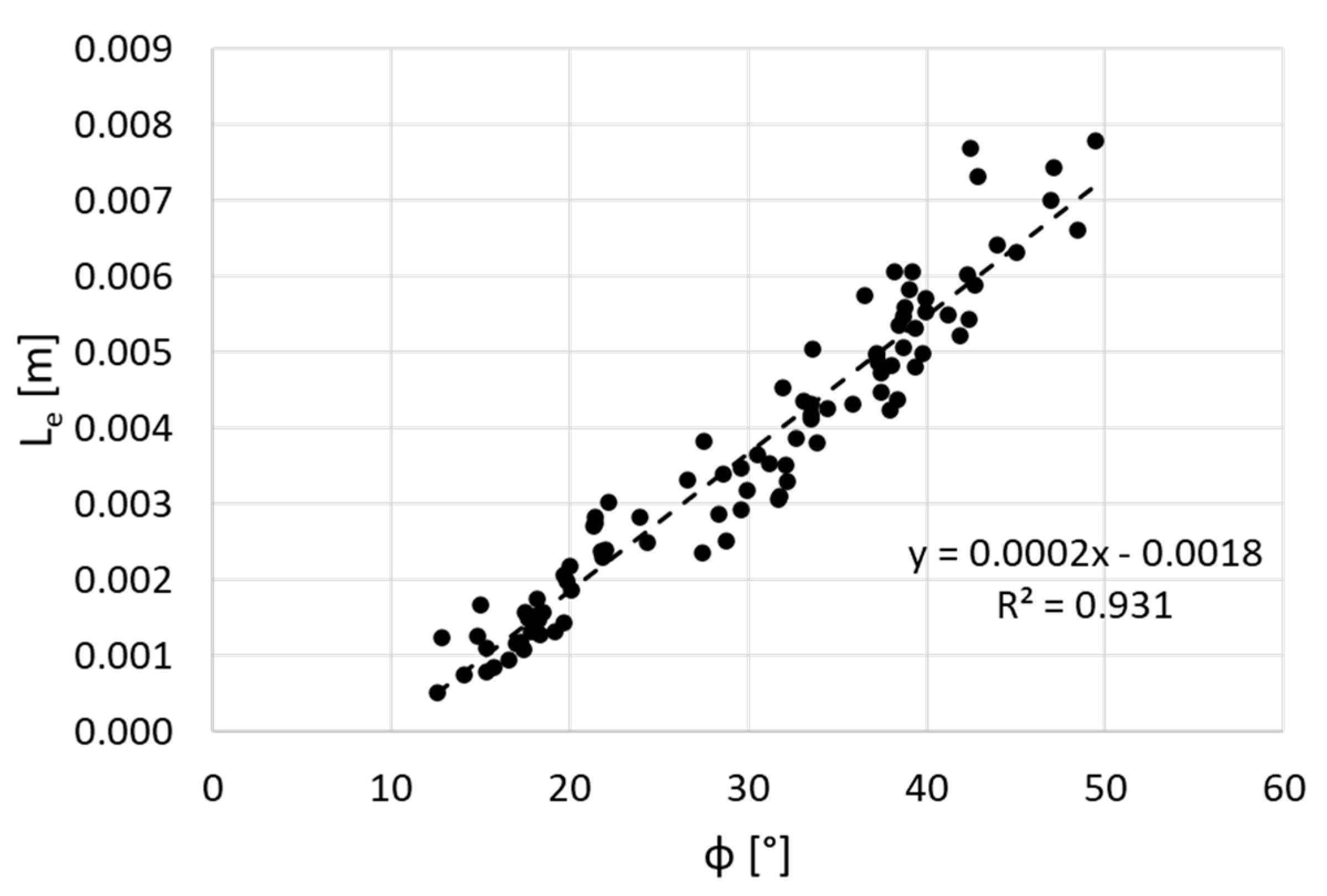
The prediction of L by using φ resulted in an average absolute error of 0.004 ± 0.002 m (8%). Figure 6 shows the behavior of this error as a function of φ.

According to van Dieen’s model, the variation of L with TP averages 0.001 m (Figure 1a). Since an error of 0.004 m is higher than this variation and by considering the linear behavior of L_e as a function of φ (r² = 0.931), L_φ was adjusted as follows:

$${\mathrm{L}}_{\mathsf{\phi }}^{\prime }={\mathrm{L}}_{\mathsf{\phi }}-\left(0.0002·\mathsf{\phi }\right)-0.0018$$

(8)

where 0.0002 and 0.0018 are the coefficients of the linear model shown in Figure 6.

When this correction was applied, L_e decreased to 0.001 ± 0.001 m. Person’s correlation analysis confirmed a strong association between L_TP and L_φ’ (r = 0.965, p < 0.0001), while Bland–Altman plot analysis revealed a high agreement between methods with a bias <0.001 m, upper and lower limits of agreement (uLOA) of 0.002 m and a lower limit of agreement (lLOA) < 0.001 m (Figure 7a).

Finally, the prediction of δ by using φ resulted in an average absolute error of 2.7° ± 1.3° (2%), which corresponds, approximately, to the variation of δ with TP according to van Dieen’s model (Figure 1b). For this reason, no correction was considered as needed for δ_φ. A strong correlation (r = 0.970, p < 0.0001) as well as high agreement (bias = 2.8°, uLOA = 5.3° and lLOA = 0.2°) were found between δ_TP and δ_φ (Figure 7b).

4. Discussion

The present technical note aimed at enriching the planar linked segment model originally proposed by Chaffin with the prediction of the moment arm and of the orientation of the line of action of the back extensor muscles during symmetric lifting tasks (stoop and squat techniques). Prediction equations were borrowed from the single equivalent muscle model proposed by van Dieen and de Looze [15]. Originally, these equations were meant to be fed with the sagittal plane component of the Euler rotation of a 3D thorax-embedded anatomical frame with respect to a 3D pelvis-embedded anatomical frame. In order to make these prediction equations compliant with a two-dimensional analysis, the angle formed by the segment joining L5/S1 to the shoulder joint centers with the longitudinal axis of the pelvis was introduced. To this end, the positions of the ASIS and PSIS were added to the original marker set (Figure 8).

In turn, the original set of anatomical landmarks proposed by Chaffin for his linked segment model was deprived of the hip joint center, as this point can predicted using ASIS and PSIS. The position of the shoulder joint center was also enhanced, as it was no longer assumed to coincide with the acromion. The model proposed by van Dieen and de Looze was validated within the angular range of 5° of trunk extension to 55° of trunk flexion, and the thorax-to-pelvis flexion angles computed from the available dataset fall within this range. The planar trunk flexion angle proposed in the present paper has proved to be highly correlated with the thorax-to-pelvis flexion angle used by van Dieen and de Looze (r = 0.970). The prediction equations proposed by van Dieen and de Looze were, hence, applied by using the newly computed planar trunk flexion angle regardless of its accuracy with respect to the thorax-to-pelvis flexion angle used by van Dieen and de Looze. A strong association (r = 0.970) and a high level of agreement (bias = 2.8°, upper limit of agreement = 5.3° and lower limit of agreement = 0.2°) was found between the orientation of the back extensor muscle line of action as predicted using the planar trunk flexion angle proposed in the present paper and the thorax-to-pelvis flexion angle used by van Dieen and de Looze. In their single muscle equivalent model, the orientation of the back extensor muscle line of action ranges from 100° to 134° with variations of 2.6°. This means that the average absolute error of 2.7° found between the two methods falls within the sensitivity of the prediction. On the other hand, the prediction of the moment arm of back extensor muscles by using the planar trunk flexion angle proposed in the present paper required a correction in order to achieve a sufficient accuracy with respect to the model proposed by van Dieen and de Looze. Since the prediction error showed a linear trend with respect to the planar angle used as input to the model, the error was subtracted through a linear regression model built with this set of data. As such, a strong association (r = 0.965) and a high level of agreement (bias <0.001 m, upper limit of agreement = 0.002 m and lower limit of agreement <0.001 m) were, hence, found between the moment arm of the back extensor muscles as predicted using the planar trunk flexion angle proposed in the present paper and the thorax-to-pelvis flexion angle used by van Dieen and de Looze. Since the average variation of the moment arm predicted by the model of van Dieen and de Looze during the considered range of trunk flexion is 0.001 m, the average absolute error of 0.001 m found between the two methods falls within the sensitivity of the prediction.

5. Conclusions

To conclude, the method proposed in the present paper allows one to use a bidimensional analysis performed on a video-taped image to estimate shear and compression forces by taking into account a variable back extensor muscle moment arm and line of action. The positions of seven palpable anatomical landmarks are needed from a video-taped image for model implementation. In particular, the proposed model leads to the estimation of a thorax-to-pelvis flexion angle from the planar positions of an augmented Chaffin’s marker set (Equation (5)). This angle is then used to feed van Dieen and de Looze regression equations to predict a trunk flexion-specific moment arm (Equation (6)) as well as a trunk-flexion specific line of action orientation (Equation (7)) to increase the accuracy in computing the contribution of the back extensor muscle force to the compression and shear forces acting on the L5/S1 intervertebral disc. An additional equation is presented to correct the error in predicting the back extensor muscle moment arm according to the planar trunk flexion angle proposed in the present paper (Equation (8)). The method proposed in the present paper was validated at a single instant of time, assuming it was a static trial, but the same can be applied during a dynamic task at each sampled moment in time. The analysis should be limited to symmetric lifting tasks only.

References

1. Cole, M.H.; Grimshaw, P.N. Low back pain and lifting: A review of epidemiology and aetiology. Work 2003, 21, 173–184. [Google Scholar] [PubMed]
2. Coenen, P.; Gouttebarge, V.; Van Der Burght, A.S.A.M.; Van Dieën, J.H.; Frings-Dresen, M.H.W.; Van Der Beek, A.J.; Burdorf, A. The effect of lifting during work on low back pain: A health impact assessment based on a meta-analysis. Occup. Environ. Med. 2014, 71, 871–877. [Google Scholar] [CrossRef] [PubMed] [Green Version]
3. Chaffin, D.B. A computerized biomechanical model-Development of and use in studying gross body actions. J. Biomech. 1969, 2, 429–441. [Google Scholar] [CrossRef] [Green Version]
4. Anderson, C.K.; Chaffin, D.B.; Herrin, G.D. A study of lumbosacral orientation under varied static loads. Spine 1986, 11, 456–462. [Google Scholar] [CrossRef] [PubMed]
5. Morris, J.M.; Lucas, D.B.; Bresler, B. Role of the Trunk in Stability of the Spine. J. Bone Jt. Surg. 1961, 43, 327–351. [Google Scholar] [CrossRef]
6. Daggfeldt, K.; Thorstensson, A. The mechanics of back-extensor torque production about the lumbar spine. J. Biomech. 2003, 36, 815–825. [Google Scholar] [CrossRef]
7. Chaffin, D.B.; Andersson, G.B.J.; Martin, B.J. Occupational Biomechanics, 4th ed.; John Wiley & Sons: Hoboken, NJ, USA, 2006; ISBN 978-0-471-72343-1. [Google Scholar]
8. Fischer, S.L.; Albert, W.J.; McClellan, A.J.; Callaghan, J.P. Methodological considerations for the calculation of cumulative compression exposure of the lumbar spine: A sensitivity analysis on joint model and time standardization approaches. Ergonomics 2007, 50, 1365–1376. [Google Scholar] [CrossRef] [PubMed]
9. Dreischarf, M.; Shirazi-Adl, A.; Arjmand, N.; Rohlmann, A.; Schmidt, H. Estimation of loads on human lumbar spine: A review of in vivo and computational model studies. J. Biomech. 2016, 49, 833–845. [Google Scholar] [CrossRef]
10. Malakoutian, M.; Street, J.; Wilke, H.J.; Stavness, I.; Fels, S.; Oxland, T. A musculoskeletal model of the lumbar spine using ArtiSynth–development and validation. Comput. Methods Biomech. Biomed. Eng. Imaging Vis. 2018, 6, 483–490. [Google Scholar] [CrossRef]
11. Robertson, D.G.E.; Caldwell, G.E.; Hamill, J.; Kamen, G.; Whittlesey, S.N. Research Methods in Biomechanics; Human Kinetics: Champaign, IL, USA, 2014. [Google Scholar]
12. Eskandari, A.H.; Arjmand, N.; Shirazi-Adl, A.; Farahmand, F. Subject-specific 2D/3D image registration and kinematics-driven musculoskeletal model of the spine. J. Biomech. 2017, 57, 18–26. [Google Scholar] [CrossRef]
13. Waters, T.R.; Lu, M.L.; Werren, D.; Piacitelli, L. Human posture simulation to assess cumulative spinal load due to manual lifting. Part I: Methods. Theor. Issues Ergon. Sci. 2011, 12, 176–188. [Google Scholar] [CrossRef]
14. Rajaee, M.A.; Arjmand, N.; Shirazi-Adl, A.; Plamondon, A.; Schmidt, H. Comparative evaluation of six quantitative lifting tools to estimate spine loads during static activities. Appl. Ergon. 2015, 48, 22–32. [Google Scholar] [CrossRef] [PubMed]
15. Van Dieën, J.H.; De Looze, M.P. Sensitivity of single-equivalent trunk extensor muscle models to anatomical and functional assumptions. J. Biomech. 1999, 32, 195–198. [Google Scholar] [CrossRef]
16. Van Dieën, J.H.; Van Der Burg, P.; Raaijmakers, T.A.J.; Toussaint, H.M. Effects of repetitive lifting on kinematics: Inadequate anticipatory control or adaptive changes? J. Mot. Behav. 1998, 30, 20–32. [Google Scholar] [CrossRef] [PubMed] [Green Version]
17. McConville, J.T.; Churchill, T.; Kaleps, I.; Clauser, C.E.; Cuzzi, J. Anthropometric Relationships of Body and Body Segment Moments of Inertia; Wright Patterson Air Force Base: Dayton, OH, USA, 1980. [Google Scholar]
18. Rab, G.; Petuskey, K.; Bagley, A. A method for determination of upper extremity kinematics. Gait Posture 2002, 15, 113–119. [Google Scholar] [CrossRef]
19. Harrington, M.E.; Zavatsky, A.B.; Lawson, S.E.M.; Yuan, Z.; Theologis, T.N. Prediction of the hip joint centre in adults, children, and patients with cerebral palsy based on magnetic resonance imaging. J. Biomech. 2007, 40, 595–602. [Google Scholar] [CrossRef] [PubMed]
20. Fiorentino, N.M.; Kutschke, M.J.; Atkins, P.R.; Foreman, K.B.; Kapron, A.L.; Anderson, A.E. Accuracy of Functional and Predictive Methods to Calculate the Hip Joint Center in Young Non-pathologic Asymptomatic Adults with Dual Fluoroscopy as a Reference Standard. Ann. Biomed. Eng. 2016, 44, 2168–2180. [Google Scholar] [CrossRef] [Green Version]
21. Bell, A.L.; Brand, R.A.; Pedersen, D.R. Prediction of hip joint centre location from external landmarks. Hum. Mov. Sci. 1989, 8, 3–16. [Google Scholar] [CrossRef]
22. Freivalds, A.; Chaffin, D.B.; Garg, A.; Lee, K.S. A dynamic biomechanical evaluation of lifting maximum acceptable loads. J. Biomech. 1984, 17, 251–262. [Google Scholar] [CrossRef] [Green Version]
23. Maurice, P.; Malaisé, A.; Amiot, C.; Paris, N.; Richard, G.L.; Rochel, O.; Ivaldi, S. Human movement and ergonomics: An industry-oriented dataset for collaborative robotics. Int. J. Rob. Res. 2019, 38, 1529–1537. [Google Scholar] [CrossRef] [Green Version]
24. Brehm, M.A.; Scholtes, V.A.; Dallmeijer, A.J.; Twisk, J.W.; Harlaar, J. The importance of addressing heteroscedasticity in the reliability analysis of ratio-scaled variables: An example based on walking energy-cost measurements. Dev. Med. Child Neurol. 2012, 54, 267–273. [Google Scholar] [CrossRef]
Figure 1. Variation of the back extensor muscle moment arm (a) and of the orientation of the line of action with respect to the plane of L5/S1 (b) from 0° to 55° of trunk flexion according to van Dieen’s single-equivalent muscle (SEM) model.
Applsci 10 06700 g001
Figure 2. The angle φ is supposed to be linearly related to the thorax-to-pelvis angle used by van Dieen to predict the back extensor muscle moment arm and line of action. The position of the origin of the pelvis-embedded anatomical reference frame, whose axes are depicted as dotted lines, is placed for graphical convenience to highlight the angle that the segment joining L5/S1 to S forms with the longitudinal axis of the pelvis-embedded anatomical reference frame. K = knee joint center; H = hip joint center; L5/S1 = intervertebral disc joint center; S = shoulder joint center; ASIS: anterior superior iliac spine; PSIS: posterior superior iliac spine
Applsci 10 06700 g002
Figure 3. Chaffin’s linked segment model (LSM) (upper arm and forearm are excluded) used to estimate the position of the L5/S1 (O) joint center. A = ankle joint center; K = knee joint center; H = hip joint center; S = shoulder joint center; γ = pelvic rotation angle; β = angle formed by the segment joining H to O with the horizontal axis; α = inclination of the trunk with respect to the horizontal axis; θ = inclination of the thigh with respect to the horizontal axis.
Applsci 10 06700 g003
Figure 4. Bland–Altman plot for visually inspecting the presence of heteroscedasticity (i.e., linear trend) in the dataset. The plot depicts the differences (error) between the angle of the thorax relative to the pelvis (TP) and φ against the respective means.
Applsci 10 06700 g004
Figure 5. Linear trend of φ with respect to TP depicting the strong association between these two variables.
Applsci 10 06700 g005
Figure 6. Linear trend of the error in predicting the back extensor muscle moment arm by using φ with respect to the degree of trunk flexion (φ).
Applsci 10 06700 g006
Figure 7. Bland–Altman plot analysis for repeated measurements depicting the absolute agreement between the back extensor muscle moment arm (a) and line of action (b) as predicted using TP and φ. Horizontal lines represent the bias (solid) and upper and lower limits of agreement (dotted). SD = standard deviation.
Applsci 10 06700 g007
Figure 8. Palpable anatomical landmarks required to use the planar linked segment model proposed by Chaffin enriched with the estimation of the back extensor muscle moment arm and line of action as suggested in the present paper. W = wrist joint center; E = elbow joint center; AC = acromion; PSIS = posterior superior iliac spine; ASIS = anterior superior iliac spine; K = knee joint center; A = ankle joint center.
Applsci 10 06700 g008