Ultrasonic Deicing Efficiency Prediction and Validation for a Flat Deicing System

Abstract

An effective deicing system is needed to be designed to conveniently remove ice from the surfaces of structures. In this paper, an ultrasonic deicing system for different configurations was estimated and verified based on finite element simulations. The research focused on deicing efficiency factor (DEF) discussions, prediction, and validations. Firstly, seven different configurations of Lead zirconate titanate (PZT) disk actuators with the same volume but different radius and thickness were adopted to conduct harmonic analysis. The effects of PZT shape on shear stresses and optimal frequencies were obtained. Simultaneously, the average shear stresses at the ice/substrate interface and total energy density needed for deicing were calculated. Then, a coefficient named deicing efficiency factor (DEF) was proposed to estimate deicing efficiency. Based on these results, the optimized configuration and deicing frequency are given. Furthermore, four different icing cases for the optimize configuration were studied to further verify the rationality of DEF. The effects of shear stress distributions on deicing efficiency were also analyzed. At same time, a cohesive zone model (CZM) was introduced to describe interface behavior of the plate and ice layer. Standard-explicit co-simulation was utilized to model the wave propagation and ice layer delamination process. Finally, the deicing experiments were carried out to validate the feasibility and correctness of the deicing system.

1. Introduction

Icing on the equipment is one of the problems needed to be solved in a cold region. Ice buildup on the structures may cause many adverse effects, including cracking, stiffness degradation, malfunctions, and low performance on the structural components, which remarkably endangers their reliability. Icing problems are widely existing in aircraft [1,2], wind turbine blades [3,4], marine structures [5,6] etc. So far, various deicing methods were proposed and developed, mainly including hot bleed air, electro-thermal, electro-impulse, electro-expulsive, vibratory, high frequency microwave, deicing fluids etc. [7,8,9]. Based on the theory of wave propagation in a multilayered structure, Lamb waves and shear horizontal (SH) waves can generate stress and displacement at the interface of the structure. These stresses can be utilized to detach the ice layer. Compared to the deicing techniques mentioned above, ultrasonic deicing is more advantageous in terms of power consumption and efficiency. Meanwhile, the damping coefficient of the Lamb wave is small and this property guarantees the long propagation distance of the Lamb wave. Thus, the Lamb wave has an advantage in deicing for large structures.

Many scholars have done a lot of meaningful work on ultrasonic deicing before. The preliminary research mainly focused on the feasibility study of ultrasonic deicing. Ramanathan [10] studied the use of shear horizontal waves to provoke ice delamination by exceeding the ice adhesion strength by Lead zirconate titanate (PZT) actuator, which showed very promising results. JL Palacios et al. [11] focused on researching the deicing system for helicopter blades based on ultrasonic shear vibration and impedance matching for the system. Ultrasonic vibration to remove ice from pipes was investigated by RA Seppings [12]. Congbo Yin et al. [13] validated the feasibility of ultrasonic deicing for the wind turbine blade. Marc Budinger et al. [14] investigated electromechanical deicing system based on piezoelectric actuators and resonance modes. MK Kalkowski et al. [15] analyzed structures with unwanted accretions based on semi-analytical finite elements to detach unwanted build-up. A thorough parametric study of the ultrasonic deicing method on a plate with coating was conducted by Shi et al. [16]. Some research focused on improving deicing efficiency. Tailored waveguides (TWG) were introduced to reduce power required for deicing by Zhu [17]. Nicola DiPlacido et al. [18] compared the effects of two actuation methods for piezoelectric actuators on deicing. The results indicated, for equal input power, the multitransient actuation method would increase deicing stresses compared to continuous excitation. Wang et al. [19] designed a light piezoelectric transducer for deicing. The deicing efficiency was also explored based on theory. The interface shear concentration coefficient (ISCC) derived from the theory of waves propagation in structure was defined and explored to guide for deicing [16,20,21]. This coefficient considered the thickness of each layer but assumed the length and width of each layer was infinite. The reflection, superposition, mode conversion of waves, and actual boundary conditions are not considered. Electric power needed for deicing was another indicator used widely in Refs [11,22] to estimate deicing efficiency. However, the prerequisite for comparing power is the same deicing effect. In many cases, both the deicing power and deicing effect are different. Thus, it is necessary to explore a method to estimate deicing efficiency for an actual structure and different configuration.

For the ultrasonic deicing system, deicing energy and efficiency are two critical issues during the deicing process. In this paper, deicing energy was estimated from the perspective of conservation of energy and deicing efficiency for different models was investigated, which can provide guidance for deicing model selection to achieve deicing with reduced energy consumption. With help of numerical simulations, deicing efficiency for a flat deicing system can be revealed and predicted to optimize the deicing system. In the process, harmonic analysis coupled electrical and mechanical responses for the piezoelectric deicing system was performed to simulate steady-state ultrasonic vibration. Shear stresses at the interface of the ice layer were calculated and presented. The geometry effects of piezoelectric actuators on shear stress and power consuming were investigated. Based on that, the deicing efficiency factor (DEF) was proposed to describe deicing efficiency for seven different configurations, which is very meaningful for deicing result evaluations. Then, four icing cases were studied to validate DEF. Meanwhile, the shear stress distributions along three different axis directions were discussed. Based on results of harmonic analysis, a cohesive zone model (CZM) [23,24] was introduced in the standard-explicit co-simulation [25,26] process to study the wave propagation and deicing process. Finally, according to parameters used in finite element simulations, the experiment platform was founded and deicing experiments were conducted to verify the feasibility of the system.

2. Basic Theory and Model Establishment

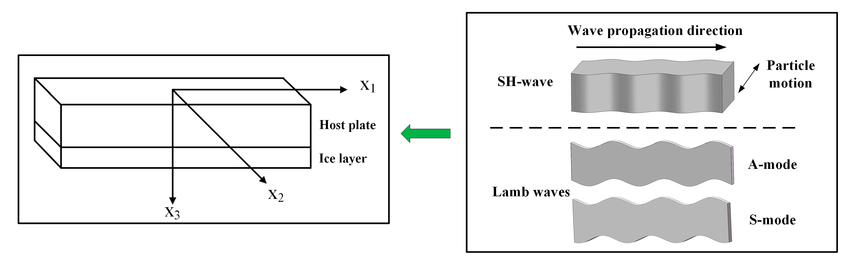
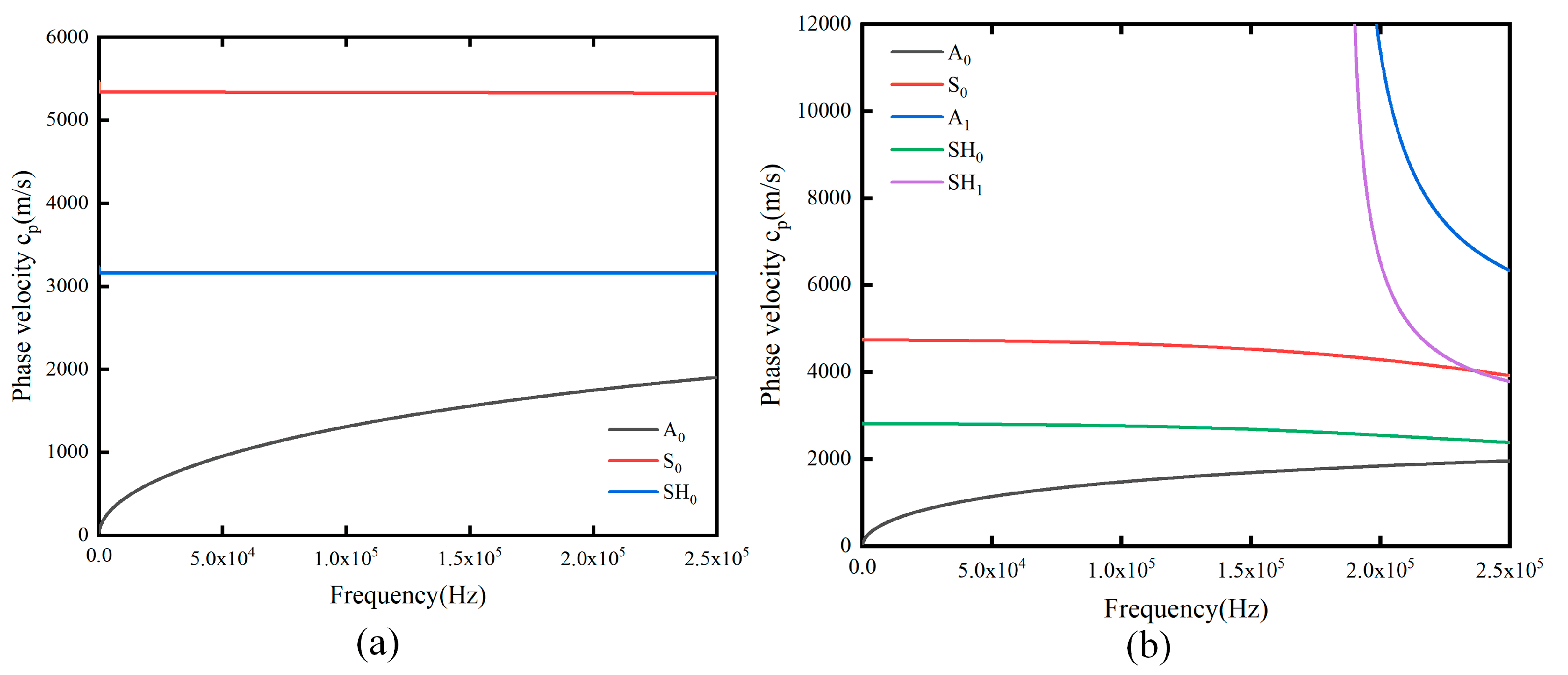
2.1. Ultrasonic Deicing Principle Interpretation

After the actuator bonded to the flat deicing system is turned on, Lamb waves and shear horizontal (SH) waves are generated in the structure. When the shear stress caused by these two kinds of waves exceed the ice adhesion strength, the ice layer is detached from the plate. The waves propagation in multiple layers of isotropic solid media can be investigated based on theory in Ref [27]. The coordinate system and ultrasonic waves propagating in the ice-plate layered structure for deicing is shown in Figure 1.

The governing equation for Lamb waves and SH waves can be written as:

$$\rho \frac{{\partial }^2{u}_i}{\partial t^2}=c_{ijkl}\frac{{\partial }^2{u}_i}{\partial x_j\partial x_k},$$

(1)

where ρ is the density, C_ijkl is the stiffness tensor, and u_i is the displacement field. The waves are assumed to propagate along x₁ direction. The solution of Equation (1) can be assumed as the following form:

$$u_i=U_i{\mathrm{e}}^{ik(x_1+\alpha x_3-ct)}.$$

(2)

In Equation (2), U_i = Uα_i, α_i is the cosine component in i direction. U_i is the polarization vector presenting the displacement in each direction, k stands for the wave number along x₁ direction, c represents the phase velocity along x₁ direction, and α is the ratio of wave number in x₃ with respect to the wave number in the x₁ direction. By utilizing the inverse method [28], Christoffel’s equation can be written as Equation (3):

$$\left[\begin{array}{ccc}{\lambda }_{11}-\rho c^2& {\lambda }_{12}& {\lambda }_{13}\\ {\lambda }_{12}& {\lambda }_{22}-\rho c^2& {\lambda }_{23}\\ {\lambda }_{13}& {\lambda }_{23}& {\lambda }_{33}-\rho c^2\end{array}\right]\left\{\begin{array}{c}{U}_1\\ U_2\\ U_3\end{array}\right\}=\left\{\begin{array}{c}0\\ 0\\ 0\end{array}\right\}.$$

(3)

The values of λ_im (i, m = 1, 2, 3) in Equation (3) can be calculated from Equation (4):

$${\lambda }_{\mathrm{im}}=C_{iklm}{n}_k{n}_l,$$

(4)

where n_k, n_l are the direction cosines of the normal to the wave front. According to the boundary conditions, the displacements u₁ and u₃ are zero for SH waves and u₂ is zero for Lamb waves. Thus, displacements and stresses can be expressed as Equation (5):

$$u_1={\displaystyle \sum _{k=1}^4{B}_k{\mathrm{e}}^{ik(x_1+{\alpha }_k{x}_3-ct)}}$$

$$u_2={\displaystyle \sum _{k=1}^2{B}_k{\mathrm{e}}^{ik(x_1+{\alpha }_k{x}_3-ct)}}$$

$$u_3={\displaystyle \sum _{k=1}^4{B}_k{U}_{3k}{e}^{ik(x_1+{\alpha }_k{x}_3-ct)}}$$

$${\sigma }_{31}={\displaystyle \sum _{k=1}^4{B}_k\left[{\alpha }_k+U_{3k}\right]\mu \left(ik\right)e^{ik(x_1+{\alpha }_k{x}_3-ct)}}$$

$${\sigma }_{32}={\displaystyle \sum _{k=1}^2{B}_k{\alpha }_k\mu \left(ik\right){\mathrm{e}}^{ik(x_1+{\alpha }_k{x}_3-ct)}}$$

$${\sigma }_{33}={\displaystyle \sum _{k=1}^4{B}_k\left[\lambda +\left(\lambda +2\mu \right){\alpha }_k{U}_{3k}\right]\left(ik\right){\mathrm{e}}^{ik(x_1+{\alpha }_k{x}_3-ct)}},$$

(5)

where B_k is the weighting coefficient of the partial waves. U_3k is the relation of the polarization vectors between U₃ and U₁. The other variables are the same as mentioned before.

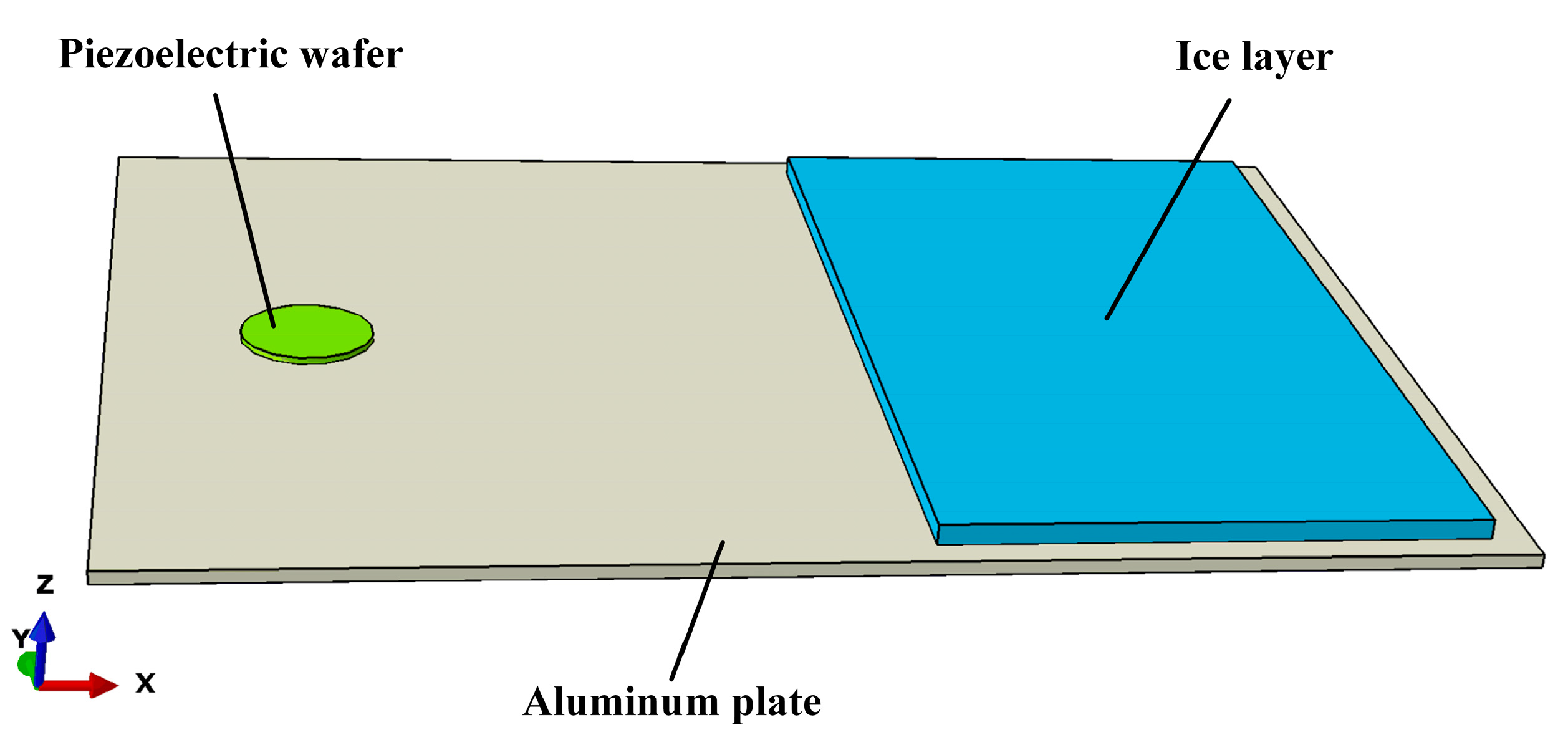
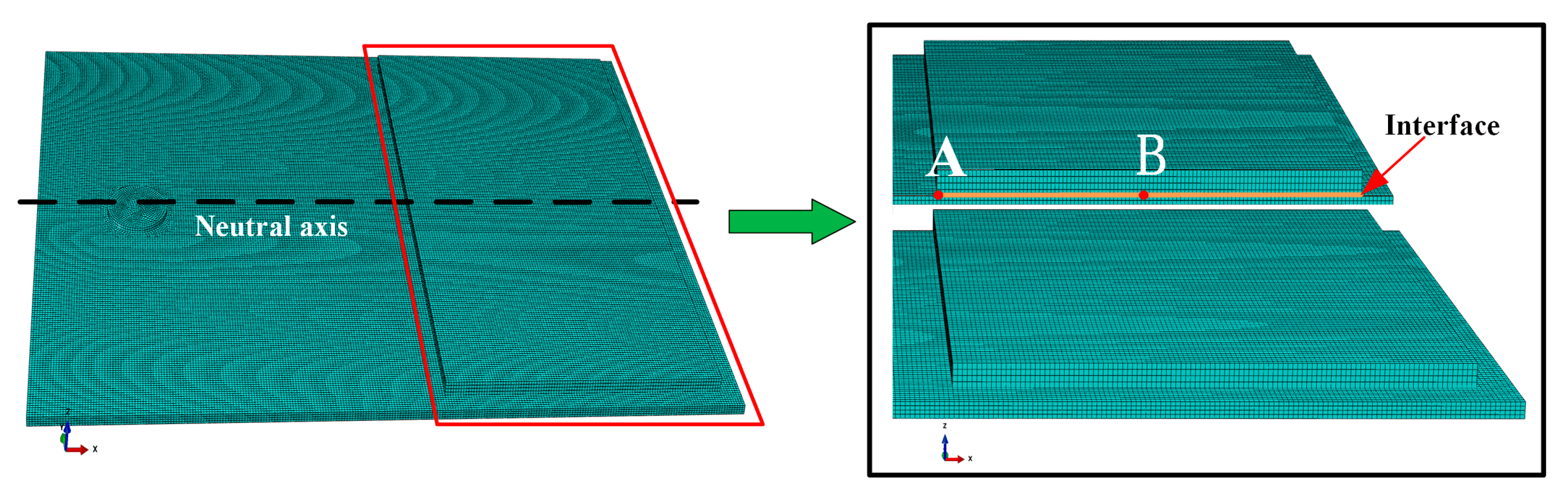
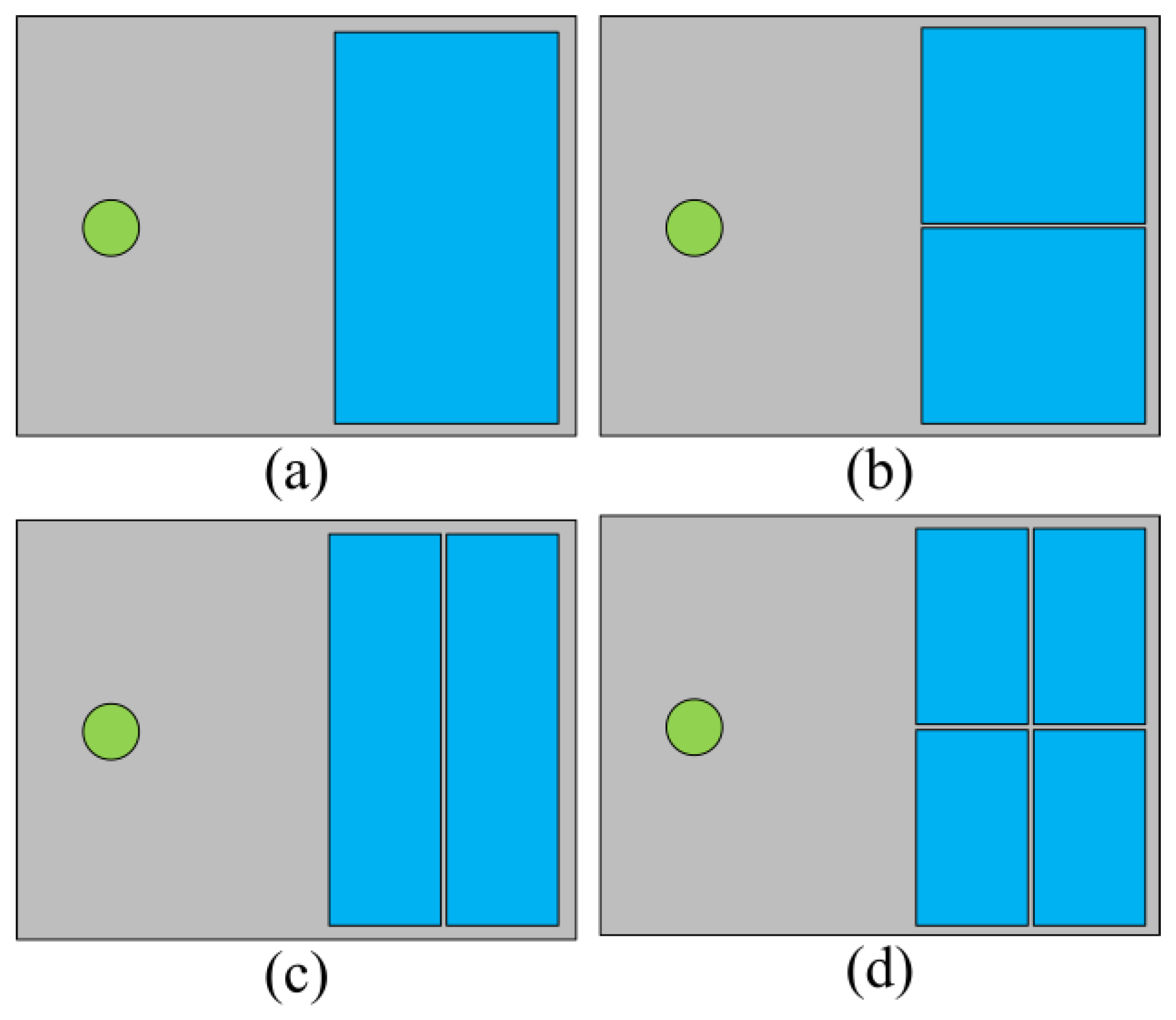
2.2. FE Model and Simulation

In this section, harmonic analysis and dynamic analysis were performed to model deicing effect and deicing process, respectively. Harmonic analysis was implemented to calculate the stress tensor at expected frequency range. The finite element model equation of the PZT actuator bonded to the host structure can be written as Equation (6) [29]:

$$F=([K_{nn}-w^2[M]-jw[R])U+[K_{n\Phi }]\Phi \left(\frac{I}{jw}\right)=[K_{n\Phi }]U+[K_{\Phi \Phi }]\Phi ,$$

(6)

where F is applied mechanical force, I is excitation current, U is elastic displacement field, Φ is electric potential, [K_nn] is elastic rigidity matrix, [K_nΦ] is piezoelectric stiffness matrix, [K_ΦΦ] is permittivity matrix, [M] is mass matrix, [R] is dissipation matrix, and w is the angular frequency. The equation of harmonic analysis used in FE software can be expressed as follows:

$$\left[\begin{array}{cc}{K}_{nn}-w^{2}M& K_{n\Phi }\\ K_{n\Phi }& K_{\Phi \Phi }\end{array}\right]\left[\begin{array}{c}U\\ \Phi \end{array}\right]=\left[\begin{array}{c}0\\ -Q\end{array}\right].$$

(7)

The work started from the evaluation of the effectiveness of guided waves technology to produce the ice detaching from the structure. The 3D model of finite element simulation is shown in Figure 2.

The geometry size of the aluminum plate and ice layer was 200 mm × 150 mm × 2 mm and 140 mm × 80 mm × 3 mm. The material of the piezoelectric disc was selected to be PZT-4. The material properties of the aluminum and ice are shown in

Table 1. The material properties.

Material	Density (kg/m3)	Young’s Modulus (GPa)	Poisson’s Ratio
Ice	920	9	0.28
Aluminum	2700	70	0.30

.

Material properties for PZT-4 are shown as follows:

$$\rho {=7500\mathrm{kg}/\mathrm{m}}^3\hspace{1em}{c}^E=\left[\begin{array}{cccccc}13.9& 7.78& 7.43& & & \\ 7.78& 13.9& 7.43& & & \\ 7.43& 7.43& 11.5& & & \\ & & & 2.56& & \\ & & & & 2.56& \\ & & & & & 2.56\end{array}\right]\times {10}^{10}\mathrm{Pa}$$

$$e=\left[\begin{array}{ccc}0& 0& -5.2\\ 0& 0& -5.2\\ 0& 0& 15.1\\ 0& 12.7& 0\\ 12.7& 0& 0\\ 0& 0& 0\end{array}\right]{\mathrm{c}/\mathrm{m}}^2\hspace{1em}\epsilon =\left[\begin{array}{ccc}762.5& & \\ & 762.5& \\ & & 663.2\end{array}\right],$$

where $\rho$ is density, $c^E$ is elasticity matrix, $e$ is piezoelectric coupling constant, and $\epsilon$ is dielectric matrix. The FE simulations were performed with an Abaqus^® during processing. The host plate and ice layer were meshed by using 20-node quadratic brick elements with reduced integration (C3D20R) [30] and PZT actuator was meshed by using 20-node quadratic piezoelectric brick elements with reduced integration (C3D20RE). In the frequency range of research (20–240 kHz), the wavelengths of the Lamb wave and SH wave were taken into consideration. According to the theory of guided waves in layered structures in Ref. [27], the global matrix method can be used to solve the dispersion curves of the ice-plate layered structure when ice accretes on the plate. By solving dispersion curve equations for both Lamb wave and SH wave, the phase velocity of both Lamb wave and SH wave can be calculated. The results for the 2 mm aluminum plate and 2 mm aluminum plate with a 3 mm ice layer are shown in Figure 3.

According to phase velocity, the shortest wavelengths should be around 8.0 mm for the 2 mm aluminum plate with a 3 mm ice layer and around 7.8 mm for the 2 mm aluminum plate at frequency 240 kHz. After several times trial calculations, the global mesh seeding size was chosen as 0.74 mm, smaller than one over ten the smallest wavelength. Meanwhile, the mesh type adapted in simulations was 20-node quadratic brick elements with reduced integration, rather 8-node linear brick elements with reduced integration to ensure accuracy. Thus, the amount of calculation would be several times larger than using mesh type 8-node linear brick elements with reduced integration. After meshing the model, the number of elements was more than 310,000. The FE mesh and reference points (A and B) for FE study is shown in Figure 4. In the model, the voltage applied to the positive and negative electrode of the actuator was 25 and 0 V, respectively. The left and right edge of the aluminum plate were fixed. To make out the effect of different actuators on deicing and stress distributions, the volume of the PZT actuator was kept as 100 π mm³, while their radius (r) and thickness (t) were changing as seven different configurations. The radius for seven configurations were 4, 5, 6, 7, 8, 9, and 10 mm, respectively.

Then, the deicing efficiency factor (DEF) was defined. The deicing efficiency for these seven configurations were compared. Based on simulation results in Section 4, the most efficient configuration was confirmed to be configuration 2. To verify the rationality of DEF, four different icing cases as shown in Figure 5 were studied. For these four cases, the radius of the PZT actuator was 5 mm. The icing case (a) in Figure 5 was the same as configuration 2 mentioned above. The size of the icing area and the centroid of ice layer for these four cases were the same. For the cases (b–d) in Figure 5, the distance between each ice block was 4 mm. Meanwhile, the applied voltage and frequency were the same for these four cases. Based on these, shear stresses and DEF were computed and verified.

Finally, Abaqus standard-explicit co-simulation was conducted to model wave propagation and the deicing process for configuration 2. The aluminum plate and ice layer were defined as the parent model to conduct transient dynamic analysis in Abaqus explicit, while the PZT actuator was defined as the child model to conduct Abaqus implicit analysis. An interaction interface between the PZT actuator and aluminum plate was used to manage the data exchange between the two solvers. A bilinear cohesive zone model (CZM) [23] was considered to simulate delamination behavior at the interface of the ice layer and aluminum plate. Cohesive elements with zero thickness were inserted between the aluminum plate and ice layer. The constitutive behavior of the cohesive layer was defined as a traction-separation law to model the detachment at the interface of the ice layer and aluminum plate. It is assumed that there is a linear elastic traction separation law before failure, and the material stiffness will gradually degrade after failure. To describe cohesive material behavior, damage initiation and damage evolution should be defined. Initiation of interface damage is based on quadratic traction interaction failure criterion, written as Equation (8):

$$\begin{array}{l}\sqrt{{\left(\frac{{\sigma }_z}{T}\right)}^2+{\left(\frac{{\tau }_{xz}}{S}\right)}^2+{\left(\frac{{\tau }_{yz}}{S}\right)}^2}=1({\sigma }_z>0),\\ \sqrt{{\left(\frac{{\tau }_{xz}}{S}\right)}^2+{\left(\frac{{\tau }_{yz}}{S}\right)}^2}=1({\sigma }_z\le 0)\end{array}$$

(8)

where ${\sigma }_z$, ${\tau }_{xz}$, ${\tau }_{yz}$ represent the normal stress, shear stress in the x and y direction, separately. T and S are the tensile strength and shear strength, respectively. The damage evolution satisfies the mixed-mode fracture energy approach [31,32]. The fracture energy for the aluminum/ice interface was reported to be 1.0 N/m [33]. Therefore, the normal mode fracture energy G_IC was considered to be 1.0 × 10⁻³ N/mm in this study. The shear mode fracture energy G_IIC and G_IIIC was 2.0 × 10⁻³ N/mm. The failure criterion can be expressed as Equation (9):

$${\left(\frac{G_I}{G_{Ic}}\right)}^{\alpha }+{\left(\frac{G_{II}}{G_{IIc}}\right)}^{\alpha }+{\left(\frac{G_{III}}{G_{IIIc}}\right)}^{\alpha }=1,$$

(9)

where G_I, G_II, G_III are energy produced in the normal, the x and y direction, respectively. G_IC, G_{II C}, G_IIIC are the critical fracture energy to achieve debond failure in the normal, the x, and the y direction, respectively. The value of exponent α is usually 1 or 2. It was selected to be 2 in this study. The relevant parameters can refer to literatures reported before [31]. All parameters are summarized in

Table 2. Cohesive material properties.

Parameters	Values
Cohesive layer modulus (penalty stiffness) in all 3 directions, Knn, Kss, Ktt	1.0 × 106 N/mm3
Ultimate strength in tensile, T	0.8 MPa
Ultimate strength in mode II, S	0.8 MPa
Ultimate strength in mode III, N	0.8 MPa
Normal mode fracture, GIC	1.0 × 10−3 N/mm
Normal mode fracture, GIIC	2.0 × 10−3 N/mm
Normal mode fracture, GIIIC	2.0 × 10−3 N/mm

.

To obtain the convergent result of the explicit dynamic procedure, the element size and time step should be considered. The element size was the same as mention above (0.74 mm). According to Courant criteria and Nyquist criteria, the time step was sited to be 2 × 10⁻⁸ s. Time period was 6 × 10⁻⁴ s. The voltage applied the actuator was a sinusoidal load of 25 V. The other boundary condition was the same as mentioned in the harmonic analysis.

In order to solve such a huge amount of calculation, the supercomputer of National Supercomputer Center in Guangzhou, which is currently the fourth fastest supercomputer in the world, with a measured 33.86 petaflop/s (quadrillions of calculations per second), was used to perform these simulations. In these processes, we changed the number of nodes which is related to the number of CPUs used for computation, threads, and processes by running scripts to adjust the efficiency of parallel operation of supercomputer Tianhe-2. In this way, simulation results can be obtained most efficiently.

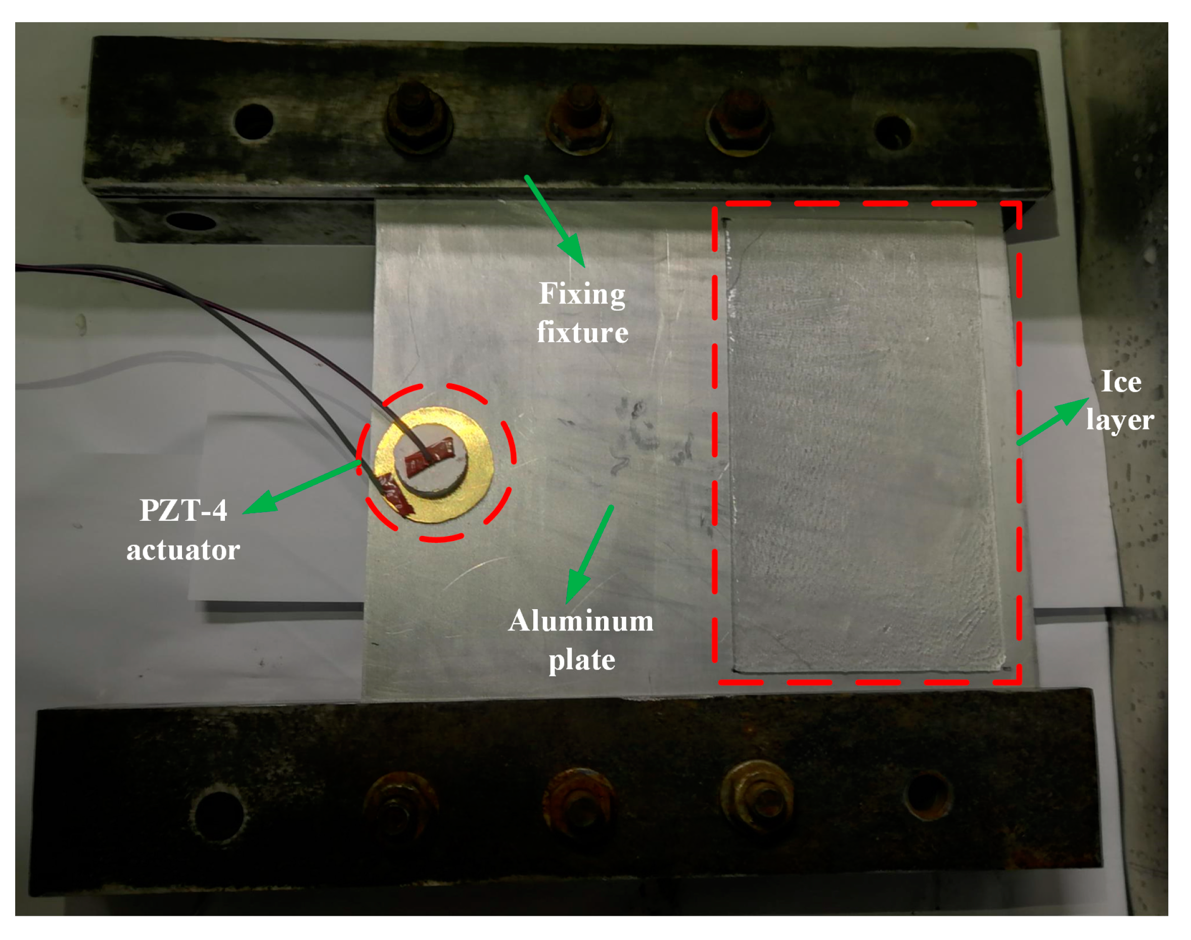
3. Deicing Experimental Setup and Schemes

On the basis of FE simulations, the experimental platform was built. In this part, the most efficient configuration 2 (according to simulation results in part 4) was mainly considered to validate the feasibility and rationality of the ultrasonic deicing system.

Ice adhesion strength varies from icing temperature, humid, surface roughness, measurement error etc. In this study, the ice adhesion strength was measured using a low temperature centrifuge, which is similar to these reported [16,34]. After completing all settings, the temperature of the low temperature centrifuge was turned to −12 °C for another 40 min and the centrifuge apparatus started. The rotate speed of the centrifuge was recorded when the ice layer was detached from the sample. In the calculation process, the centrifugal force was written as F = mrω². Then, ice adhesion strength can be calculated based on equation τ = F/A. F is centrifugal force (N), m is ice mass (0.00862 ± 0.0002 kg), r is radius of centrifuge apparatus (0.135 m), ω is speed of rotation (rad/s), τ is ice adhesion stress (Pa), A is icing area (0.00070686 m²). Ice adhesion strength was calculated to be 0.36 ± 0.06 MPa after 8 experiments.

All the settings were the same as mentioned in Section 2. In the experiment, a piezoelectric disk with radius 5 mm and thickness 4 mm was used as an actuator to generate ultrasonic waves. The piezoelectric disk was bonded to the aluminum plate by epoxy resin. The setup for the deicing experiments is shown in Figure 6. To eliminate the effect of surrounding temperature on the results, the whole experiment process was conducted in the refrigerator at −12 °C.

Three different frequencies 190, 213, and 236 kHz, respectively, were adopted to verify optimal frequency for configuration 2. These three frequencies were optimal frequencies for configuration 7 (r = 10 mm), configuration 2 (r = 5 mm), and configuration 3 (r = 6 mm), respectively. All the boundary conditions were the same for these three deicing experiments (including the size and location of ice layer), except the frequency applied to the PZT actuator. After 90 s testing for these three different frequencies, the final deicing effects can be obtained. Moreover, deicing experiments were also carried out for the remaining six groups to compare their differences of deicing effect and validate the correctness of simulation results. Finally, deicing experiments of four different icing cases for configuration 2 were carried out to verify the rationality of DEF.

4. Results and Discussion

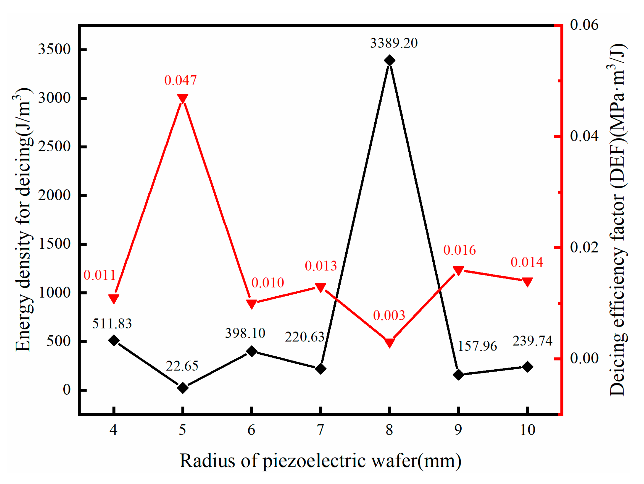
4.1. Deicing Energy Efficiency

After harmonic analysis, several nodes were selected as reference points to confirm optimal frequencies for each configuration. Due to the amount of data, only configuration 1 (r = 4 mm, t = 6.25 mm) was shown as an example to interpret the whole process. Here, only the two reference points A and B shown in Figure 4, which are located at the boundary and center of the interface between the host plate and ice layer, respectively, were presented as an example to output shear stress amplitude-frequency curves. The shear stress amplitude-frequency curves are shown in Figure 7. The optimal frequency results for the rest nodes were the same, so they were not presented here.

From the results of Figure 7, it can be found that the optimal frequency for deicing is 221 kHz. Then, the same processes were performed for the remaining six configurations to obtain the optimal frequency of each model. For the purpose of estimating the deicing effect of each model, the average shear stresses for delamination τ₁₃ and τ₂₃ at the interface of the ice layer were calculated. The results are shown in

Table 3. Optimal frequency and the average shear stresses at the interface for seven configurations.

Configuration Radius (mm)	Optimal Frequency (kHz)	τ13 (MPa)	τ23 (MPa)
4	221	4.33	3.01
5	213	0.64	0.85
6	236	2.99	2.75
7	222	1.92	2.02
8	232	7.22	6.94
9	212	1.75	1.77
10	190	2.27	2.42

.

From the results of Table 3, the total shear stress τ_total for delamination can be calculated from Formula (10):

$${\tau }_{\mathrm{total}}=\sqrt{{\tau }_{13}{}^2+{\tau }_{23}{}^2}.$$

(10)

The total shear stresses for seven different configurations are shown in Figure 8. These shear stresses were enough to overcome ice adhesion strength measured in lab condition, which was 0.36 ± 0.06 MPa at temperature −12 °C (detailed information is in part 3).

Besides deicing shear stresses analysis, energy consumed for the deicing system is another important aspect needed to take into consideration. For simplicity, the energy dissipation and heat loss were ignored, only the kinetic energy and strain energy for the whole system were considered to estimate the energy consumed for each model at optimal frequency. Therefore, the energy density for deicing can be written as Formula (11):

$$w=\frac{E_{\mathrm{k}}+U}{V},$$

(11)

where w, E_k, U, and V represent energy density, kinetic energy, strain energy, and volume of system, respectively, for deicing. From these data, the energy density needed to detach ice from the host plate for each model can be estimated. From computation results, the conclusion can be drawn that the energy density needed for deicing varies from the radius of the piezoelectric wafer with the system at optimal frequency for each configuration. Meanwhile, the deicing effect also differs from one to another. Therefore, it is difficult to distinguish which model is better. The ideal goal is to achieve deicing with minimum energy consumption. Therefore, a coefficient called deicing efficiency factor (DEF) was proposed to describe the relationship between deicing effect and deicing energy density. DEF was defined as Equation (12):

$$\mathrm{DEF}=\frac{{\tau }_{\mathrm{total}}}{w}=\frac{\sqrt{{\tau }_{13}{}^2+{\tau }_{23}{}^2}}{\frac{E_{\mathrm{k}}+U}{V}}=\frac{\sqrt{{\tau }_{13}{}^2+{\tau }_{23}{}^2}\cdot V}{E_{\mathrm{k}}+U},$$

(12)

where τ_total, τ₁₃, τ₂₃, w, E_k, U, and V have the same meaning as mentioned prior. This coefficient can describe deicing efficiency for each model. The greater this coefficient is, the greater total shear stress obtained at the same energy density, indicating that more energy is applied to detach ice, which represents the system as more efficient. From above data and Equation (12), DEF for each configuration can be calculated. The energy density needed for deicing and DEF of seven different configuration are shown in Figure 9. From these simulation results, it can be found that configuration 2 (r = 5 mm, t = 4 mm) is the most efficient one.

Then four icing cases based on configuration 2 mentioned in Section 2.2 were studied and compared. The shear stresses and DEF for these four cases were computed and shown in Figure 10. For these four icing cases, the deicing energy density was the same for the voltage and frequency applied to the PZT actuator. Therefore, the trend of DEF is consistent with that of the total shear stress for delamination (as shown in Figure 10b). Based on the simulation results, deicing experiments can be carried out to verify the rationality of DEF.

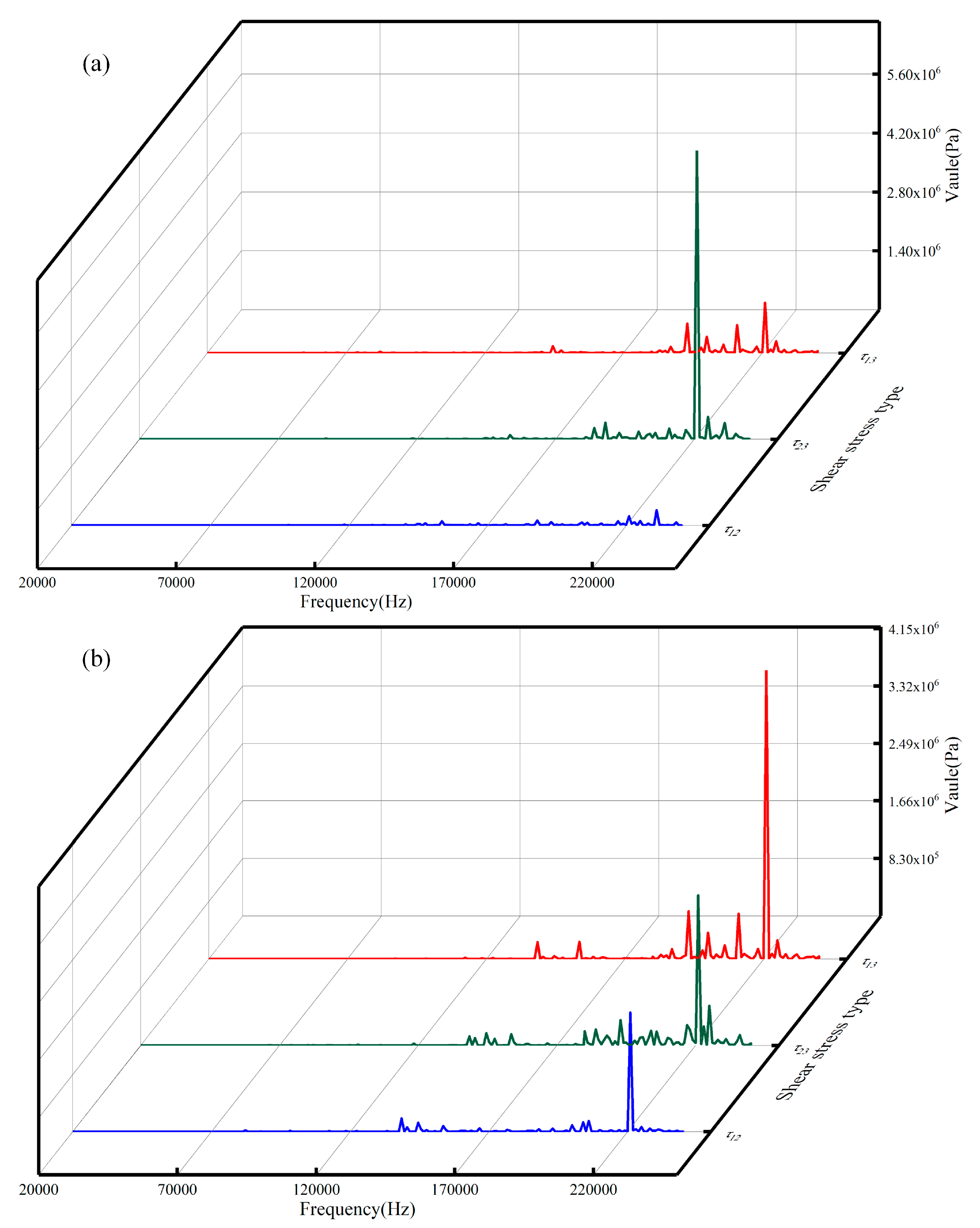
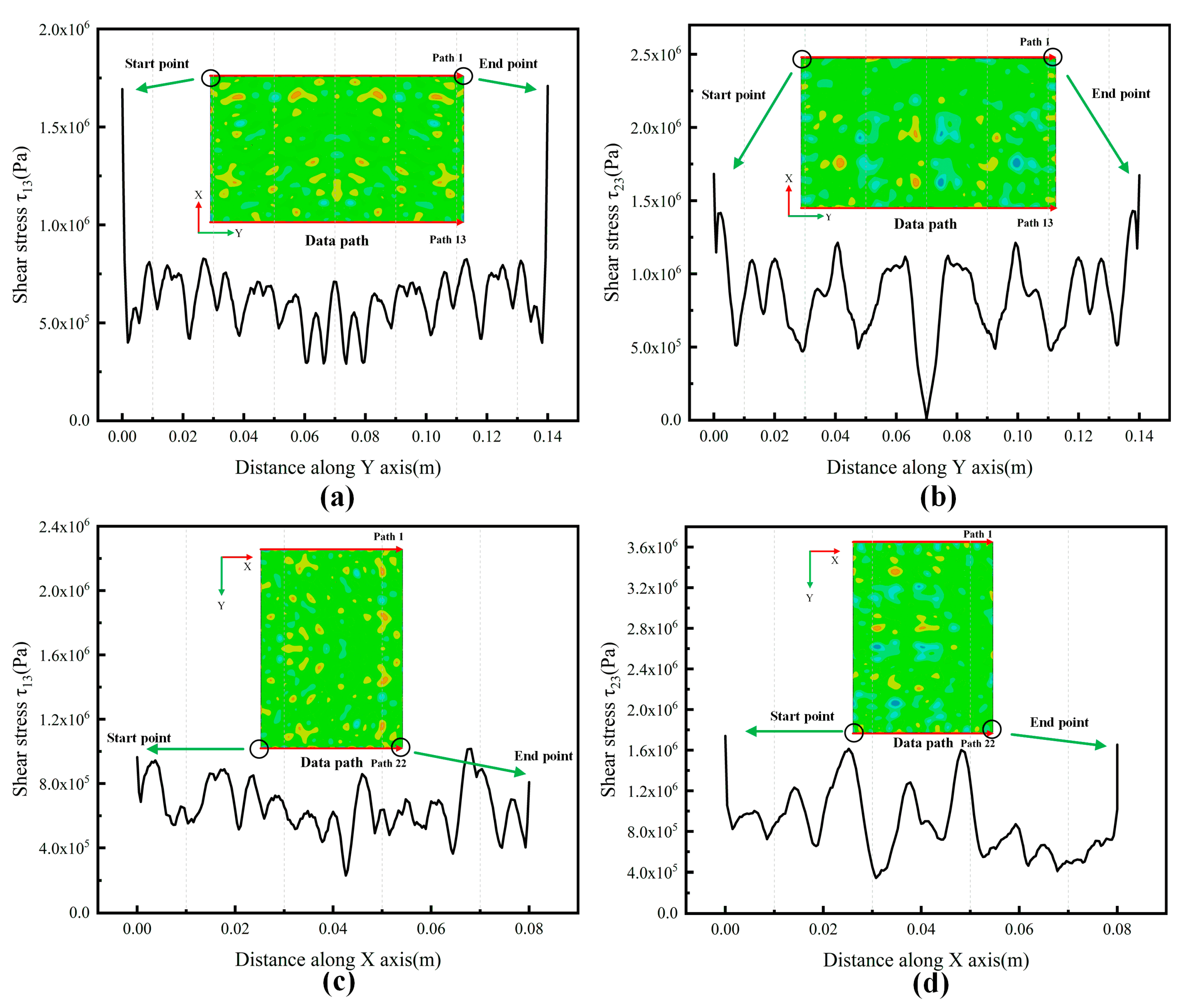
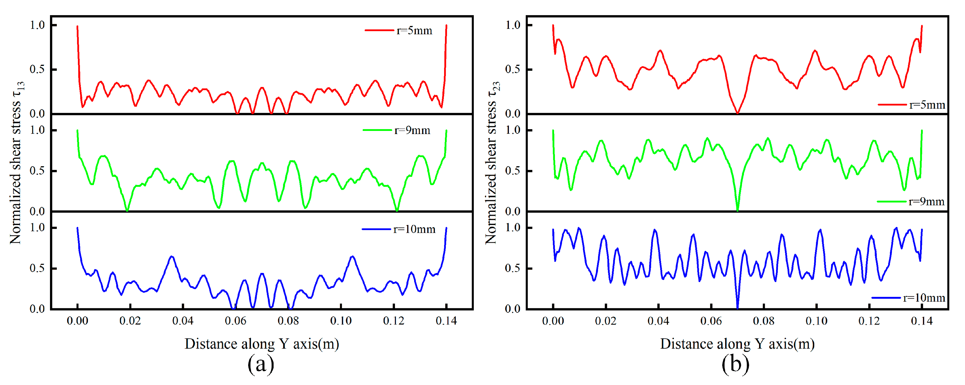
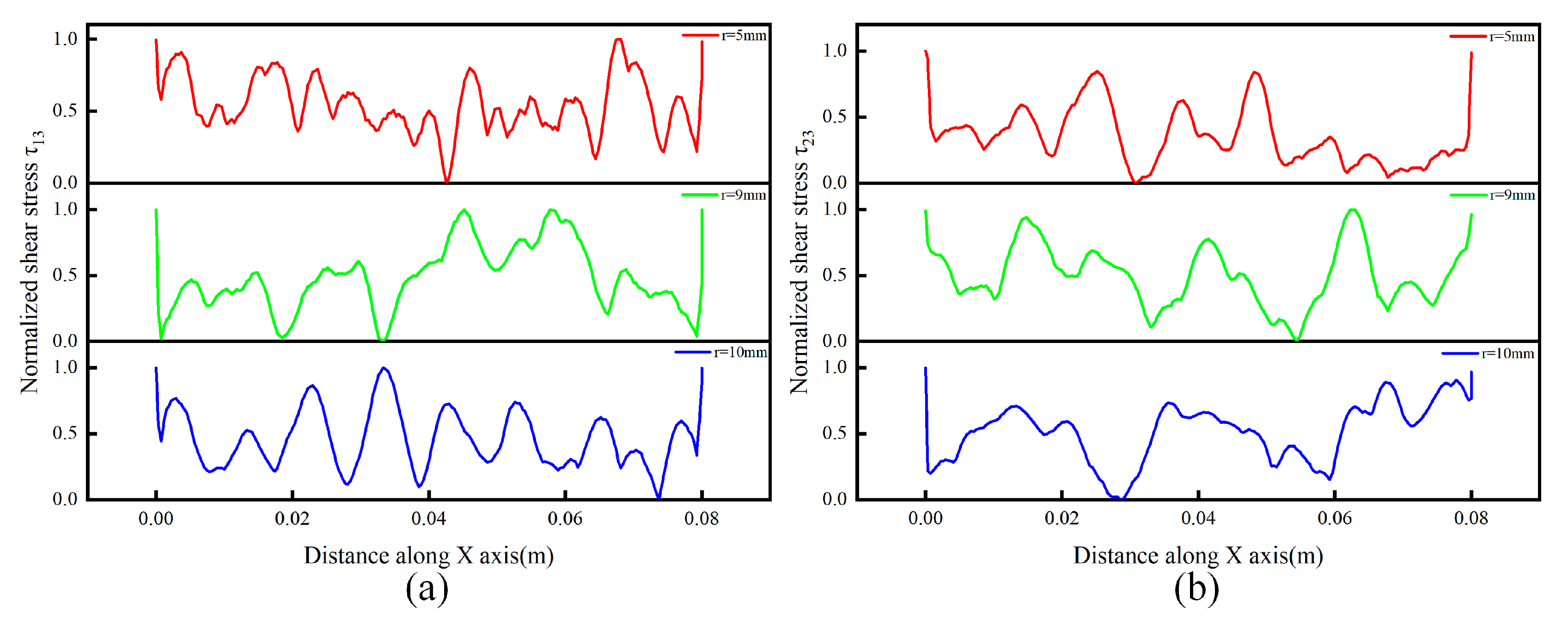
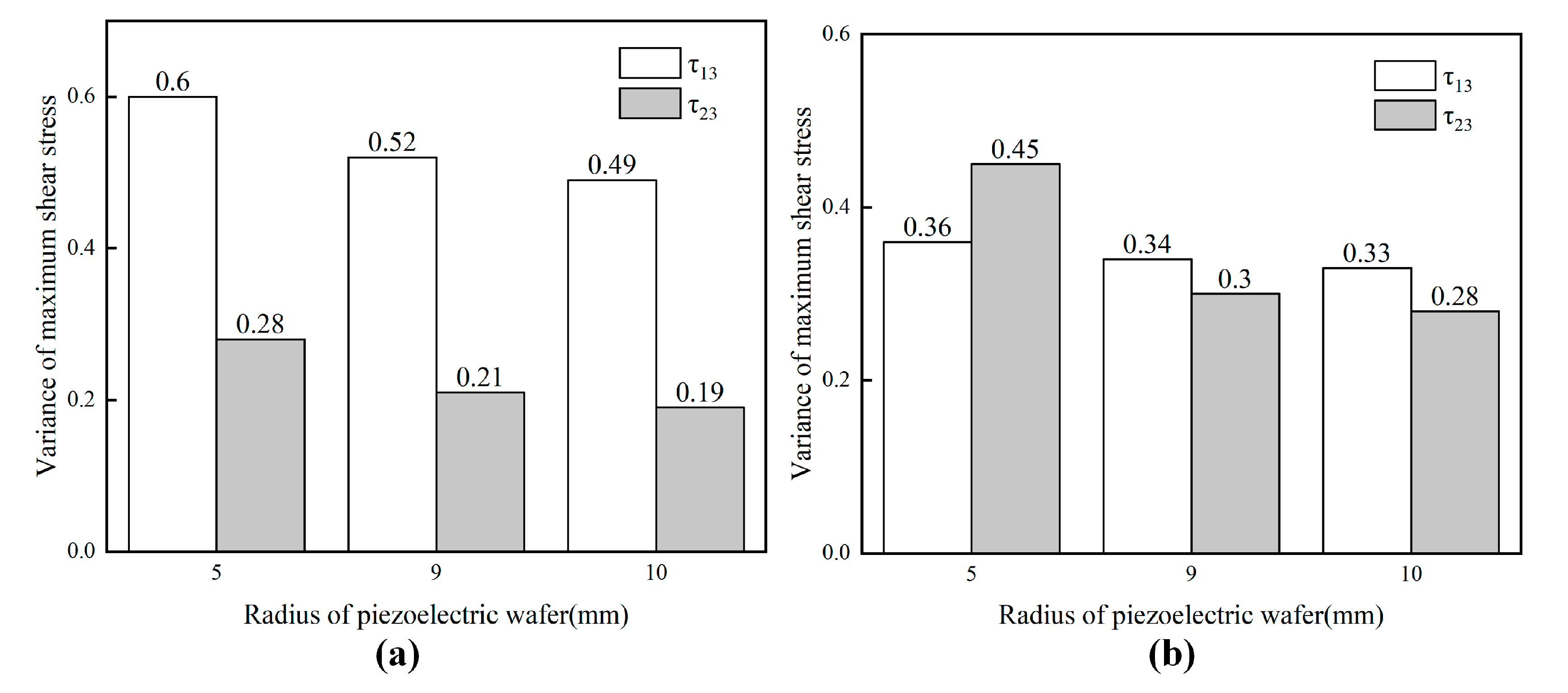
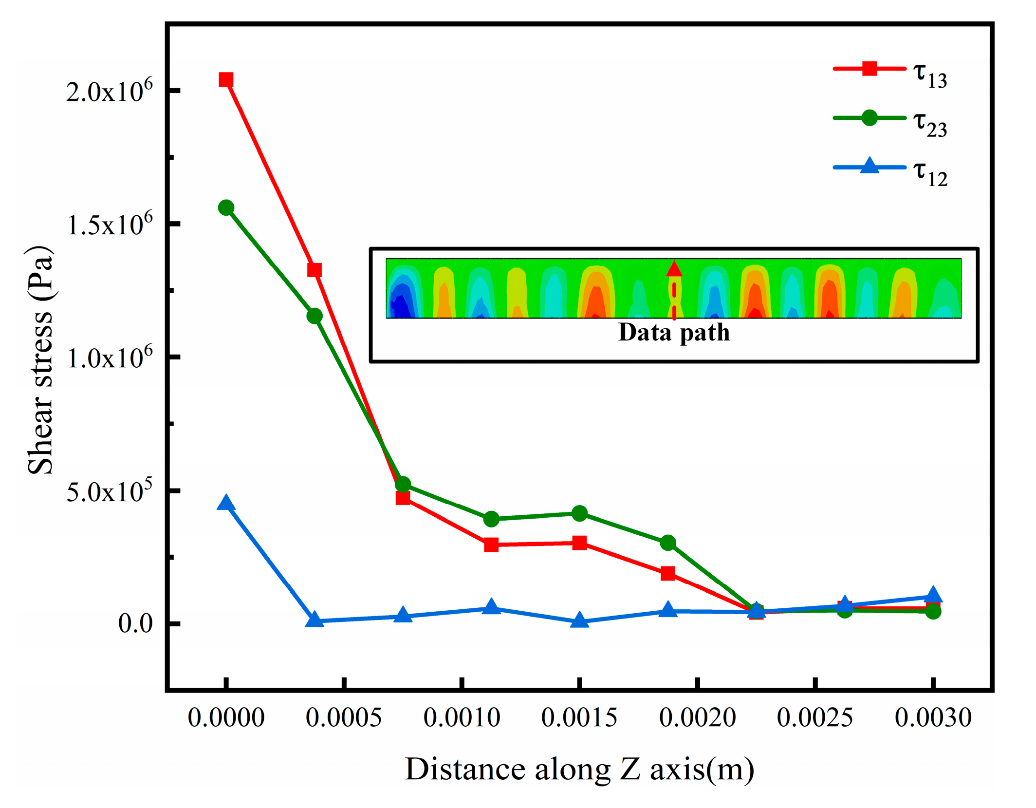
4.2. Stress Distribution and Deicing Affect Analysis

The following study revolved around configuration 2. Stress distribution of ice layer was mainly investigated in this section. The ice/substrate interface shear stress nephogram at XZ plane and YZ plane at frequency 213 kHz were studied. In order to show these results more intuitively, 13 paths at the interface of the ice layer including left and right boundaries were established along the long side of the ice layer, which were parallel to the Y axis. Similarly, 22 paths at the interface of the ice layer including two boundaries were established along the short side of ice layer, which were parallel to the X axis. Based on these, the variations of shear stress with paths can be obtained. Then, the shear stress amplitude of 13 paths parallel to the Y axis and 22 paths parallel to the X axis were averaged separately. Average the shear stress amplitude of 13 paths parallel to the Y axis, the average shear stress τ₁₃ and τ₂₃ vary along the Y axis can be calculated. Similarly, the results of average shear stress amplitude vary along the X axis can also be estimated. The results are shown in Figure 11.

From the simulation results of Figure 11a,b, the conclusion can be drawn that the average shear stress τ₁₃ and τ₂₃ amplitudes are symmetric about the neutral axis. Combining these two figures results with shear stress nephogram, it can be found that τ₁₃ is symmetric about the neutral axis, while τ₂₃ is antisymmetric about the neutral axis. From the results of Figure 11, it can be seen that the average shear stresses are higher at edges and corners of the ice layer which means ice debonding starts from the edges and corners of the ice layer. Meanwhile, the shear stress distributions of deicing efficiency top three, configuration 2 (r = 5 mm), configuration 6 (r = 9 mm), and configuration 7 (r = 10 mm) were compared. In order to find the principle of stress distributions of these three configurations, the shear stress τ₁₃ and τ₂₃ were normalized. The results are shown in Figure 12 and Figure 13.

Figure 12 and Figure 13 reveal the relationship between shear stress distribution and deicing efficiency. The normalized shear stress distribution can reflect the stress gradient from edges to the center of the ice layer. In order to describe this type of stress gradient, a coefficient by referring to the definition of variance was defined. The coefficient named variance of maximum shear stress (VMSS) represents the degree of dispersion between shear stress at the edges and middle of the ice layer. For the average shear stress at the edges of the ice layer at maximum, the average shear stress at the edges would be equal to one after normalization. Thus, this coefficient can be described as Formula (13):

$$\mathrm{VMSS}=\frac{1}{N}{\displaystyle \sum _{i=1}^N({\tau }_i}-{\tau }_{max}{)}^2=\frac{1}{N}{\displaystyle \sum _{i=1}^N({\tau }_i}-1{)}^2,$$

(13)

where N, τ_i represent the number of node and shear stress for each node, respectively, τ_max means shears stress at edges, which equals to one after normalization. The larger the value of VMSS, the larger the degree of dispersion. That presents the shear stresses at the edges of the ice layer reach the deicing stress threshold, the shear stresses at the rest of the part of the ice layer are still relatively small. It means shear stresses are more concentrated on the edges, which is more efficiency and power saving. The results for these three configurations are shown in Figure 14.

In Figure 14, coefficient VMSS shows a downward trend from configuration 2 (r = 5 mm), configuration 6 (r = 9 mm) to configuration 7 (r = 10 mm). This conclusion is consistent with the results of coefficient DEF, which proves the correctness of DEF from another perspective. In addition, 15 paths along the thickness direction of the ice layer were established to analyze the shear stress distribution along the Z axis direction. The results are shown in Figure 15.

The result of Figure 15 shows that amplitude of shear stress τ₁₃ and τ₂₃ decrease from interface to free surface while shear stress τ₁₂ exists along the entire thickness direction of ice layer, which is corresponding with theory and analysis.

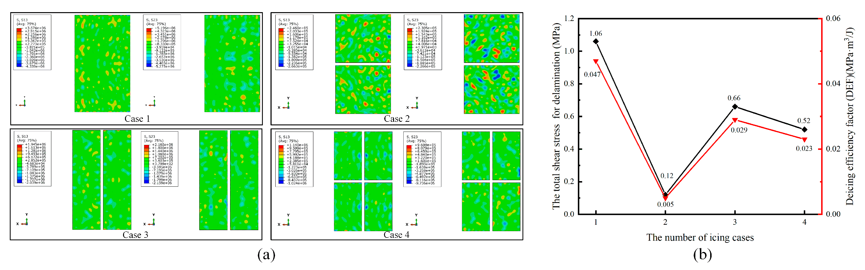
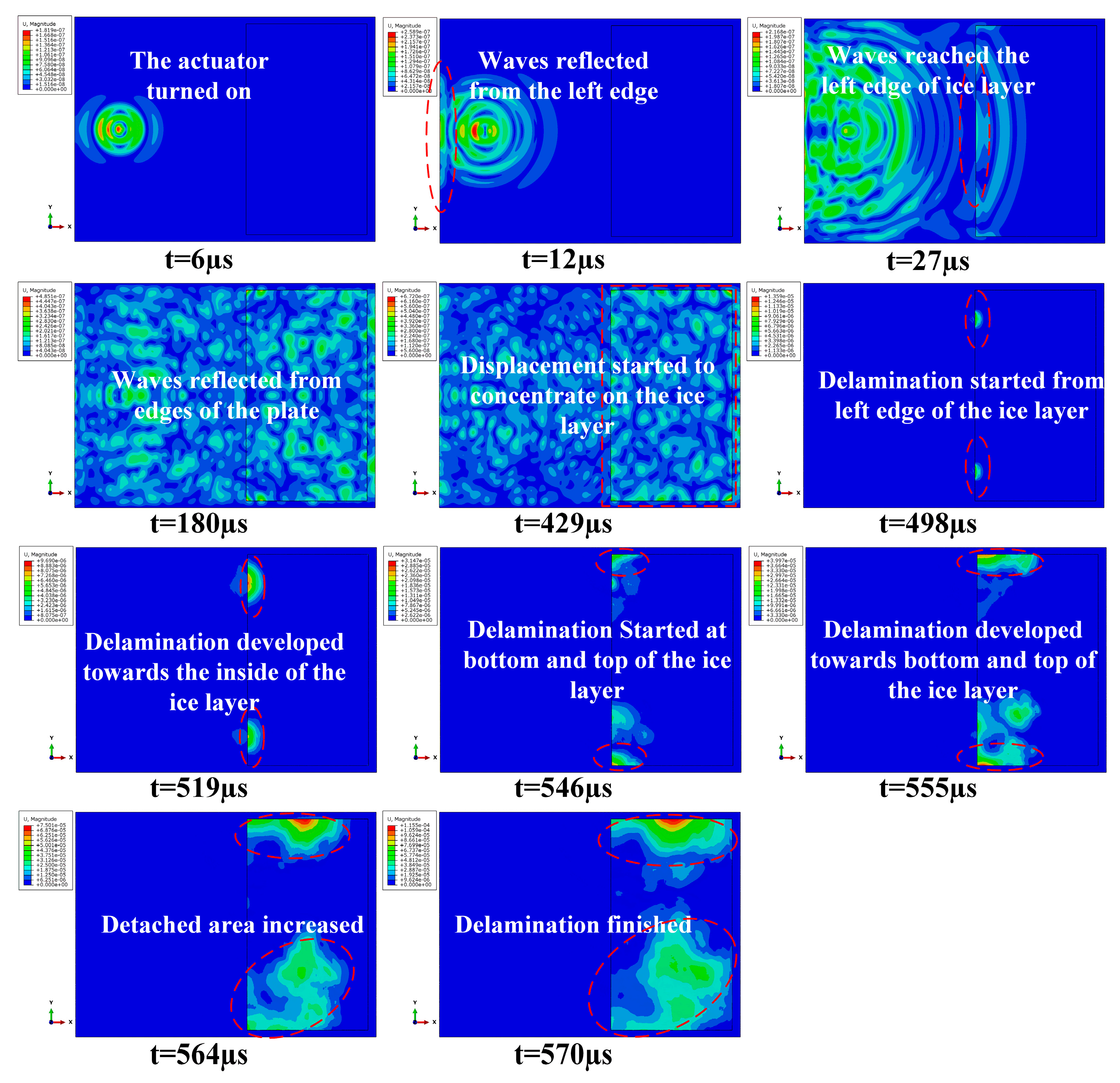
4.3. Standard-Explicit Co-Simulation Analysis

With the help of transient dynamic analysis by using standard-explicit co-simulation, the whole process of wave propagation and deicing can be revealed more clearly. Similarly, configuration 2 was studied in the process. The distribution of displacement for the aluminum plate and ice layer at different times was calculated and shown in Figure 16. After the PZT actuator was turned on 6 μs, waves were generated and started to spread around the actuator. After 12 μs, waves reached and reflected from the left edge of the aluminum plate. Then, the reflected waves were superimposed with waves generated by the actuator and propagated toward the ice layer. Around 27 μs later, waves reached the left edge of the ice layer. In the process, the waves continued spreading to the right edge of the aluminum plate and reflected from the edges around 180 μs. Gradually, displacement started to concentrate on the ice layer after 429 μs. Then, 498 μs later, the left edge of ice layer started to peel off symmetrically along the neutral axis of the aluminum plate. Delamination developed towards the inside of the ice layer within 519 μs. After that, delamination started at the bottom and top of the ice layer about 546 μs. Then, detachment developed towards the bottom and top of the ice layer after 555 μs. After 564 μs, detachment developed to the center and right edge of the ice layer. Finally, delamination finished at 570 μs.

To reveal the deicing process more clearly, an index for damage degree (SDEG) was utilized to elaborate the interface damage evolution process. Figure 17 shows the evolution process of SDEG for the cohesive layer. When SDEG was equal to 1, the area was detached and deleted. After the actuator was turned on 450 μs, damage initiation occurred at the left, bottom, and top edge of the cohesive layer. After 498 μs, the left edge of the cohesive layer started to damage and deleted. The ice layer stared to detach from the aluminum plate. Then, damage developed along the wave propagation direction after 531 μs. With the evolution of damage, the bottom and top of the ice layer was peeled off at 549 μs. Then, the detached area continued to increase. The detachment developed to the center and right edge of the ice layer around 564 μs. Finally, the delamination finished within 570 μs. The detachment area was around 88.2% of the icing area. Although the ice layer was not totally detached, the remaining area of the cohesive layer also showed varying degrees of damage, which meant that the ice layer was likely to be removed completely under a small external load.

Based on results of dynamic analysis, the processes of wave propagation, reflection, and superposition can be better observed and understood. Besides, the entire peeling process of the ice layer can be studied and presented. From the results of the above simulation, it can be found that the detachment started at the edge of the ice layer, which coincided with the stress distribution analysis in Section 4.2. In the harmonic analysis for configuration 2, the detached area was 83.3%. In the above dynamic analysis, the detached area was 88.2%. It showed that good agreements between these two analyses were obtained.

4.4. Experimental Verification

The deicing results for configuration 2 are shown in Figure 18. Three deicing experiments under different frequencies were compared. When frequency was 190 kHz, there was no visible change observed. When frequency was 236 kHz, only some cracks but without any delamination were observed. When frequency was 213 kHz, the ice layer was cracked and partially detached from the aluminum plate. After the actuator was turned on 24 s, delamination started from the edge of the ice layer. The delamination area increased along the wave propagation direction with some cracks after 47 s. Then, the detached area continued to increase with more cracks generated. Finally, delamination finished within 71 s. The detached area could be estimated from the nephogram in an open source image processing software named ImageJ [35]. Firstly, the experimental results image was converted into grayscale images. The detached area can be identified by comparing the images before and after the experiment. Then, the color threshold was set according to the color of the detached area. Based on these, the detached area was calculated. In the ice layer nephogram, the detached area was in white. The percent of shear stress exceeded the adhesion stress at 83.3% and 88.2% in harmonic analysis and dynamic analysis while it was 76.4% in the experiment. The main error came from the difference in ice properties between the simulation and experiment.

Simultaneously, the different performances at frequency 190 and 236 kHz were also corresponding with simulation results. The final results are shown in

Table 4. Comparison of experimental and simulation results for three different frequencies.

Frequency (kHz)	Experimental Results	Simulation Results
190	Without visible change	Maximum τtotal = 0.23 MPa; Maximum τ12 = 0.11 MPa
213	Ice delamination and cracking	Maximum τ13 = 4.3 MP; Detached area is 83.3%; Maximum τ12 = 3.0 MPa
236	Cracks only	Maximum τtotal = 0.16 MPa; Maximum τ12 = 0.28 MPa

. Neither frequency, 190 nor frequency 236 kHz could detach the ice layer, since both shear stresses of them were smaller than the adhesion strength of the ice. The crack existed at frequency 236 kHz rather frequency 190 kHz due to shear stress τ₁₂ which contributed to ice cracking. Shear stress τ₁₂ was higher at frequency 236 than 190 kHz. Thus, the crack could observe at frequency 236 kHz rather than 190 kHz.

Meanwhile, deicing experiments were also performed for the remaining six groups at their optimal frequency, respectively. The trend of detached areas after deicing experiments and total shear stress τ_total for delamination from FE simulation results were compared. The trend of total shear stress τ_total and the detached area are shown in Figure 19.

The result of Figure 19 can prove the optimal frequency for configuration 2 was 213 kHz. From the results of Figure 19, it can be found that the trend of detached areas in experiments is consistent with total shear stress in FE simulations, which can verify the correctness of FE simulation results and feasible of the deicing method. Finally, deicing experiments for four different icing cases mentioned before were conducted. The deicing results for these four cases are shown in Figure 20. The trend of the detached area for these four cases is consistent with the trend of DEF predicted in the FE simulation.

5. Conclusions

In this paper, a flat deicing system using ultrasonic waves to detach the ice layer from the host structure was studied. The feasibility of the deicing system was validated in both FE simulations and experiments. In FE simulations, both harmonic analysis and dynamic analysis were conducted. In the harmonic analysis, deicing parameters and deicing frequencies were given. For different configuration, a factor (DEF) was proposed to estimate and predict deicing efficiency. Based on optimal configuration, four icing cases were discussed for further validation of DEF. Simultaneously, the relationship between shear stress distributions and deicing was explored. In dynamic analysis, wave propagation and the deicing process were investigated. Finally, deicing experiments were performed to verify the feasibility of the deicing system and the reasonableness of predicted results in FE simulations.

Based on the results above, the following conclusions were drawn:

• A parameter design method was proposed according to simulation results on the supercomputer. The optimal configuration (the radius and the thickness of the PZT actuator) and deicing frequency were also given.
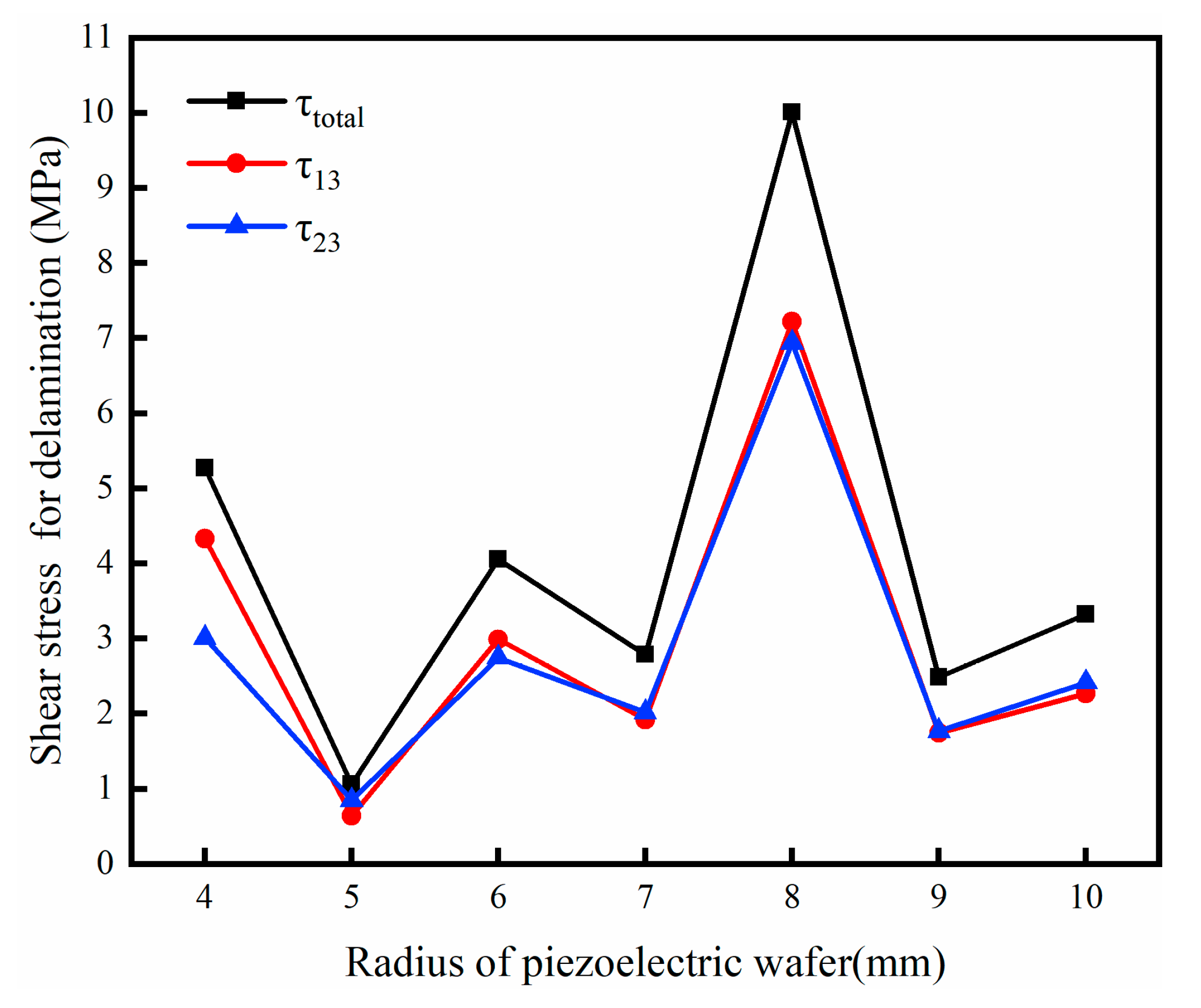
• The coefficient deicing efficiency factor (DEF) was proposed based on FE simulation, which can estimate and predict the deicing efficiency. With the help of this factor, the effect of the different model and deicing parameters on deicing efficiency can be calculated and compared. For shear stresses distributions, the more concentrated the shear stresses are on the edges of ice/substrate interface, the better for deicing. This can be one of the potential ways to achieve deicing more effectively.
• The calculation results of harmonic analysis and dynamic analysis are consistent. Harmonic analysis can obtain deicing stress and deicing results more concise and clearer. Wave propagation, reflection, superposition, and other processes are better displayed in dynamic analysis, which can help to understand the deicing process and provide guidance for further optimization. For different models and problems, these two analyses should be used rationally to achieve the purpose of obtaining the expected results with lower calculation costs.

References

1. Cao, Y.; Tan, W.; Wu, Z. Aircraft icing: An ongoing threat to aviation safety. Aerosp. Sci. Technol. 2018, 75, 353–385. [Google Scholar] [CrossRef]
2. Nadeau, S.; Morency, F. De-icing of aircraft: Incorporating business risks and occupational health and safety. Int. J. Saf. Secur. Eng. 2017, 7, 247–266. [Google Scholar] [CrossRef] [Green Version]
3. Yirtici, O.; Ozgen, S.; Tuncer, I.H. Predictions of ice formations on wind turbine blades and power production losses due to icing. Wind Energy 2019, 22, 945–958. [Google Scholar] [CrossRef]
4. Jin, J.Y.; Virk, M.S. Study of ice accretion and icing effects on aerodynamic characteristics of DU96 wind turbine blade profile. Cold Reg. Sci. Technol. 2019, 160, 119–127. [Google Scholar] [CrossRef]
5. Samuelsen, E.M. Ship-icing prediction methods applied in operational weather forecasting. Q. J. R. Meteorol. Soc. 2018, 144, 13–33. [Google Scholar] [CrossRef]
6. Dehghani-Sanij, A.; Dehghani, S.; Naterer, G.; Muzychka, Y. Marine icing phenomena on vessels and offshore structures: Prediction and analysis. Ocean Eng. 2017, 143, 1–23. [Google Scholar] [CrossRef]
7. Wei, K.; Yang, Y.; Zuo, H.; Zhong, D. A review on ice detection technology and ice elimination technology for wind turbine. Wind Energy 2020, 23, 433–457. [Google Scholar] [CrossRef]
8. Fakorede, O.; Feger, Z.; Ibrahim, H.; Ilinca, A.; Perron, J.; Masson, C. Ice protection systems for wind turbines in cold climate: Characteristics, comparisons and analysis. Renew. Sustain. Energy Rev. 2016, 65, 662–675. [Google Scholar] [CrossRef]
9. Goraj, Z. An overview of the deicing and anti-icing technologies with prospects for the future. In Proceedings of the 24th International Congress of the Aeronautical Sciences, Yokohama, Japan, 29 August–3 September 2004. [Google Scholar]
10. Ramanathan, S. An Investigation on the Deicing of Helicopter Blades Using Shear Horizontal Guided Waves. Ph.D. Thesis, The Pennsylvania State University, University Park, PA, USA, 2004. [Google Scholar]
11. Palacios, J.; Smith, E.; Rose, J.; Royer, R. Instantaneous de-icing of freezer ice via ultrasonic actuation. AIAA J. 2011, 49, 1158–1167. [Google Scholar] [CrossRef] [Green Version]
12. Seppings, R.A. Investigation of Ice Removal from Cooled Metal Surfaces. Ph.D. Thesis, Imperial College London (University of London), London, UK, 2006. [Google Scholar]
13. Yin, C.; Zhang, Z.; Wang, Z.; Guo, H. Numerical simulation and experimental validation of ultrasonic de-icing system for wind turbine blade. Appl. Acoust. 2016, 114, 19–26. [Google Scholar] [CrossRef]
14. Budinger, M.; Pommier-Budinger, V.; Napias, G.; Costa da Silva, A. Ultrasonic Ice Protection Systems: Analytical and Numerical Models for Architecture Tradeoff. J. Aircr. 2016, 53, 680–690. [Google Scholar] [CrossRef] [Green Version]
15. Kalkowski, M.K.; Waters, T.P.; Rustighi, E. Delamination of surface accretions with structural waves: Piezo-actuation and power requirements. J. Intell. Mater. Syst. Struct. 2017, 28, 1454–1471. [Google Scholar] [CrossRef]
16. Shi, Z.; Zhao, Y.; Ma, C.; Zhang, J. Parametric Study of Ultrasonic De-Icing Method on a Plate with Coating. Coatings 2020, 10, 631. [Google Scholar] [CrossRef]
17. Zhu, Y. Structural Tailoring and Actuation Studies for Low Power Ultrasonic De-Icing of Aluminum and Composite Plates. Ph.D. Thesis, The Pennsylvania State University, University Park, PA, USA, 2010. [Google Scholar]
18. DiPlacido, N.; Soltis, J.; Palacios, J. Enhancement of ultrasonic de-icing via tone burst excitation. J. Aircr. 2016, 53, 1821–1829. [Google Scholar] [CrossRef]
19. Wang, Z.; Xu, Y.; Gu, Y. A light lithium niobate transducer design and ultrasonic de-icing research for aircraft wing. Energy 2015, 87, 173–181. [Google Scholar] [CrossRef]
20. Gao, H.; Rose, J.L. Ice detection and classification on an aircraft wing with ultrasonic shear horizontal guided waves. IEEE Trans. Ultrason. Ferroelectr. Freq. Control. 2009, 56, 334–344. [Google Scholar]
21. Palacios, J.; Zhu, Y.; Smith, E.; Rose, J. Ultrasonic shear and lamb wave interface stress for helicopter rotor de-icing purposes. In Proceedings of the 47th AIAA/ASME/ASCE/AHS/ASC Structures, Structural Dynamics, and Materials Conference, Newport, RI, USA, 1–4 May 2006; p. 2282. [Google Scholar]
22. Daniliuk, V.; Xu, Y.; Liu, R.; He, T.; Wang, X. Ultrasonic de-icing of wind turbine blades: Performance comparison of perspective transducers. Renew. Energy 2020, 145, 2005–2018. [Google Scholar] [CrossRef]
23. Elices, M.; Guinea, G.; Gomez, J.; Planas, J. The cohesive zone model: Advantages, limitations and challenges. Eng. Fract. Mech. 2002, 69, 137–163. [Google Scholar] [CrossRef]
24. Alfano, G.; Sacco, E. Combining interface damage and friction in a cohesive-zone model. Int. J. Numer. Methods Eng. 2006, 68, 542–582. [Google Scholar] [CrossRef]
25. Li, S. Piezoelectric Fiber Composite Strip Health Monitoring Systems Based on Ultrasonic Guided Waves. Master’s Thesis, The Pennsylvania State University, University Park, PA, USA, 2011. [Google Scholar]
26. Wang, T. Finite Element Modelling and Simulation of Guided Wave Propagation in Steel Structural Members. Ph.D. Thesis, University of Western Sydney, Sydney, Australia, 2014. [Google Scholar]
27. Rose, J.L. Ultrasonic Guided Waves in Solid Media; Cambridge University Press: Cambridge, UK, 2014. [Google Scholar]
28. Centolanza, L.R.; Smith, E.C.; Munsky, B. Induced-shear piezoelectric actuators for rotor blade trailing edge flaps. Smart Mater. Struct. 2002, 11, 24. [Google Scholar] [CrossRef]
29. Kandagal, S.; Venkatraman, K. Piezo-actuated vibratory deicing of a flat plate. In Proceedings of the 46th AIAA/ASME/ASCE/AHS/ASC Structures, Structural Dynamics and Materials Conference, Austin, TX, USA, 18–21 April 2005; p. 2115. [Google Scholar]
30. Systèmes, D. Abaqus analysis user’s guide. Solid (Contin.) Elem. 2014, 6, 2019. [Google Scholar]
31. Riahi, M.M.; Marceau, D.; Laforte, C.; Perron, J. The experimental/numerical study to predict mechanical behaviour at the ice/aluminium interface. Cold Reg. Sci. Technol. 2011, 65, 191–202. [Google Scholar] [CrossRef]
32. Mlyniec, A.; Ambrozinski, L.; Packo, P.; Bednarz, J.; Staszewski, W.J.; Uhl, T. Adaptive de-icing system–numerical simulations and laboratory experimental validation. Int. J. Appl. Electromagn. Mech. 2014, 46, 997–1008. [Google Scholar] [CrossRef]
33. Wei, Y.; Adamson, R.; Dempsey, J. Ice/metal interfaces: Fracture energy and fractography. J. Mater. Sci. 1996, 31, 943–947. [Google Scholar] [CrossRef]
34. Guerin, F.; Laforte, C.; Farinas, M.-I.; Perron, J. Analytical model based on experimental data of centrifuge ice adhesion tests with different substrates. Cold Reg. Sci. Technol. 2016, 121, 93–99. [Google Scholar] [CrossRef]
35. Schneider, C.A.; Rasband, W.S.; Eliceiri, K.W. NIH Image to ImageJ: 25 years of image analysis. Nat. Methods 2012, 9, 671–675. [Google Scholar] [CrossRef]
Figure 1. The coordinate system and ultrasonic waves propagating in the ice-plate layered structure.
Applsci 10 06640 g001
Figure 2. The 3D model of finite element simulation.
Applsci 10 06640 g002
Figure 3. Phase velocity of the aluminum plate and ice-plate layered structure: (a) 2 mm aluminum plate, (b) 2 mm aluminum plate with 3 mm ice.
Applsci 10 06640 g003
Figure 4. FE mesh and reference points (A and B) of the deicing system for the FE parametric study.
Applsci 10 06640 g004
Figure 5. Different icing cases for configuration 2: (a) One ice block; (b) Two ice blocks separated along X axis; (c) Two ice blocks separated along Y axis; (d) Four ice blocks.
Applsci 10 06640 g005
Figure 6. Experimental setup for deicing experiments.
Applsci 10 06640 g006
Figure 7. Shear stress amplitude-frequency curves of node: (a) node A (edge point); (b) node B (middle point).
Applsci 10 06640 g007
Figure 8. Shear stress for delamination of seven different configuration.
Applsci 10 06640 g008
Figure 9. Energy density needed for deicing and deicing efficiency factor (DEF) of seven different configurations.
Applsci 10 06640 g009
Figure 10. (a) Ice/substrate interface shear stress nephogram for four different icing cases; (b) The total shear stress for delamination and deicing efficiency factor for the four icing cases.
Applsci 10 06640 g010
Figure 11. Average shear stress amplitude varies along the axis direction: (a) τ13 amplitude varies along the Y axis; (b) τ23 amplitude varies along the Y axis; (c) τ13 amplitude varies along the X axis; (d) τ23 amplitude varies along the X axis.
Applsci 10 06640 g011
Figure 12. Normalized shear stress amplitude varies along the Y axis: (a) shear stress τ13; (b) shear stress τ23.
Applsci 10 06640 g012
Figure 13. Normalized shear stress amplitude varies along the X axis: (a) shear stress τ13; (b) shear stress τ23.
Applsci 10 06640 g013
Figure 14. Variance of maximum shear stress along Y axis (a) and X axis (b).
Applsci 10 06640 g014
Figure 15. Average shear stress amplitude varies along the Z axis.
Applsci 10 06640 g015
Figure 16. Displacement distribution for the aluminum plate and ice layer over time.
Applsci 10 06640 g016
Figure 17. Cohesive layer damage evolution process.
Applsci 10 06640 g017
Figure 18. Deicing effects for different frequencies.
Applsci 10 06640 g018
Figure 19. The trend of total shear stress τtotal and detached area.
Applsci 10 06640 g019
Figure 20. The trend of detached area and deicing efficiency factor (DEF) for four different icing cases.
Applsci 10 06640 g020