Mooring-Failure Monitoring of Submerged Floating Tunnel Using Deep Neural Network

Abstract

This paper presents a machine learning method for detecting the mooring failures of SFT (submerged floating tunnel) based on DNN (deep neural network). The floater-mooring-coupled hydro-elastic time-domain numerical simulations are conducted under various random wave excitations and failure/intact scenarios. Then, the big-data is collected at various locations of numerical motion sensors along the SFT to be used for the present DNN algorithm. In the input layer, tunnel motion-sensor signals and wave conditions are inputted while the output layer provides the probabilities of 21 failure scenarios. In the optimization stage, the numbers of hidden layers, neurons of each layer, and epochs for reliable performance are selected. Several activation functions and optimizers are also tested for the present DNN model, and Sigmoid function and Adamax are respectively adopted to enhance the classification accuracy. Moreover, a systematic sensitivity test with respect to the numbers and arrangements of sensors is performed to find the appropriate sensor combination to achieve target prediction accuracy. The technique of confusion matrix is used to represent the accuracy of the DNN algorithms for various cases, and the classification accuracy as high as 98.1% is obtained with seven sensors. The results of this study demonstrate that the DNN model can effectively monitor the mooring failures of SFTs utilizing real-time sensor signals.

1. Introduction

SFT (Submerged floating tunnel) is an alternative infrastructure to conventional/floating bridges and immersed tunnels for deep-sea crossing. It is balanced underwater by its buoyancy, weight, and constraint forces by means of mooring systems [1]. Feasibility studies of SFT have been performed by many researchers worldwide based on its potential advantages such that SFT can be safe in both waves and earthquakes since wave loads exponentially decay with submergence depth and seismic excitations are indirectly transmitted through flexible moorings [2]. However, the real SFT construction is not realized since its safety and feasibility are not fully guaranteed yet. Since the structure is deeply submerged, its structural health monitoring is another big challenging area. In this regard, the present paper focuses on smart structural health monitoring to design safer and more reliable SFTs in the future.

Two major investigations are essential in the design and operation of SFT for its safety and reliability. First, in the design stage, dynamic and structural analyses are needed under various environmental conditions and scenarios. Environmental loads include waves, earthquakes, currents, and tsunamis. Among them, waves tend to be the most important environmental loading if the submergence depth is not sufficiently large [3,4,5,6,7]. For SFT with a large diameter, it was found through hydro-elastic analysis that large static and dynamic mooring tensions were critical issues [7]. To solve this, various design concepts were suggested, e.g., variable-span mooring design [7] and suspension-cable type [8]. However, despite the effort to reduce mooring tension, there still exist several uncertainties, such as nonlinear SFT behaviors and related snap loading that can lead to unexpectedly large tension. In such a case, unexpected mooring failure can potentially happen. Similarly, collisions and underwater explosions can break mooring lines. Second, when any mooring failure happens, it has to be rapidly detected to avoid further problems. Since SFTs are not visible, the detection is not that simple. Diverse monitoring systems have been suggested for underwater flexible systems. The most direct method is to use ROVs (remotely operated vehicles); however, they are expensive and continuous real-time monitoring is not possible. The beam-theory-and-sensor-based monitoring systems with accelerometers/strain gauges [9] and inclinometers/GPS were developed [10]. These methods need mode shapes or structural parameters in advance. Other researchers also used analytical, transfer-function, and mode-matching methods for riser monitoring [11]. However, the above methods still require many sensors to predict global behaviors and local failures.

Recently, ML (machine learning) has newly been employed for the smart monitoring of marine structures. While the above conventional methods require a lot of sensors to monitor potential failures, machine-learning-based algorithms can accurately detect problems with the fewer number of sensors. For example, Chung et al. [12] performed analyses to detect the damage of TLP (tension leg platform) mooring by using DNN (deep neural networks). Jaiswal and Ruskin [13] presented the development of a machine learning algorithm for mooring-failure detection using measured vessel positions and 6-DOF acceleration data. Sidarta et al. [14] developed an ANN (artificial neural network) algorithm for detecting broken mooring lines for FPSO (floating production storage and offloading). Sidarta et al. [15] also developed a machine-learning-based algorithm for detecting mooring-line failures of a semi-submersible. The above examples utilized floaters’ motions to detect mooring-line failures so that much fewer sensors can be used compared to the conventional deterministic methods. They [12,13,14,15] also assumed that floating structures are rigid to simplify the analyses of motion-sensor signals.

In this study, we developed a ML-based mooring-failure-monitoring system for a long and highly flexible SFT with DNN algorithms to detect mooring-line failures in real time without employing human effort or any devices. The effects of variable number of sensors (accelerometers) and their locations were analyzed. The training data for the developed ML algorithm was produced by running the author-developed time-domain SFT simulation program [7] using the commercial software, OrcaFlex [16]. The simulations of SFT’s wave-induced motions and mooring tensions were partly validated through comparisons with an independent SFT hydro-elastic simulation program [7,17] and a series of experimental results with small SFT sections [18]. To validate the developed smart monitoring system, various intact/failure scenarios and wave conditions were considered for training and testing of the algorithm. In the algorithm optimization stage, not only the numbers of the hidden layers, neurons, and epochs but also the activation function and optimizer were properly utilized to enhance the detection accuracy. Contrary to previous researches [12,13,14,15], in the case of highly elastic SFT, a single sensor cannot cover the entire motion, so several sensors are required, as presented in [19]. In this regard, in the testing stage, we checked the detection accuracy of the developed algorithm with different numbers and arrangements of sensors. Machine learning algorithms for the failure detection of submerged deformable structures like SFT have rarely been investigated in the open literature. In this regard, this study using DNN will help other researchers to investigate similar problems in the future.

2. Numerical Model

2.1. Submerged Floating Tunnel

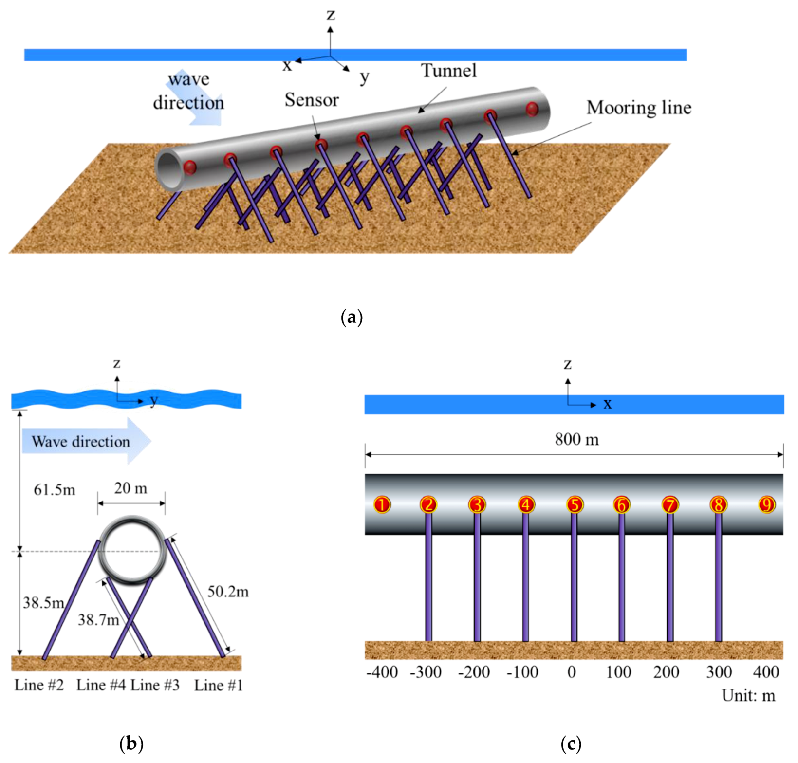
We considered SFT with 28 mooring lines as an example, as shown in Figure 1. Material properties and design parameters are presented in Table 1. The tunnel, 20 m in diameter and 800 m in length, is made of high-density concrete. BWR (buoyancy weight ratio) is set as 1.3. We assume that the tunnel has fixed stations at both ends and water depth is constant at 100 m. The submergence depth, which is a vertical distance between the MWL (mean water level) and the tunnel centerline, is set at 61.5 m. As can be seen in Figure 1, four 60-degree inclined mooring lines made of studless chains are installed with 100-m interval along the longitudinal length. The lengths of the mooring lines are 50.2 m for lines #1 and #2 and 38.7 m for lines #3 and #4. In addition, accelerometers are located along the tunnel’s centerline, as shown in Figure 1c. We conduct a systematic sensitivity test with respect to the numbers and arrangements of accelerometers, as discussed in Section 4.3.

Figure 1. 2D and 3D schematic drawings (accelerometers are marked with red dots in (a); mooring line numbers are given in (b); sensor numbers (1–9) are given in (c)).

Table 1. Design parameter of the SFT (E is Young’s modulus, I is area moment of inertia, A is cross-sectional area).

Parameter	Value	Unit
Tunnel length	800	m
Tunnel diameter	20	m
Interval of mooring lines	100	m
End boundary condition	Fixed-fixed	-
Material of tunnel	High-density concrete	-
Length of mooring lines	50.2 (line #1,2), 38.7 (line #3,4)	m
Added mass coefficient	1.0	-
Nominal diameter of mooring lines	0.18	m
Drag coefficient	0.55 (tunnel), 2.4 (mooring lines)	-
Bending stiffness (EI)	1.34 × 1011 (tunnel), 0 (mooring lines)	kN·m2
Axial stiffness (EA)	3.23 × 109 (tunnel), 2.77 × 106 (mooring lines)	kN

2.2. Time-Domain Numerical Simulation

Authors developed a numerical model [7] that can perform tunnel-mooring-coupled time-domain simulations using OrcaFlex [16] to produce data-sets for machine learning. The SFT was modeled by the long-beam model, which consists of nodes (lumped masses) and segments (massless linear and rotational springs). The mass, drag, and other important properties are all lumped at the nodes, and stiffness properties are modeled in the segments. The time-domain equation of motion for SFT can be expressed as:

$$M\ddot{x}+Kx=F_M+w+F_C\delta \left(x_i-\xi \right)$$

(1)

where M and K are system’s mass and structural stiffness matrices, respectively, x is the displacement vector, x_i is the longitudinal position vector of tunnel nodes, ξ is the vector representing longitudinal locations of mooring lines, F_M is the hydrodynamic force vector, w is the wet-weight vector (i.e., net sum of weight and buoyancy), F_C is the constraint force vector at the tunnel-mooring connection locations (i.e., coupling force induced by mooring lines on the tunnel and vice versa), and δ is the Dirac delta function. Upper dot in the equations means time derivative of a variable.

The line’s elastic behaviors are considered by the Kx term with axial, bending, and torsional springs. The axial and torsional springs located at the center of two neighboring nodes evaluate the tension force and torsional moment while the rotational springs located at either side of the node estimate the shear force and bending moment.

The hydrodynamic force at nodes’ instantaneous locations was evaluated by the Morison equation for a moving body, which can be written for a cylindrical object as:

$$F_M=-C_A\rho V_{}{\ddot{x}}^n+C_M\rho V_{}{\dot{\mathsf{\eta }}}^n+\frac{1}{2}{C}_D\rho A\left|{\mathsf{\eta }}^n-{\dot{x}}^n\right|\left({\mathsf{\eta }}^n-{\dot{x}}^n\right)$$

(2)

where C_A, C_M, and C_D are the added mass, inertia, and drag coefficients, respectively, V and A stand for the displaced volume and projected area, ρ is density of water, η is velocity of a fluid particle, and superscript n means the normal direction. More details of the numerical model can be found in [7]. The developed SFT dynamics simulation program was partly validated through comparisons with a series of experimental results for a small SFT segment with similar mooring set-up [18].

2.3. Big-Data Generation under Various Environmental Conditions and Failure Scenarios

Big data were generated and collected by using the developed time-domain simulation program under various wave conditions and intact/failure scenarios, as summarized in Table 2 and Table 3. As shown in Figure 1c, we considered accelerometers as sensors. However, we collected displacement signals directly assuming that real-time double integration is feasible with an appropriate bandwidth filter. Then, we conducted a systematic sensitivity test with respect to the arrangements of accelerometers to discover effective sensor combinations. Note that sensors #1 and #9 were not used for the analysis due to the fixed-fixed boundary conditions. As presented in Table 2, 21 intact/failure cases were simulated for 1800 sec with a time interval of 0.2 sec at each environmental condition. The failure cases were simulated by disconnecting the target mooring lines. The wave heading is assumed to be normal to the longitudinal direction of SFT. Based on symmetry, failure scenarios on the half domain were considered. For the random wave-elevation generation, a JONSWAP wave spectrum was utilized, and 100 regular-wave components were superposed to generate the random wave signals. Signal repetition in time histories was avoided through the equal energy method in which each regular wave component has equal spectral energy. Ten wave conditions were considered, as shown in Table 3. The enhancement parameter (γ) of the wave spectrum was fixed at 2.14. The total data points and time were, therefore, 210 (21 scenarios times 10 environmental conditions) and 378,000 sec (210 simulations times 1800 s). As given in Table 3, we employed 80% of data collected from eight environmental conditions for training, and thus the total data points for training were 134 while the number of data points for testing was 76. Data from the first eight environmental conditions were utilized for studies of optimization and failure-detection performance with different arrangements of the sensors. Later, we further tested the feasibility of the algorithm by employing data from the last two environmental conditions not used for training.

Table 2. Mooring-failure scenarios (mooring line number is based on the line number in Figure 1b, In = intact case, All = failure of all mooring lines (# 1, 2, 3, and 4) at their tunnel location).

Item	Failure Case
	1	2	3	4	5	6	7	8	9	10	11	12	13	14	15	16	17	18	19	20	In
Tunnel Location (m)	−300				−200				−100				0				−300	−200	−100	0	-
Mooring Line Number	1	2	3	4	1	2	3	4	1	2	3	4	1	2	3	4	All	All	All	All	-

Table 3. Wave conditions (Tr is training, Te is testing, percentage in bracket denotes the percentage of data used for training or testing).

Significant Wave Height (Hs) (m)	Peak Period (Tp) (s)	Data Usage
1	6	Tr (80%), Te (20%)
1	10.5	Tr (80%), Te (20%)
1	13	Tr (80%), Te (20%)
5	6	Tr (80%), Te (20%)
5	10.5	Tr (80%), Te (20%)
5	13	Tr (80%), Te (20%)
11.7	10.5	Tr (80%), Te (20%)
11.7	13	Tr (80%), Te (20%)
3	8	Te (100%)
7	12	Te (100%)

3. Deep Neural Network

3.1. Artificial Neural Network

ANN is a parallel computational model consisting of adaptive processing units that are densely connected to each other [20]. ANN is a biologically inspired computing method based on the neural structures of the brain. Neurons and layers are basic elements to design a neural network structure. To be specific, a layer consists of a certain number of neurons while neurons in a layer are connected with neurons in neighboring layers linearly. There are three types of layers, i.e., input, hidden, and output layers [21]. When there exist multiple hidden layers, it is called DNN.

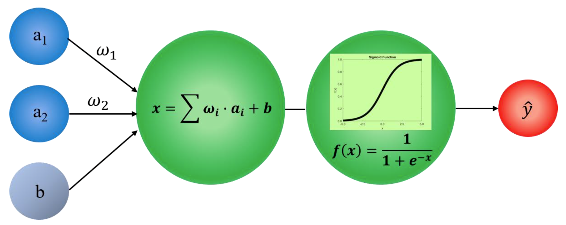
Learning in DNN is a process of determining the weights and biases in each layer so that the error between the final output value and the actual value can be minimized. Figure 2 shows the mechanism of the learning process. This learning procedure is called feedforward because it flows from the input nodes a to the last output $\widehat{y}$ through the intermediate layer where the activation function f(x) exists. The weighted sum of the inputs x is firstly estimated by weights ω, a, and bias b, and activation function decides whether outside connections consider this neuron as activated or not. Finally, the network produces the predicted value $\widehat{y}$ [22]. In this sense, the error of the network is defined as the correct answer y minus the predicted value $\widehat{y}$.

Figure 2. Layout of feedforward algorithm.

Classification learning needs to update the weights based on the error values to enhance accuracy. In this regard, the backpropagation algorithm was adapted. The backpropagation algorithm trains the neural network by backpropagating the error of the output layer to the hidden layers while updating weights and bias. In this study, a delta rule was utilized, which can be expressed as [23,24]:

$${\omega }_{i+1}={\omega }_i+\eta \cdot \delta \cdot a$$

(3)

where η and δ are the learning rate and delta. The learning rate is a parameter of the optimization algorithm that determines the step size at each epoch, moving towards the minimum loss function [24]. Delta is first calculated by multiplying the error value by the derivative of the activation function, and error is then calculated for the next layer as:

$$\delta =f^{\prime }(x)\cdot e$$

(4)

$$e=W^T\delta$$

(5)

where W^T is the transpose of weight matrix {ω₁, ω₂, …, ω_n,}. Delta of the output node is backpropagated to calculate the delta of the hidden nodes while repeating this process of backpropagation to the leftmost hidden layer. The neural network learning of feedforward and backpropagation is repeated until the error converges.

3.2. Neural Network Model Architecture

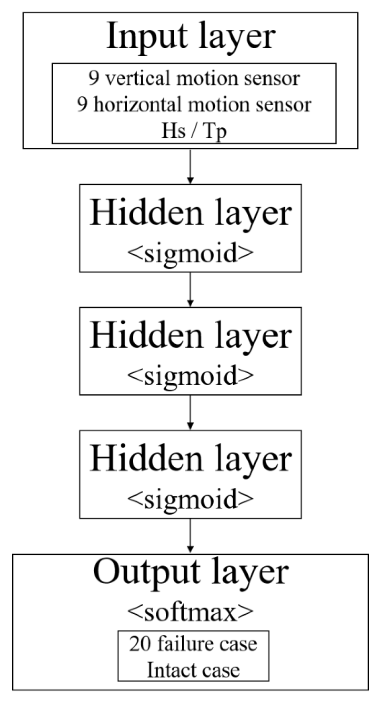
Figure 3 shows the present DNN model for mooring-failure monitoring. In this study, mooring-failure locations are to be predicted by the change of tunnel motion-sensor signals under given wave conditions. In other words, the input layer consists of the tunnel motions from sensors and wave conditions, and the output layer provides the probabilities of 21 failure scenarios. We optimized the number of hidden layers and neurons, and the selected numbers of hidden layers and neurons per each layer were three and 200, respectively, which is discussed in Section 4.2 in detail. Therefore, the proposed architecture consists of an input layer, three hidden layers, and an output layer.

Figure 3. Deep neural network architecture with three hidden layers (although 3 hidden layers are not that deep, it is called DNN in this paper for convenience).

3.3. Building Neural Network for Classification Tasks

To build the neural networks, the first step is importing the data and defining the input and target variables as illustrated in Section 3.2. To the next, we need to create the structure of ANN that is composed of the input, hidden, and output layers. To be specific, the number of hidden layers and the size of input and output are defined. Hidden and output layer neurons have activation functions that can learn and perform more complex tasks by performing a nonlinear transformation on the input. In this study, while four types of activation functions were investigated, Sigmoid function was selected as the best activation function for the hidden layers, and Softmax was used as the activation function of the output layer. Model compiling is the next stage to build the neural network. In the compile process, optimizer and loss function need to be specified. Optimizer is the part of the machine learning process that actually updates parameters such as weights to decrease losses. On the other hand, the loss is a prediction error in the neural network, and the method of calculating the loss is called the loss function, also referred to as the cost function. In this study, Adamax was used as optimizer after comparing four different optimizers, and Cross-entropy was adopted to define a loss function in ANN [23]. Table 4 summarizes the characteristics of those activation functions and optimizers, and Figure 4 represents the layout of DNN model applied in the present research. The optimization process to select the activation function and optimizer is discussed in Section 4.2.2.

Table 4. Characteristics of activation functions and optimizers.

Parameter		Characteristic	Advantage	Disadvantage
Activation function	Sigmoid	Sigmoid takes a real value as input and outputs another value between 0 and 1. It’s easy to work with and has all the nice properties of activation functions [25]	Smooth gradient Good for a classifier Have activations bound in a range	Vanishing gradient problem Not zero centered Sigmoid saturates and kills gradients
	ReLU	ReLU stands for rectified linear unit. Mathematic form: $y=\max (0,x)$ [26,27]	Biological plausibility Sparse activation Better gradient propagation Efficient computation	Non-differentiable at zero Not zero-centered Unbounded Dying ReLU problem
	Tanh	The range of the Tanh function is from −1 to 1. Tanh is also Sigmoidal (s-shaped) [25]	Derivatives are steeper than Sigmoid	Vanishing gradient problem
	SELU	SELU stands for Scaled Exponential Linear Unit. It is self-normalizing the neural network [27]	Network converges faster. No problem of Vanishing and exploding gradient	Relatively new activation function – needs more papers on architectures
Optimizer	Adam	Using moving average of the gradient instead of gradient itself [28]	Only requires first-order gradients with little memory requirement	Generalization issue [29,30]
	Adamax	It is a variant of Adam based on the infinity norm [28]	Infinite-order norm makes the algorithm surprisingly stable
	RMSProp	A gradient-based optimization technique used in training neural networks [31,32]	Differentiation between parameters is maintained and prevent convergence to zero [31]	Zero initialization bias problem
	AdaGrad	An optimizer with parameter-specific learning rates, which are adapted relative to how frequently a parameter gets updated during training [32]	Well-suited for dealing with sparse data Lesser need to manually tune learning rate	Accumulates squared gradients in denominator Causes the learning rate to shrink

Figure 4. Layout of the present neural network model.

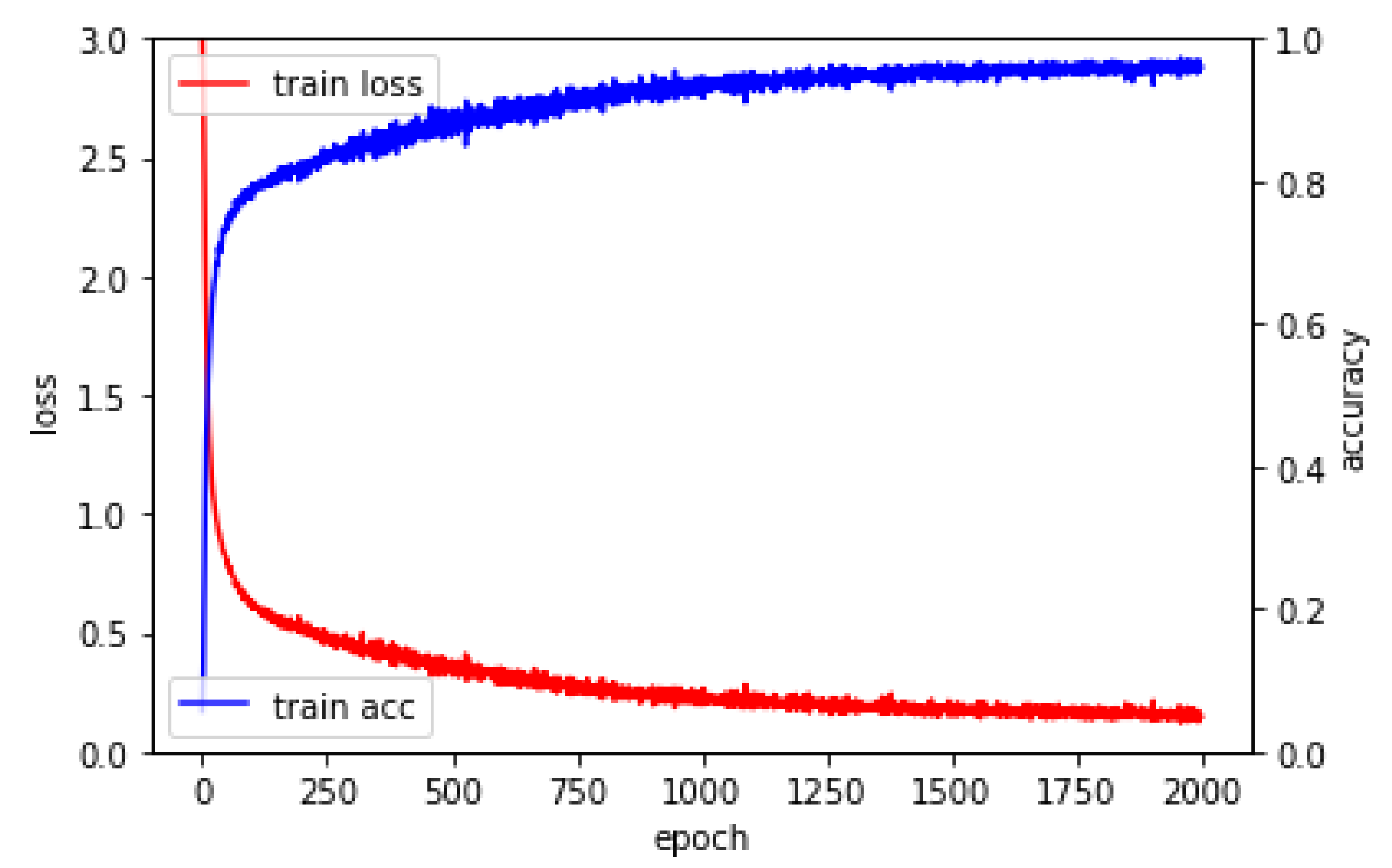
Finally, model fitting is required to execute the model. The training process will run for a fixed number of iterations over the dataset called epochs. The number of dataset rows is also arranged before the model weights are updated within each epoch, called the batch size. The number of epochs means the number of times that the algorithm repeatedly learns the entire training dataset. One epoch means that each sample of the training dataset can be used to update internal model parameters. The size of epochs is usually large up to hundreds to thousands to minimize errors sufficiently. The batch size is the number of samples processed before the model is updated. The numbers of epochs and batch sizes can be determined experimentally through trial and error. The model must be sufficiently trained to well map the rows of input data to the output classification. There are always some errors in the model, but after a certain point in time for a given model configuration, the model converges, and the amount of error is reduced. In this study, 2000 epochs and 200 batch sizes were used. Figure 5 shows the learning process of the neural network. Loss is a sum of errors that occurred for each example in the training set. Loss values indicate how well a particular model works after each optimization iteration. Ideally, the loss is expected to decrease after each or multiple iterations. The accuracy of the model is usually determined after training and correction of model parameters. The test sample is then provided to the model and compared to the actual target, and the number of times that the model makes a mistake is memorized.

Figure 5. Learning process of the network model.

4. Results and Discussions

4.1. Failure Identification Examples

While the mooring-failure-detection algorithm is designed, finding appropriate measurement parameters is the first important task to provide high-accuracy detection. Using the tension sensor is the most direct method to detect the failure. However, it is unrealistic to install the tension sensor to all mooring lines because tension sensors need regular calibrations and are hard to be repaired and replaced especially for deeply submerged structures such as SFT. In this regard, accelerometers, which can easily be installed inside the tunnel along its longitudinal direction, are chosen. Furthermore, it can be directly connected to the electric wire to continuously function in real time. Being inside in dry space, it is easy to be calibrated and checked up. For the present monitoring algorithm, we directly use the lateral and vertical displacements of SFT, which can be obtained by integrating the acceleration signals twice. We confirmed that appropriate bandwidth filter and baseline correction can accurately recover the displacements from accelerations during time integrations even if there is noise. Zheng et al. [33] showed the feasibility of real-time displacement monitoring using double integration of acceleration with measurement noise based on a recursive baseline correction and recursive high-pass filter. However, when mean displacements cannot be captured and/or noise cannot be handled during time integrations, real-time displacements can alternatively be obtained from inclinometers instead of accelerometers, as developed by 3rd author’s research group [34].

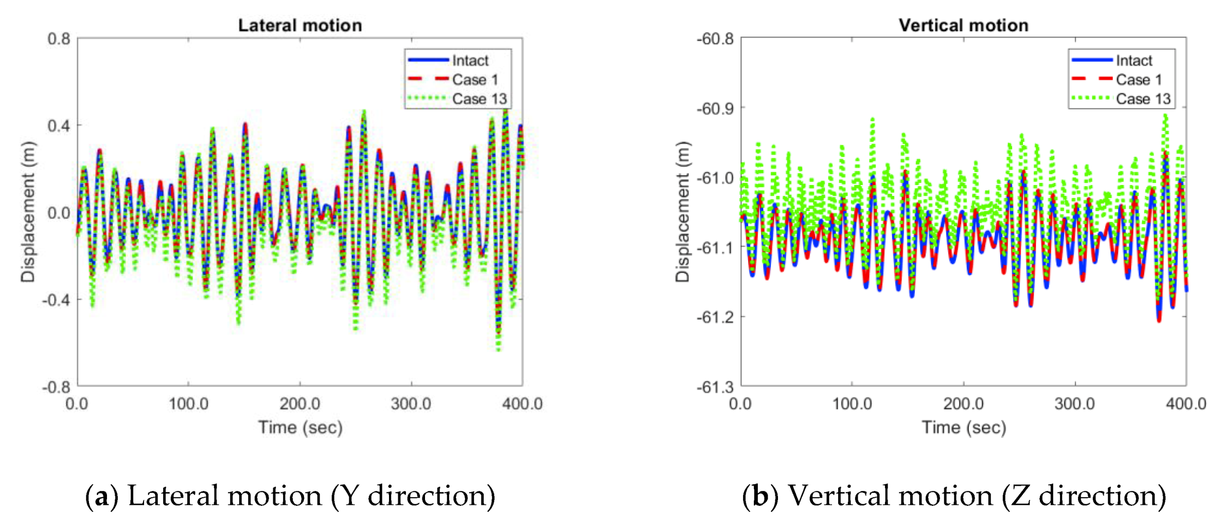
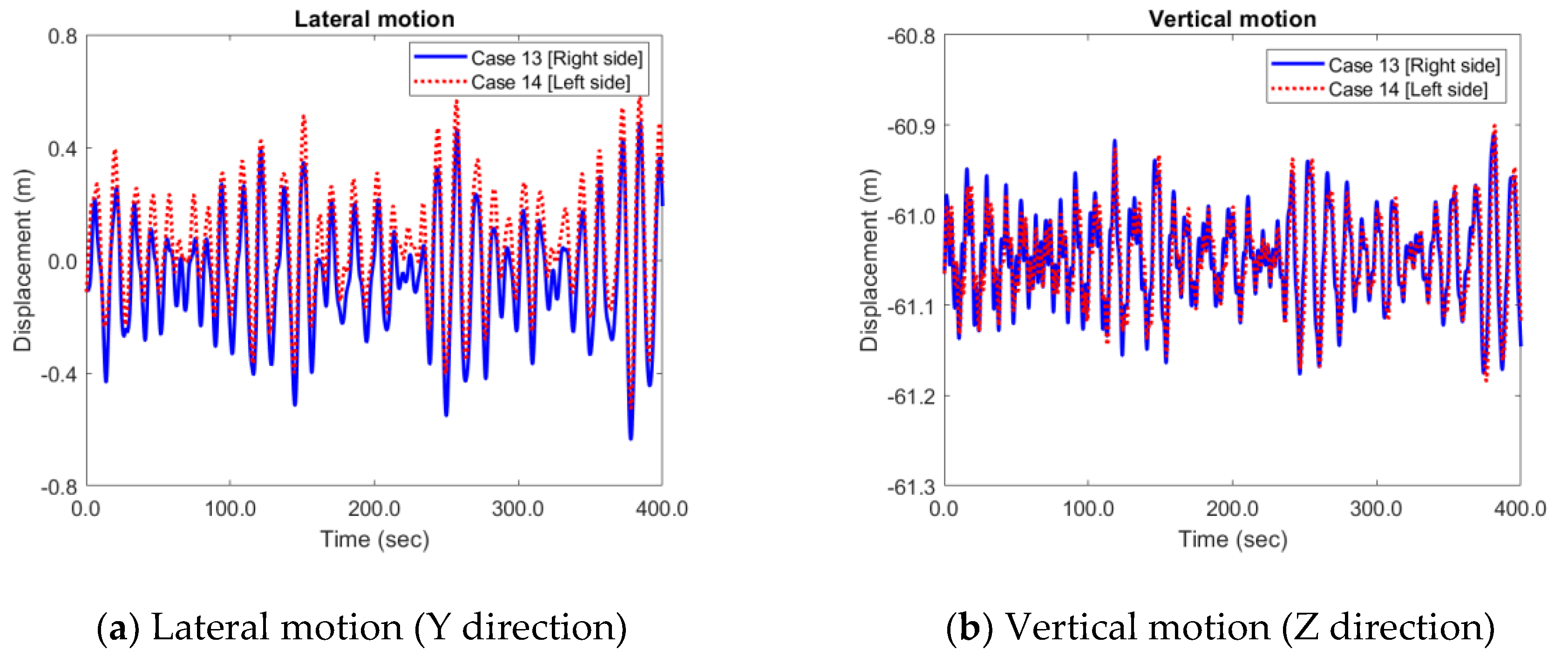
Figure 6 and Figure 7 show the time histories of lateral and vertical displacements of the tunnel at its mid-length (sensor No. 5, x = 0 m) in intact and failure scenarios. While simulation time is 1800 sec (9000 steps), the results for the first 400 sec are presented there. The corresponding significant wave height and peak period are 11.7 m and 13 sec. Cases 1 and 13 in Figure 6 are the results when one of the mooring lines is broken at x = −300 m and x = 0 m, respectively (see Table 2). There are noticeable differences between the intact case and Case 13. For the lateral motion, Case 13 has lager motions in the negative direction since one-mooring failure leads to less stiffness of the system there. The larger fluctuations and static shift of the vertical displacement are observed for Case 13. These results demonstrate that failure can more easily be detected by motion changes when sensors are close to the failure locations. On the other hand, for Case 1, since the failure location (x = - 300 m) is far away from the sensor location (x = 0 m), there is no visible difference in displacements between intact and failure cases. In addition, as shown in Figure 7, depending on the left- and right-side mooring failure, the corresponding asymmetrical bias can be observed in the lateral motion trends. However, the corresponding difference in the vertical response is small, as can be seen from Figure 7b. By observing the pattern of those sensor signals, the monitoring algorithm can figure out the best guess for the failure incidence. If we place several accelerometers along the longitudinal direction of the tunnel, the prediction accuracy can significantly be improved while much more detailed comparisons of multiple sensor signals have to be made. As was seen in Figure 7, two-directional (horizontal and vertical) signals will be beneficial to better classify the failure location.

Figure 6. Time histories of lateral and vertical displacements of the tunnel at its mid-length (sensor No. 5) in intact and failure conditions.

Figure 7. Time histories of lateral and vertical displacements of the tunnel at its mid-length (numerical sensor No. 5) in two different mooring-failures in the opposite sides.

4.2. Optimization

4.2.1. Hidden Layer and Neuron

Several optimizations are processed before evaluating the performance of the machine-learning algorithm. The optimized parameters are determined based on the accuracy and loss function defined in Section 3. Accuracy is a way to measure the performance of a classification model. The higher the accuracy, the better the algorithm. The accuracy of the perfect failure-detection algorithm is 1. On the other hand, the loss function considers the probability or uncertainty of the prediction depending on how different the prediction is from the actual value. The loss is the sum of the errors that occurred for each sample in the training. The perfect failure-detection algorithm has zero loss.

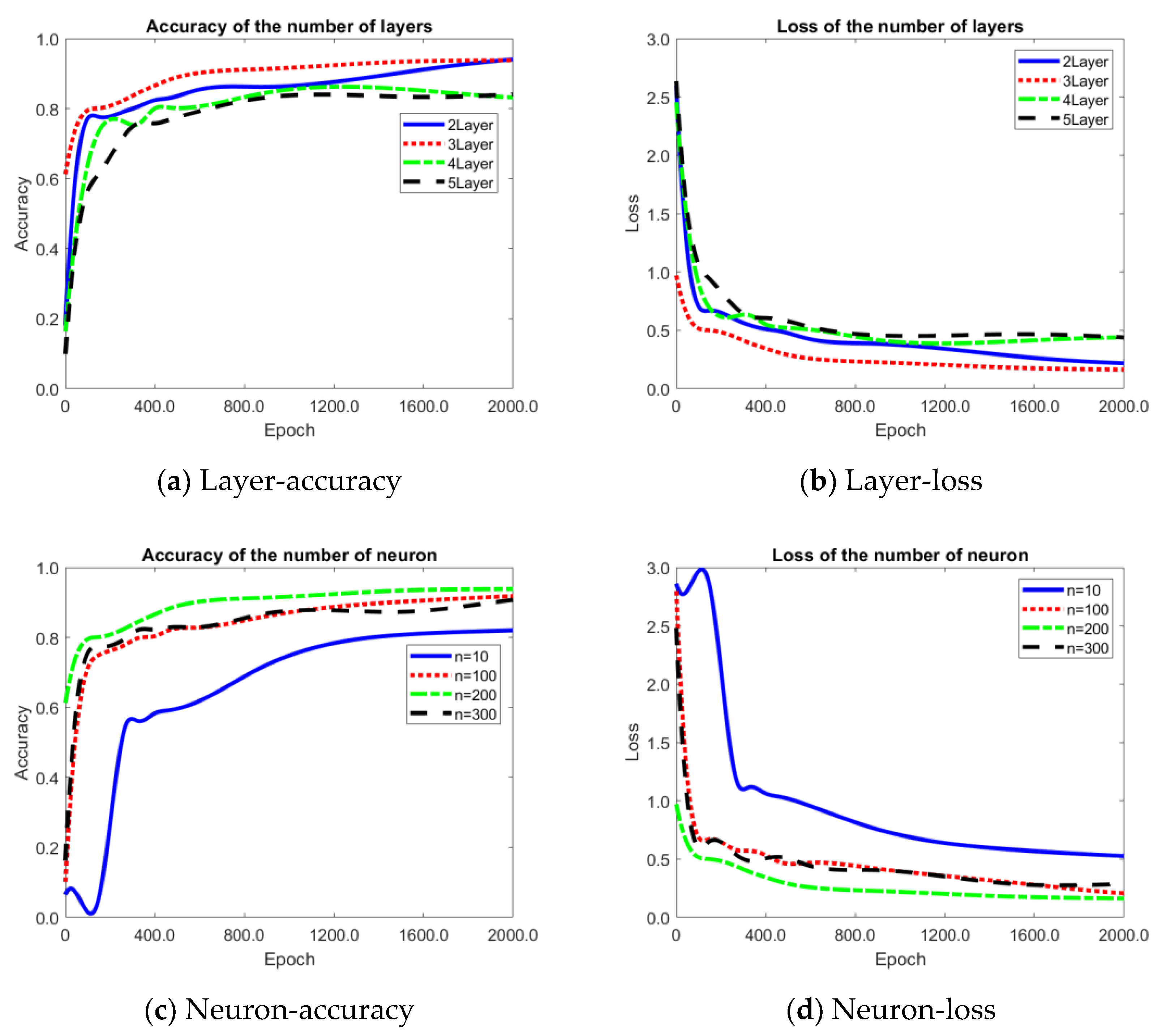
The performance tests are firstly conducted with respect to the numbers of the hidden layers and neurons in each layer. Generally, ANN cannot analytically determine the best numbers of layers and neurons of each layer. In addition, using a single hidden layer makes it difficult to express the relationship between inputs and outputs since they are linearly linked. Therefore, the number of hidden layers and neurons should be optimized through the performance tests, as presented in Figure 8. In the optimization process, we utilized the signals from seven sensors (#2–8) that are equally spaced. The algorithm randomly selects 80% of the entire dataset for training from the first eight environmental conditions given in Table 3 and uses the remaining 20% of the dataset to check the accuracy and loss. While the epoch increases from 1 to 2000, accuracy and loss are evaluated. These procedures are also adopted in the next optimization process. As shown in Figure 8, the highest accuracy and lowest loss can be acquired with three hidden layers and 200 neurons, and these values are used in the ensuing study. In general, the higher the epoch, the higher the accuracy. Interestingly, increasing the hidden layers and neurons more than three and 200 does not provide higher accuracy.

Figure 8. Performance test for the number of hyperparameters.

4.2.2. Activation Function and Optimizer

Next, the activation function and optimizer are to be selected through this optimization process. Sigmoid, Tanh, ReLU, and SELU are compared for the activation-function optimization while RMSProp, AdaGrad, Adam, and Adamax are compared for the optimizer performance. Their characteristics and advantages/disadvantages are summarized in Table 4 [25,26,27,28,29,30,31,32].

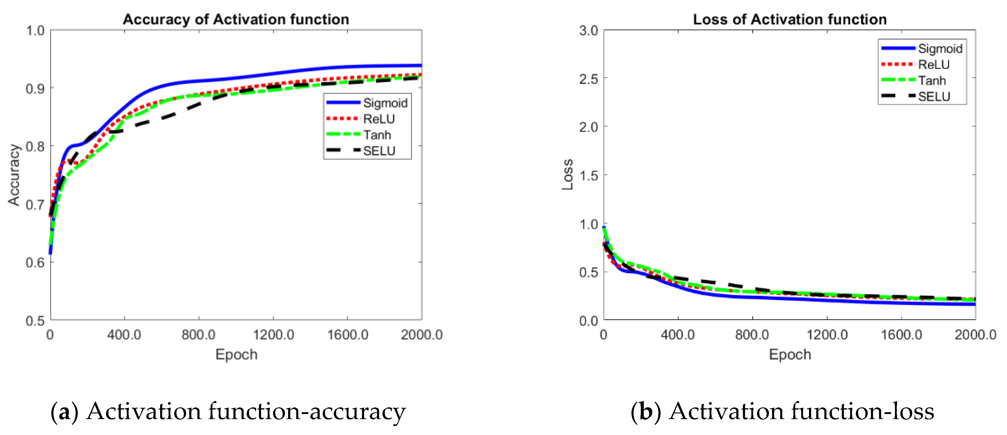
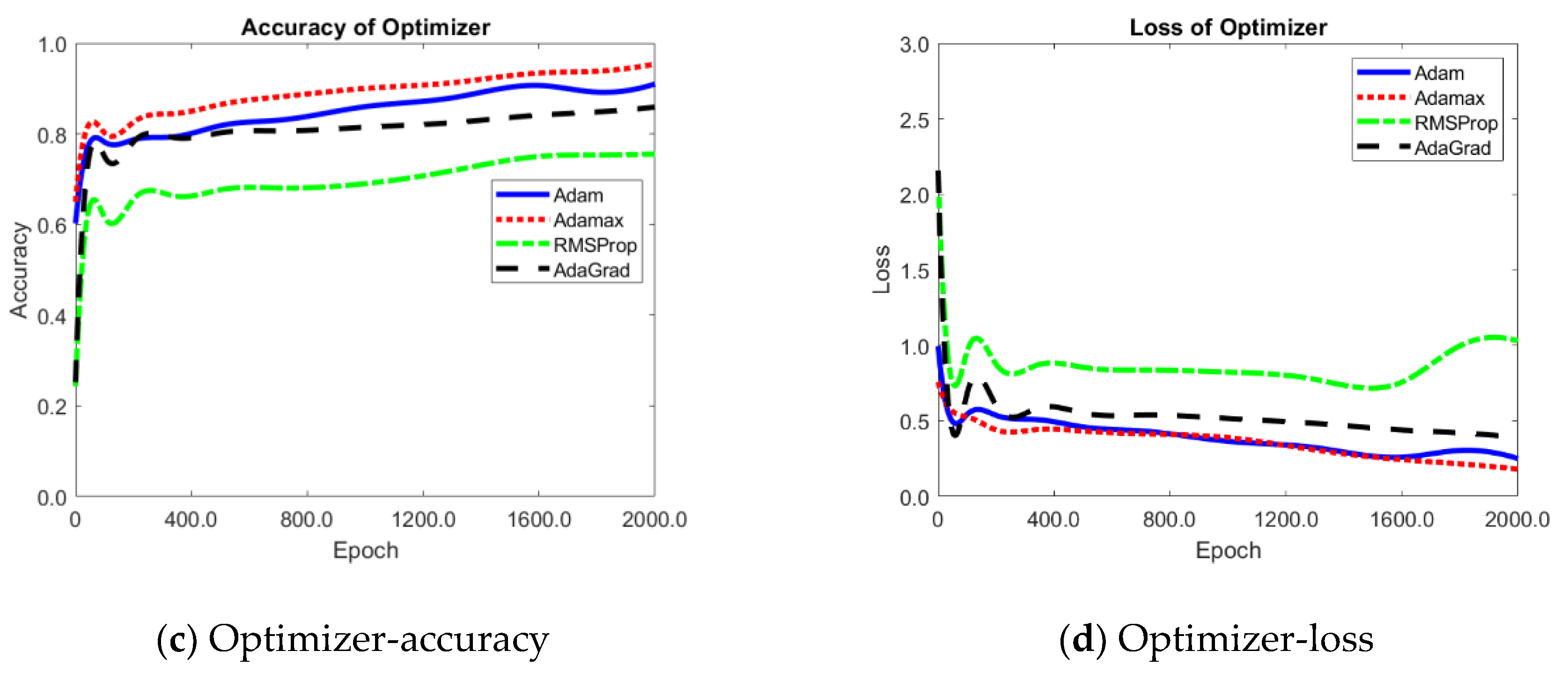
As shown in Figure 9, the Sigmoid function, one of the most classic activation function, provides the best results than any other activation functions. This indicates that the Sigmoid function operates nicely as a classifier for the present goal. As for optimizer, Adamax outperforms other optimizers. In this regard, Sigmoid and Adamax are selected as the activation function and optimizer.

Figure 9. Performance test for the selection of the activation function and optimizer.

4.3. Failure-Detection Performance

Based on the previous optimization results, the numbers of hidden layers and neurons are three and 200, and the selected activation function and optimizer are Sigmoid and Adamax, respectively. The epoch is set as 2000. These parameters and functions are further utilized to check the failure-detection accuracy of the present algorithm. Again, the algorithm randomly selects 80% of the entire dataset for training from the first eight environmental conditions given in Table 3 and uses the remaining 20% of the dataset for testing by checking the corresponding accuracy and loss.

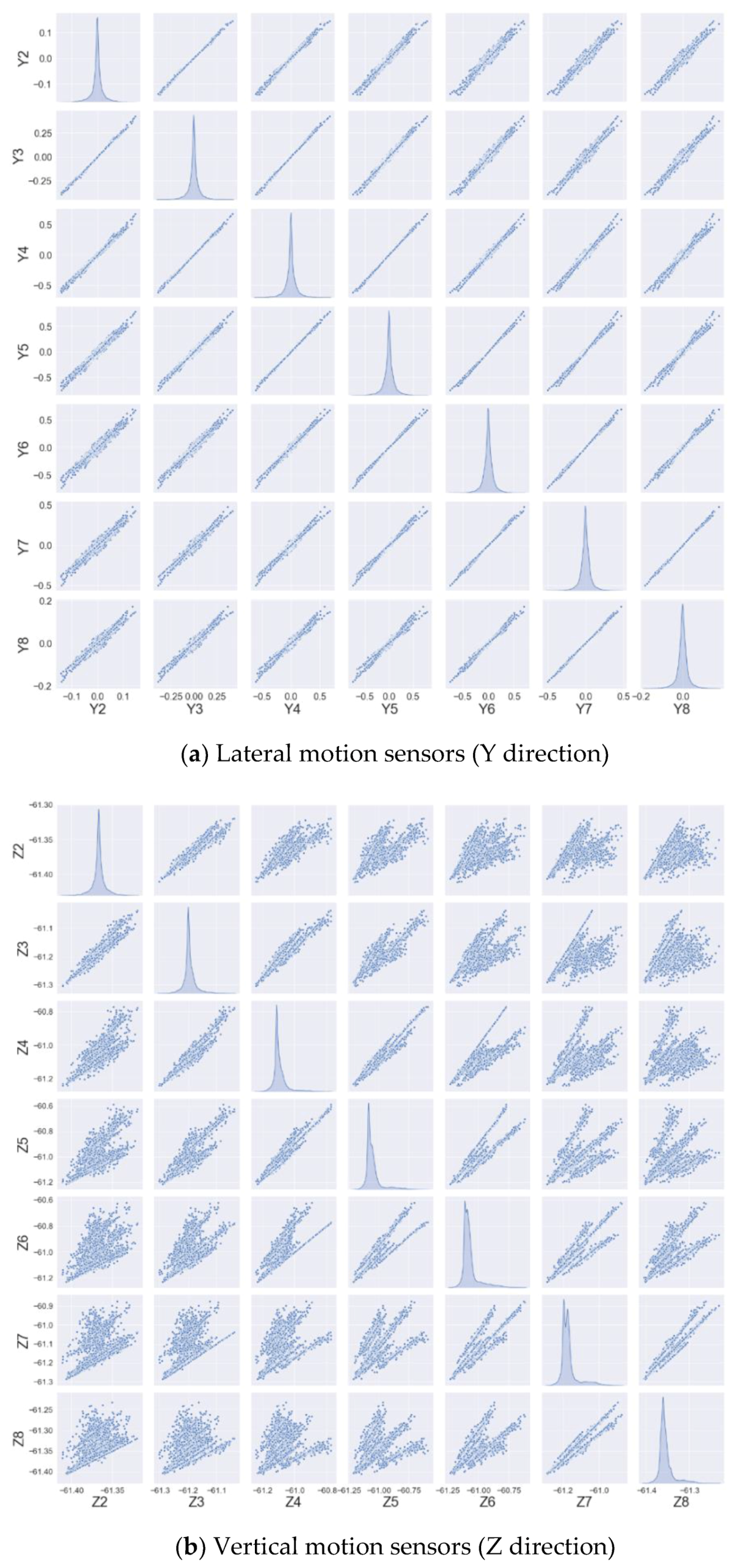
Figure 10 shows the correlation between numerical sensors for lateral and vertical motions. Correlation analysis is a technique that analyzes the linear relationship between two variables measured continuously. For example, in Figure 10a, the figure in the first row and the second column shows the relationship between the sensor No. 2 and sensor No. 3 (see Figure 1 for sensor numbers). We can see their strong relationship since the figure looks like a very slender ellipse along the diagonal. For the combination of first row and last column representing sensors 2 and 8, a less strong relationship can be observed with a wider ellipse. In other words, the longer the distance between the sensors, the less the correlation. The relationship is less strong in vertical displacements under different failure scenarios since vertical motions are smaller having 60-degree mooring toe angle and relatively large BWR (=1.3), and thus less sensitive to certain mooring-line failure. If the BWR is decreased, the vertical displacements are increased [7,17], then they are to play a more important role. As a result, the distance between sensors should be short enough to acquire high detection accuracy but large enough to minimize cost and complexity. Therefore, the optimization of the sensor interval and number in real monitoring applications is important.

Figure 10. Correlation of numerical sensor data for lateral (a) and vertical (b) motions.

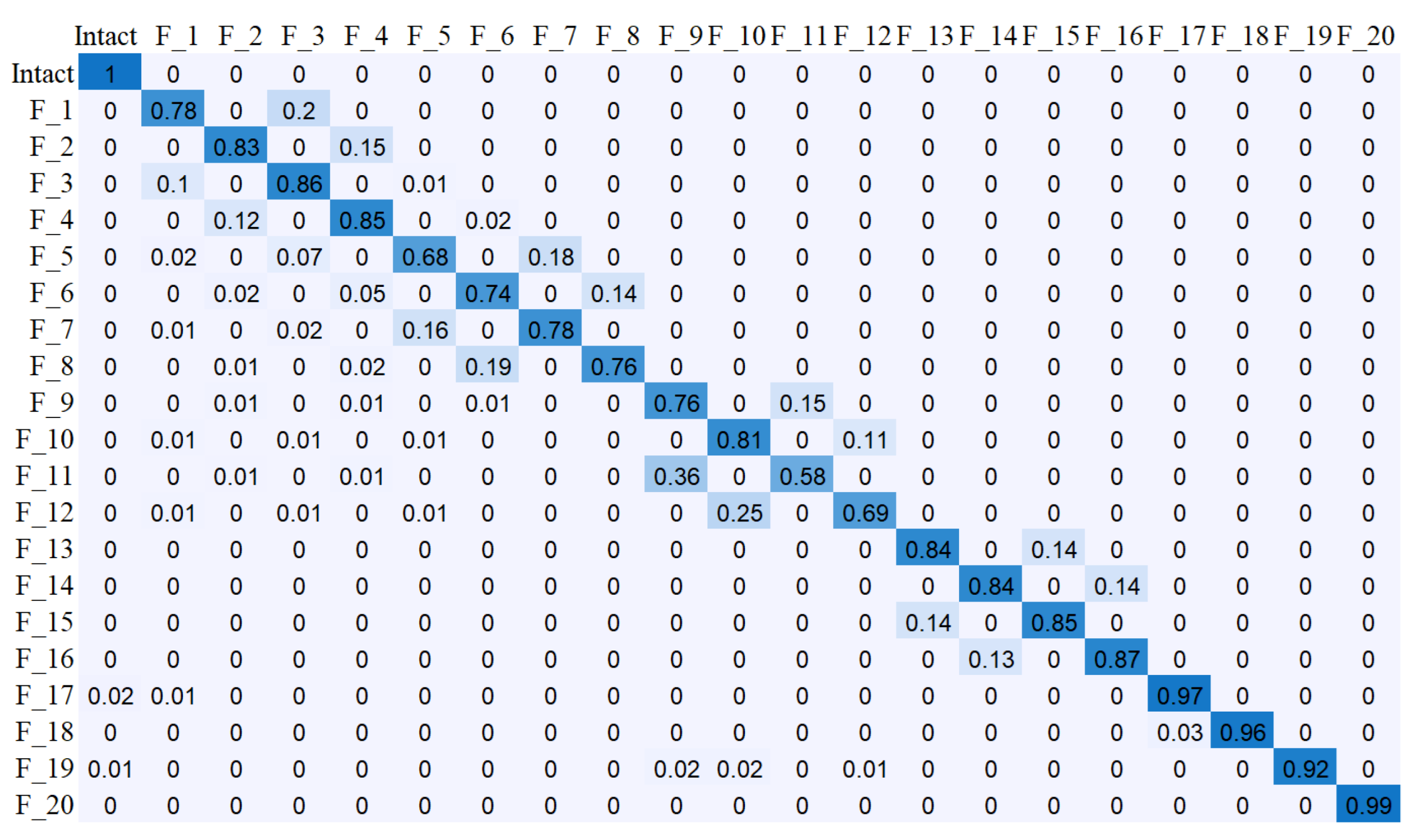
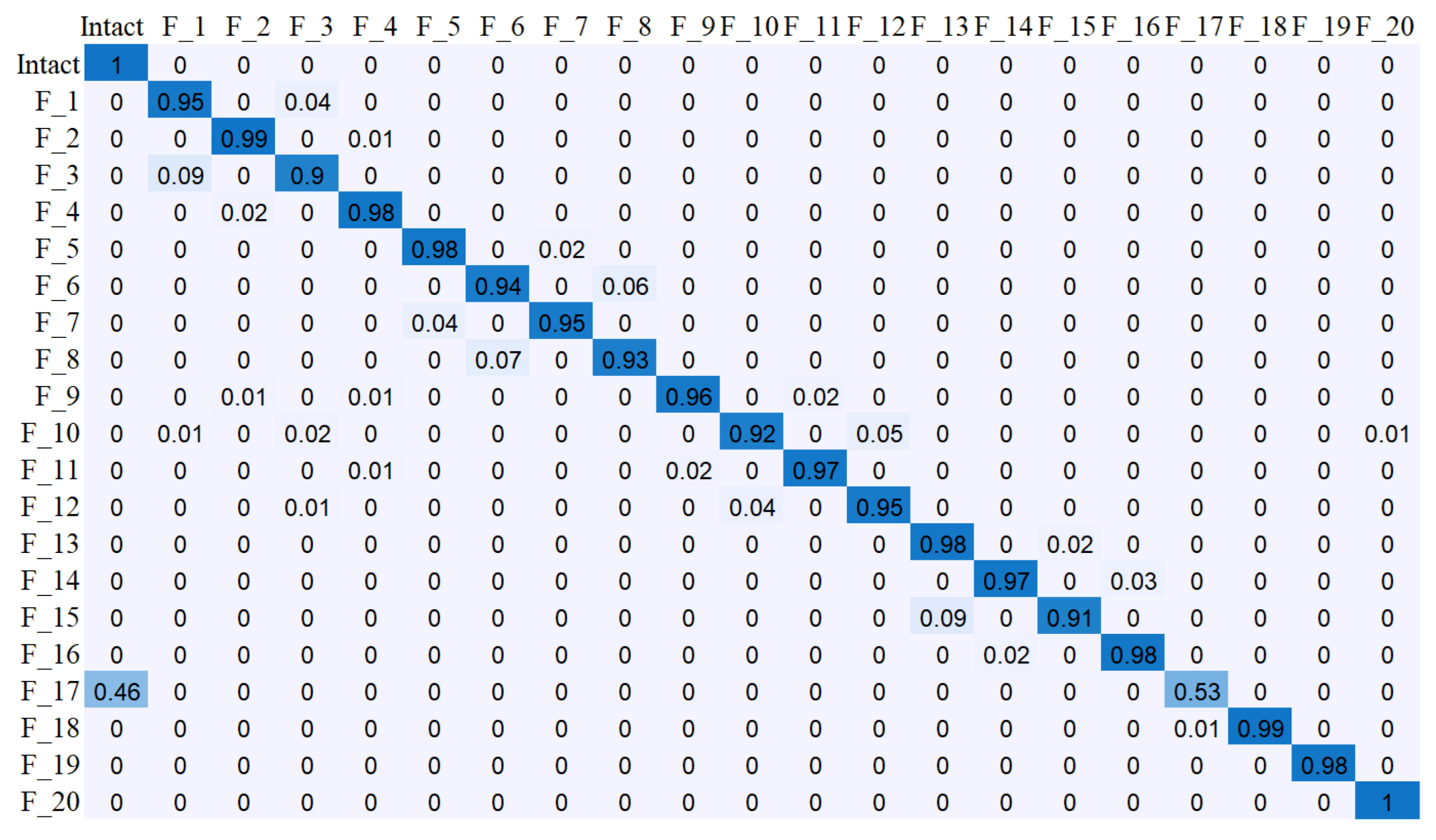
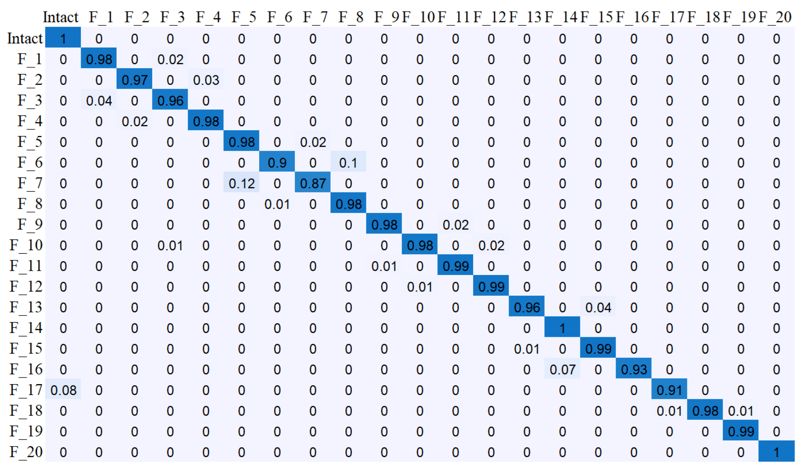
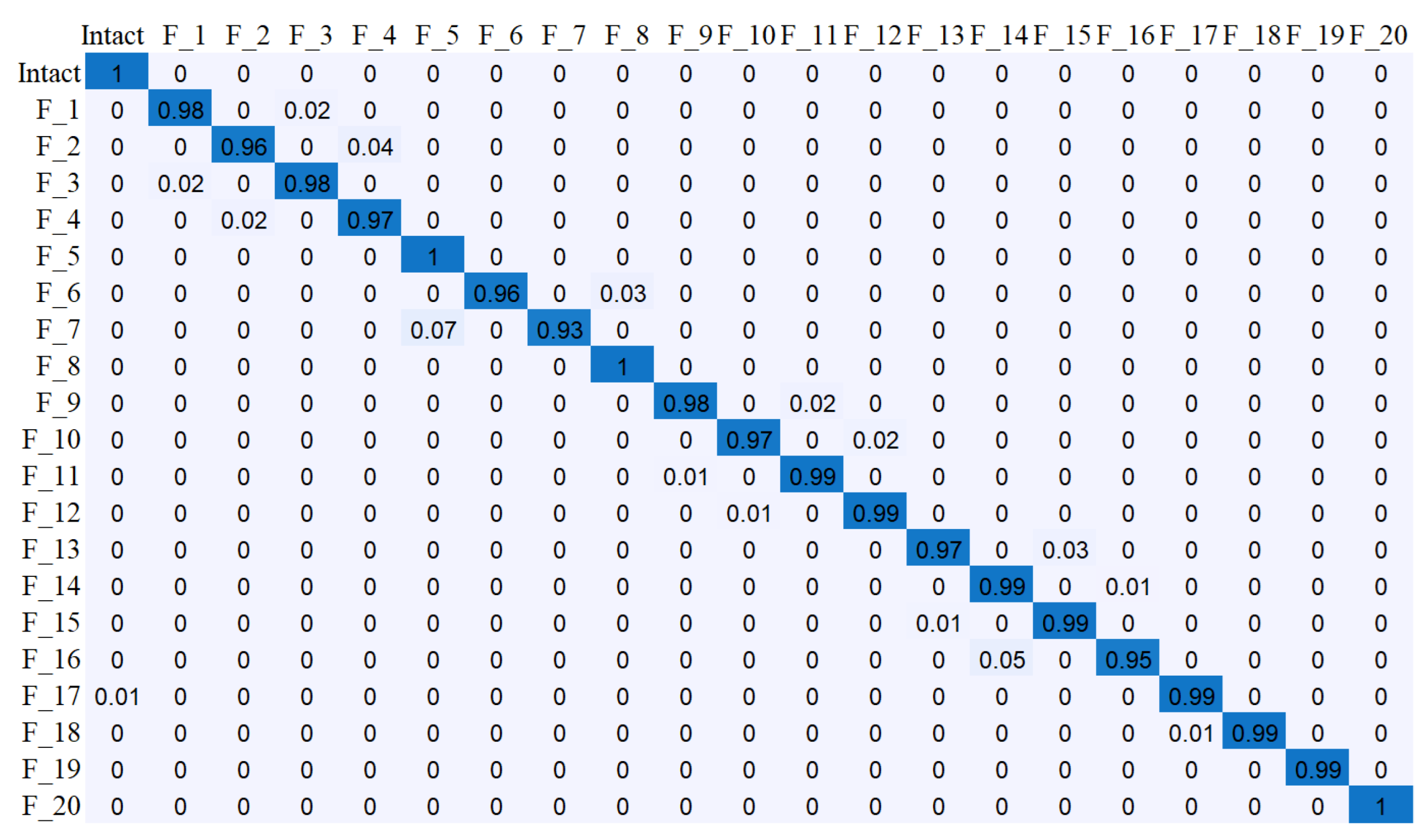
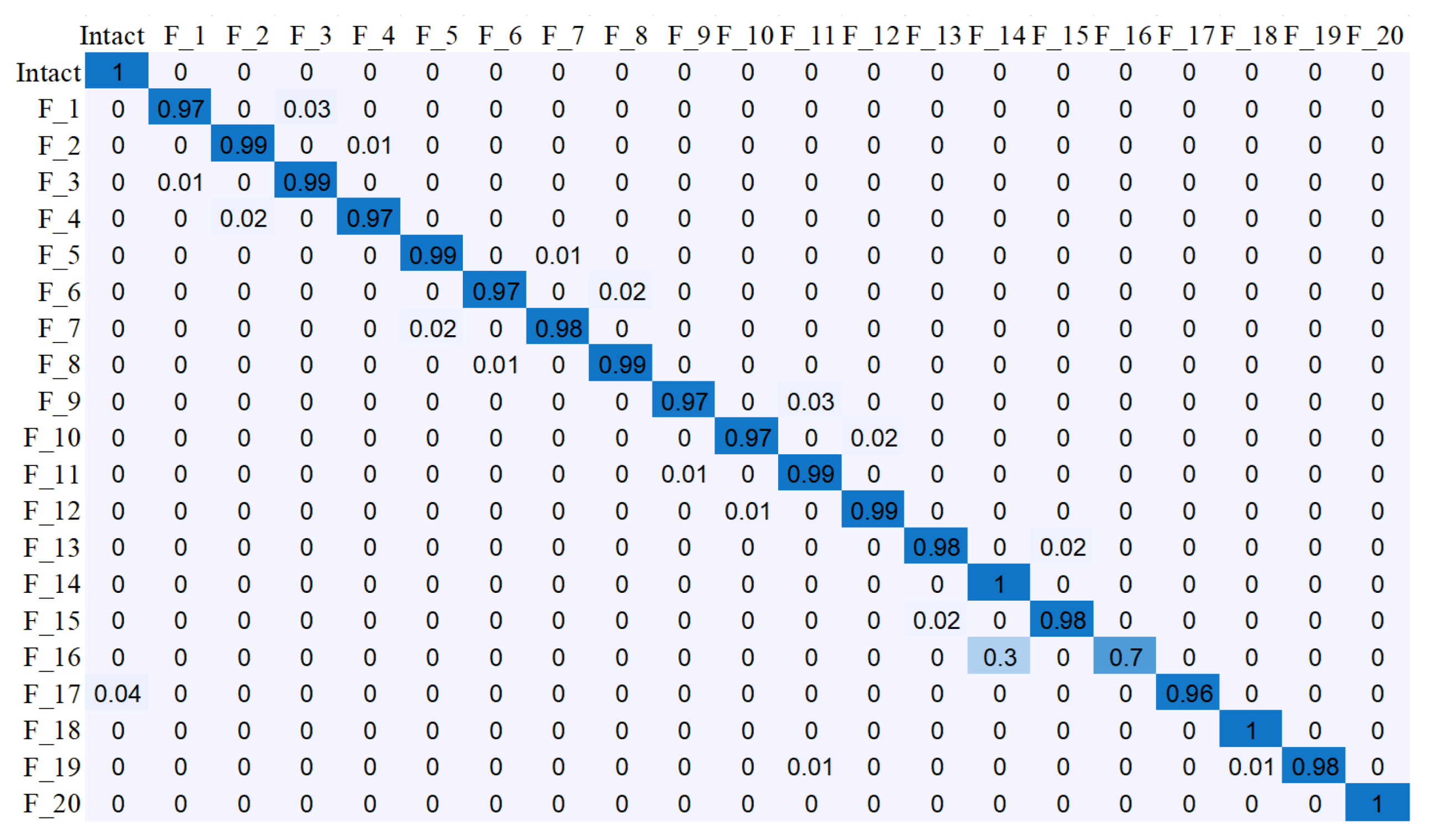
Figure 11, Figure 12, Figure 13, Figure 14, Figure 15 and Figure 16 show the confusion matrices at different sensor combinations. The confusion matrix represents the performance of the classifier in a series of test data of which actual values are known [35]. The confusion matrices are a good option for reporting the performance results in multi-class classification problems because it is possible to observe the relations between the classifier outputs and the true ones. Table 5 summarizes the accuracy of classification with different numbers of sensors. The elements n_ij in the confusion matrix, where i and j are row and column identifiers, indicate the cases belonging to i that is classified as j. Hence, the elements in the diagonal (n_ii) are the elements correctly classified, while the off-diagonal elements in the matrix are misclassified. The total number of cases is expressed as:

$$N={\displaystyle \sum _{i=1}^M{\displaystyle \sum _{j=1}^M{n}_{ij}}}$$

(6)

where M is the number of failure/intact scenarios. The confusion matrices show the ratio of detected cases to total cases in a range [0,1]. An asymmetric confusion matrix can reveal a biased classifier. The accuracy is the probability of performing the correct classification. The accuracy can be calculated from the confusion matrix as:

$$\mathrm{Accuracy}=\frac{{\displaystyle \sum _{i=1}^M{n}_{ii}}}{N}$$

(7)

Figure 11. Failure detected location when there are 3 sensors at points 2, 5, and 8 (Accuracy: 84.1%).

Figure 12. Failure detected location when there are 4 sensors at points 2, 4, 6, and 8 (Accuracy: 90.4%).

Figure 13. Failure detected location when there are 5 sensors at points 3, 4, 5, 6, and 7 (Accuracy: 92.9%).

Figure 14. Failure detected location when there are 5 sensors at points 2, 3, 5, 7, and 8 (Accuracy: 94.2%).

Figure 15. Failure detected location when there are 5 sensors at points 2, 4, 5, 6, and 8 (Accuracy: 96.7%).

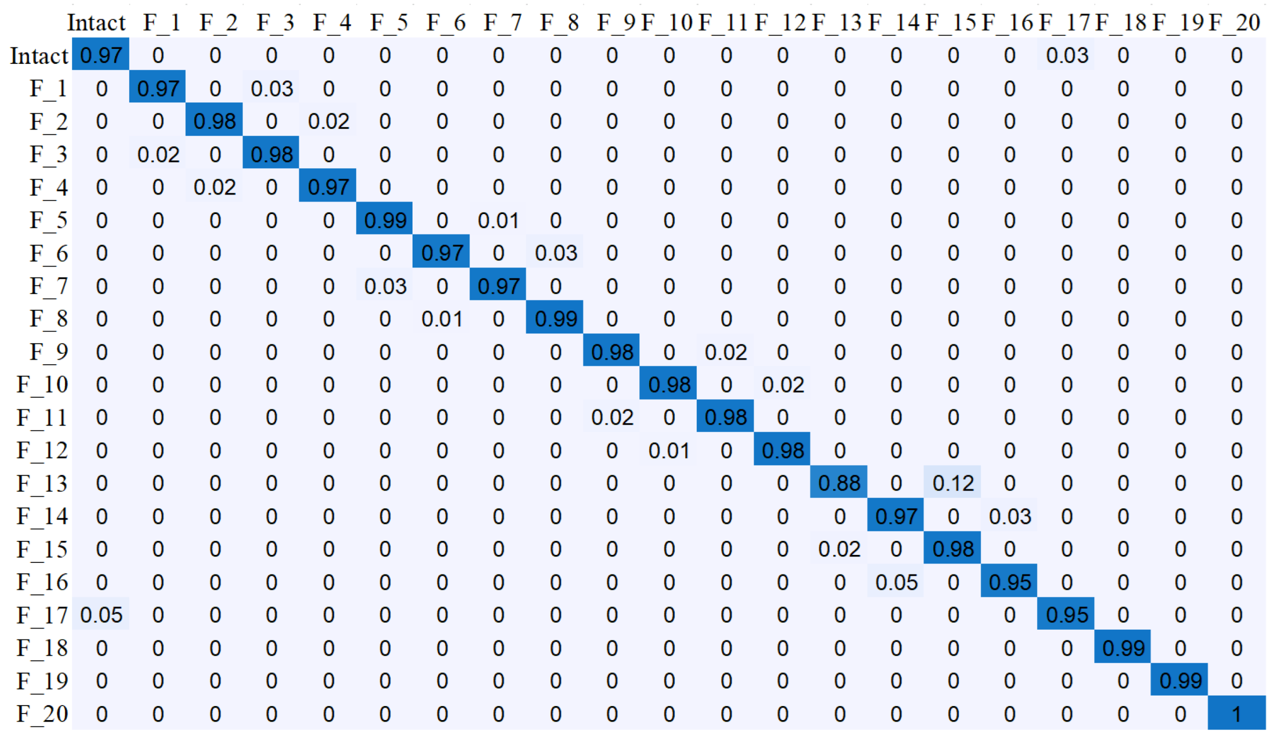
Figure 16. Failure detected location when there are 7 sensors at points 2, 3, 4, 5, 6, 7, and 8 (Accuracy: 98.1%).

Table 5. Failure-detection accuracy at different sensor combinations.

	Sensor Location
	2, 5, 8	2, 4, 6, 8	3, 4, 5, 6, 7	2, 3, 5, 7, 8	2, 4, 5, 6, 8	2, 3, 4, 5, 6, 7, 8
Accuracy (%)	84.1	90.4	92.9	94.2	96.7	98.1

Here, we set a rule; if the classification probability of a certain failure case is less than 50%, there is no classification at each time step. For instance, at nth time step, the probabilities of Case 3 and Case 5 are 42.6% and 45.0%, respectively, then, they are regarded as no classification. Base on this rule, the summation of values is less than 1 in several rows in Figure 11, Figure 12, Figure 13, Figure 14, Figure 15 and Figure 16.

As shown in Figure 11, with three sensors (No. 2, 5, and 8), the overall classification accuracy is low (84.1% accurate), except for the intact case and cases when all mooring lines are broken i.e., Cases 17–20. Mostly, misclassification occurs when the adjacent mooring is broken, but, the probability of correct classification is always higher than that of misclassification, even if the classification was not good enough. Figure 12 shows the results with four sensors (No. 2, 4, 6, and 8). After adding one more sensor, the overall classification accuracy is increased to 90.4% i.e., failure detection performance is significantly enhanced. However, there are some scenarios where accuracy is lower than the three-sensor case, which supports the necessity of sensor-location optimization. We can further check the importance of sensor arrangement in the longitudinal direction, as shown in Figure 13, Figure 14 and Figure 15. With the same sensor number of five, quite different detection accuracies can be obtained. Widely spread sensors (Figure 14 and Figure 15) provide higher accuracy than centrally packed sensors (Figure 13). When comparing Figure 14 with Figure 15, a sufficient number of sensors should be located near central locations where the largest motion variations occur as a result of different mooring failures. Placing three sensors in the central areas (Figure 15) results in higher detection accuracy than the case with one sensor in the center (Figure 14). Finally, as shown in Figure 16, with seven sensors, the highest detection accuracy of 98.1% is obtained. Small misclassifications recognizing the mooring-failure case of F7 as F5 occurred, but their failure locations were the same i.e., x = −200 m. Judging from the trend, with more sensors, the mooring failure prediction can be even higher than 98.1%. The improvement from Figure 15 with five sensors (96.7%) to Figure 16 with 7 sensors (98.1%) is only marginal. Therefore, when 97% prediction accuracy is good enough, we can install five sensors instead of seven sensors to lower the relevant cost and complexity. Even lower failure-prediction accuracy than 97% may still be acceptable since with the warning sign, we can always double-check the actual failure by sending divers or underwater drones.

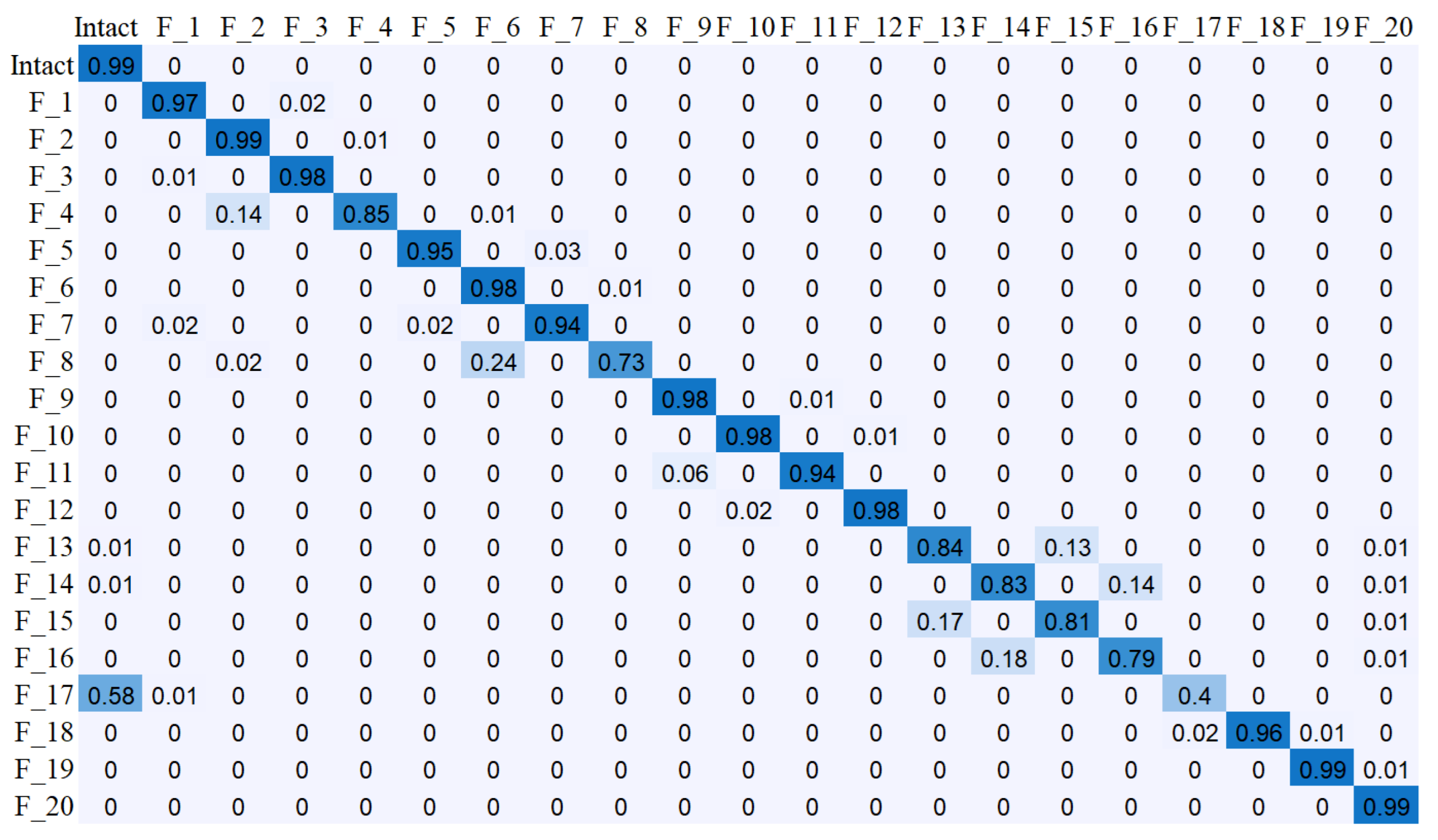
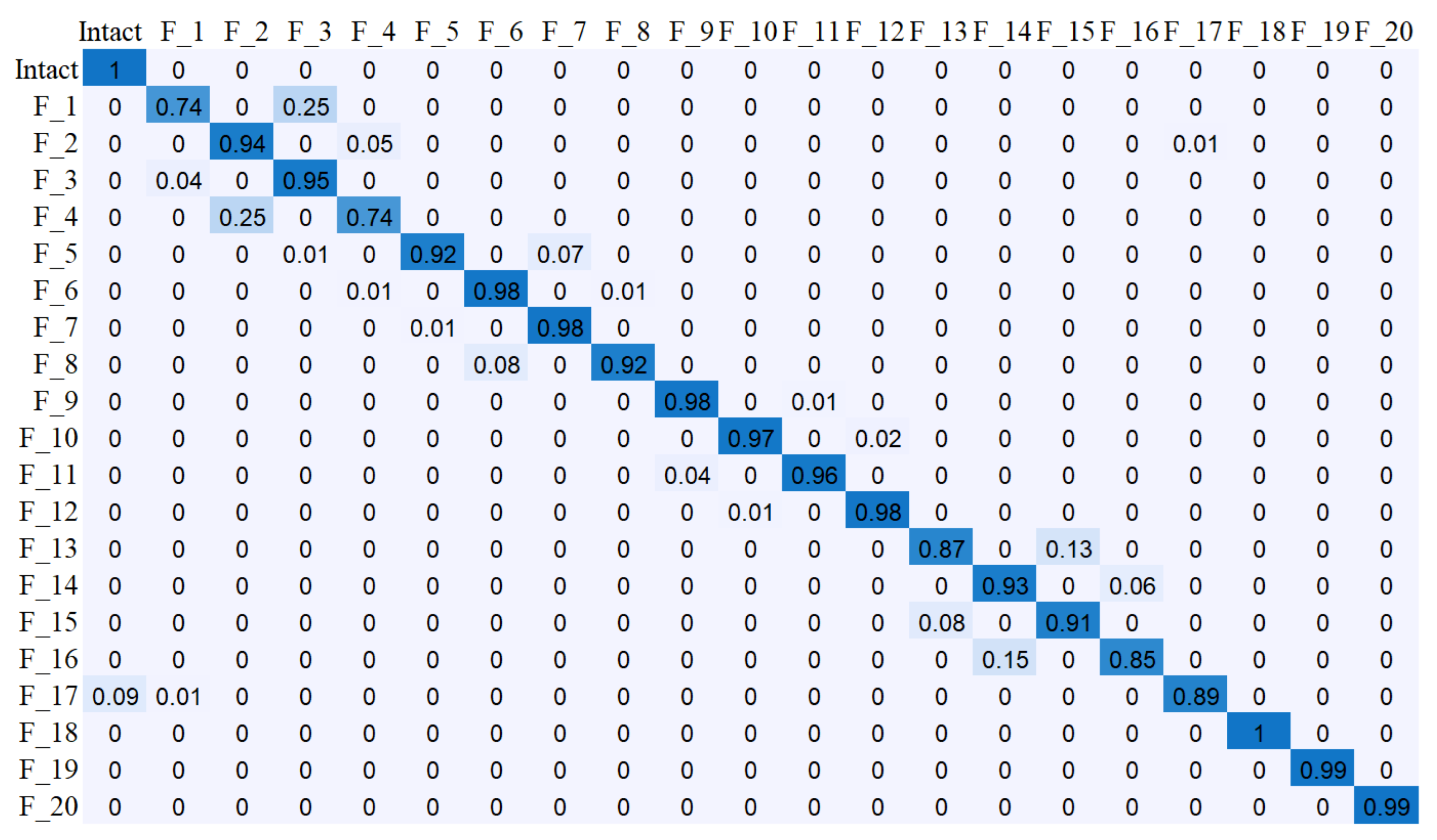
In order to further verify model accuracy in various marine environments, two more wave conditions (Hs = 3 m, Tp = 8 sec; Hs = 7 m, Tp = 12 sec, i.e., the last two environmental conditions given in Table 3) were considered for testing to evaluate the failure detection performance, which was not considered in training. Same as the previous cases, 80% of the dataset from the first eight environmental conditions were used as a training set, and the data from seven sensors (#2–8) that showed the best performance were used. As shown in Figure 17 and Figure 18, the results show that even if different environmental conditions were tested, sufficient accuracy of over 97% was obtained. Therefore, the reliability of the model is secured by showing very high accuracy even for the environmental conditions not used as training data.

Figure 17. Confusion matrix of the different environmental condition (Hs = 3 m, Tp = 8 sec) (Accuracy: 97.0%).

Figure 18. Confusion matrix of the different environmental condition (Hs = 7 m, Tp = 12 sec) (Accuracy: 97.2%).

5. Conclusions

This paper presents the development of a DNN (deep neural network) model for detecting and classifying mooring-failure locations for SFT using lateral and vertical motion-sensor signals. This task can be considered as pattern-recognition and classification problems, and DNN is appropriate for the task. The input variables of the algorithm are sea state (Hs and Tp) and lateral and vertical displacement data from three to seven sensors. The hydro-elastic tunnel-mooring coupled time-domain simulations were performed under different wave conditions and failure/intact scenarios, and the big dataset of numerical-sensor signals was acquired. Through simulations, we confirmed that trends and magnitudes of displacements were changed under different failure (or intact) scenarios. The entire data set basically consists of 80% training data and 20% test data not used for training from eight wave conditions. Two wave conditions not used for training were additionally employed for further testing. The optimization process was progressively conducted with respect to the numbers of hidden layers and neurons of each layer, activation function, and optimizer. The selected optimal numbers of hidden layers and neurons were three and 200, respectively. The Sigmoid activation function and Adamax optimizer were selected for high classification accuracy. We also tested the failure-detection performance with different numbers and combinations of motion sensors. Misclassification largely decreases as the number of sensors is increased with proper intervals. With seven motion sensors, the classification accuracy of 98.1% was achieved. The prediction accuracy higher than 90% can also be achieved even with four sensors. Besides, the model displays the accuracy of over 97% with the different wave conditions that were not used in the training data set. The results show good feasibility of the developed machine-learning-based monitoring system for the mooring-failure detection of future SFTs or similar deformable submerged structures.

References

- di Pilato, M.; Perotti, F.; Fogazzi, P. 3D dynamic response of submerged floating tunnels under seismic and hydrodynamic excitation. Eng. Struct. 2008, 30, 268–281. [Google Scholar] [CrossRef]
- Faggiano, B.; Landolfo, R.; Mazzolani, F. The SFT: An innovative solution for waterway strait crossings. In IABSE Symposium Report; International Association for Bridge and Structural Engineering: Lisbon, Portugal, 2005; Volume 90, pp. 36–42. [Google Scholar]
- Seo, S.-I.; Mun, H.-S.; Lee, J.-H.; Kim, J.-H. Simplified analysis for estimation of the behavior of a submerged floating tunnel in waves and experimental verification. Marine Struct. 2015, 44, 142–158. [Google Scholar] [CrossRef]
- Chen, Z.; Xiang, Y.; Lin, H.; Yang, Y. Coupled vibration analysis of submerged floating tunnel system in wave and current. Appl. Sci. 2018, 8, 1311. [Google Scholar] [CrossRef]
- Long, X.; Ge, F.; Hong, Y. Feasibility study on buoyancy–weight ratios of a submerged floating tunnel prototype subjected to hydrodynamic loads. Acta Mech. Sin. 2015, 31, 750–761. [Google Scholar] [CrossRef]
- Lu, W.; Ge, F.; Wang, L.; Wu, X.; Hong, Y. On the slack phenomena and snap force in tethers of submerged floating tunnels under wave conditions. Marine Struct. 2011, 24, 358–376. [Google Scholar] [CrossRef]
- Jin, C.; Kim, M.-H. Time-domain hydro-elastic analysis of a SFT (submerged floating tunnel) with mooring lines under extreme wave and seismic excitations. Appl. Sci. 2018, 8, 2386. [Google Scholar] [CrossRef]
- Won, D.; Seo, J.; Kim, S.; Park, W.-S. Hydrodynamic Behavior of Submerged Floating Tunnels with Suspension Cables and Towers under Irregular Waves. Appl. Sci. 2019, 9, 5494. [Google Scholar] [CrossRef]
- Ma, Z.; Sohn, H. Structural Displacement Estimation by FIR Filter Based Fusion of Strain and Acceleration Measurements. In Proceedings of the 29th International Ocean. and Polar Engineering Conference, Honolulu, HI, USA, 16–21 June 2019; International Society of Offshore and Polar Engineers: Cupertino, CA, USA, 2019. [Google Scholar]
- Choi, J.; Kim, J.M.-H. Development of a New Methodology for Riser Deformed Shape Prediction/Monitoring. In Proceedings of the ASME 2018 37th International Conference on Ocean., Offshore and Arctic Engineering, Madrid, Spain, 17–22 June 2018; American Society of Mechanical Engineers Digital Collection: New York, NY, USA, 2018. [Google Scholar]
- Mercan, B.; Chandra, Y.; Maheshwari, H.; Campbell, M. Comparison of Riser Fatigue Methodologies Based on Measured Motion Data. In Proceedings of the Offshore Technology Conference, Houston, TX, USA, 2–5 May 2016; Offshore Technology Conference, Inc.: Houston, TX, USA, 2016. [Google Scholar]
- Chung, M.; Kim, S.; Lee, K.; Shin, D.H. Detection of damaged mooring line based on deep neural networks. Ocean Eng. 2020, 209, 107522. [Google Scholar] [CrossRef]
- Jaiswal, V.; Ruskin, A. Mooring Line Failure Detection Using Machine Learning. In Proceedings of the Offshore Technology Conference, Houston, TX, USA, 6–9 May 2019; Offshore Technology Conference, Inc.: Houston, TX, USA, 2019. [Google Scholar]
- Sidarta, D.E.; Lim, H.-J.; Kyoung, J.; Tcherniguin, N.; Lefebvre, T.; O’Sullivan, J. Detection of Mooring Line Failure of a Spread-Moored FPSO: Part 1—Development of an Artificial Neural Network Based Model. In Proceedings of the International Conference on Offshore Mechanics and Arctic Engineering, Glasgow, Scotland, UK, 9–14 June 2019; American Society of Mechanical Engineers: New York, NY, USA; Volume 58769, p. V001T01A042. [Google Scholar]
- Sidarta, D.E.; O’Sullivan, J.; Lim, H.-J. Damage detection of offshore platform mooring line using artificial neural network. In Proceedings of the International Conference on Offshore Mechanics and Arctic Engineering, Madrid, Spain, 17–22 June 2018; American Society of Mechanical Engineers: New York, NY, USA; Volume 51203, p. V001T01A058. [Google Scholar]
- Orcina. OrcaFlex Manual. Available online: https://www.orcina.com/SoftwareProducts/OrcaFlex/index.php (accessed on 17 October 2018).
- Jin, C.; Kim, M.-H. Tunnel-mooring-train coupled dynamic analysis for submerged floating tunnel under wave excitations. Appl. Ocean. Res. 2020, 94, 102008. [Google Scholar] [CrossRef]
- Cifuentes, C.; Kim, S.; Kim, M.; Park, W. Numerical simulation of the coupled dynamic response of a submerged floating tunnel with mooring lines in regular waves. Ocean Syst. Eng. 2015, 5, 109–123. [Google Scholar] [CrossRef]
- Kim, H.; Jin, C.; Kim, M.; Kim, K. Damage detection of bottom-set gillnet using Artificial Neural Network. Ocean Eng. 2020, 208, 107423. [Google Scholar] [CrossRef]
- Hassoun, M.H. Fundamentals of Artificial Neural Networks; MIT Press: Cambridge, MA, USA, 1995. [Google Scholar]
- Anderson, D.; McNeill, G. Artificial neural networks technology. Kaman Sci. Corp. 1992, 258, 1–83. [Google Scholar]
- Rumelhart, D.; McCelland, G.; Williams, T. Training Hidden Units: Generalized Delta Rule. Explor. Parallel Distrib. Process. 1986, 2, 121–160. [Google Scholar]
- Goodfellow, I.; Bengio, Y.; Courville, A. Deep Learning; MIT Press: Cambridge, MA, USA, 2016. [Google Scholar]
- Murphy, K.P. Machine Learning: A Probabilistic Perspective; MIT Press: Cambridge, MA, USA, 2012. [Google Scholar]
- Karlik, B.; Olgac, A.V. Performance analysis of various activation functions in generalized MLP architectures of neural networks. Int. J. Artif. Intell. Expert Syst. 2011, 1, 111–122. [Google Scholar]
- Agarap, A.F. Deep Learning Using Rectified Linear Units (relu). arXiv 2018, arXiv:1803.08375. [Google Scholar]
- Ramachandran, P.; Zoph, B.; Le, Q.V. Searching for Activation Functions. arXiv 2017, arXiv:1710.05941. [Google Scholar]
- Kingma, D.P.; Ba, J. Adam: A Method for Stochastic Optimization. arXiv 2014, arXiv:1412.6980. [Google Scholar]
- Wilson, A.C.; Roelofs, R.; Stern, M.; Srebro, N.; Recht, B. The marginal value of adaptive gradient methods in machine learning. In Proceedings of the 31st Conference on Neural Information Processing Systems, Long Beach, CA, USA, 4–9, December 2017; Neural Information Processing Systems: San Diego, CA, USA; pp. 4148–4158. [Google Scholar]
- Keskar, N.S.; Socher, R. Improving Generalization Performance by Switching from Adam to Sgd. arXiv 2017, arXiv:1712.07628. [Google Scholar]
- Tieleman, T.; Hinton, G. Lecture 6.5-rmsprop: Divide the gradient by a running average of its recent magnitude. COURSERA Neural Netw. Mach. Learn. 2012, 4, 26–31. [Google Scholar]
- Mukkamala, M.C.; Hein, M. Variants of Rmsprop and Adagrad with Logarithmic Regret Bounds. arXiv 2017, arXiv:1706.05507. [Google Scholar]
- Zheng, W.; Dan, D.; Cheng, W.; Xia, Y. Real-time dynamic displacement monitoring with double integration of acceleration based on recursive least squares method. Measurement 2019, 141, 460–471. [Google Scholar] [CrossRef]
- Choi, J.; Kim, J.M.-H. Development of a New Methodology for Riser Deformed Shape Prediction/Monitoring. In Proceedings of the International Conference on Offshore Mechanics and Arctic Engineering, Madrid, Spain, 17–22 June 2018; American Society of Mechanical Engineers: New York, NY, USA, 2018; Volume 51241, p. V005T04A041. [Google Scholar]
- Kohavi, R.; Provost, F. Confusion matrix. Mach. Learn. 1998, 30, 271–274. [Google Scholar]
© 2020 by the authors. Licensee MDPI, Basel, Switzerland. This article is an open access article distributed under the terms and conditions of the Creative Commons Attribution (CC BY) license (http://creativecommons.org/licenses/by/4.0/).