Analysis of Small-Loop Electromagnetic Signals to Detect Subsurface Anomaly Zones

Abstract

Recently, sinkholes have significantly increased in urban areas as a result of subsurface cavities and ground softening. In this study, a small-loop electromagnetic survey was conducted in a testbed where anomaly zones comprised of cavities, areas of ground softening, and underground facilities were simulated in the ground under road pavement using the CMD Mini Explorer. The equipment was only able to measure the electrical resistivity (ER) at three depths. As, occasionally, the equipment was unable to detect the anomaly zones using the ER measured at those three depths, survey measurements were taken at three heights to collect the ER at seven depths using the superposition method. The result shows that the anomaly zones can be detected qualitatively by visually observing the contour map of the ER. In addition, another method for detecting anomaly zones in the ground statistically using a box plot and the relative standard deviation was employed in this study. Consequently, the position and depth of the cavities, areas of ground softening, and underground facilities in the testbed can also be determined quantitatively.

1. Introduction

Recently, sinkholes have significantly increased in urban areas as a result of the development of cavities and ground softening in the soil under road pavements. It has been reported that the majority of sinkholes are not triggered by natural causes [1]. Soil erosion which may be caused by damage to water and sewage pipes, and changes in underground water levels as a result of construction work have been identified as major causes of sinkholes [2]. Cavities can be formed in the ground by the ingress of soil into pipes, and areas of ground softening can be formed by water leakage from damaged or deteriorated underground water and sewage pipes. In addition, the excavation work that occurs prior to the commencement of construction activities in urban areas could lower the groundwater level and consequently cause the development of subsurface cavities, and sinkholes could develop over wide areas [1].

Sinkholes pose a threat to life and property. In addition, the national and/or regional economy may be impacted by the cost of the repair work to fix these issues. Therefore, water and sewage pipe conditions, underground water levels, underground facilities, subsurface cavities, ground softening investigations, etc. should be managed systematically [3]. Physical exploration techniques have frequently been used to detect subsurface cavities, areas of ground softening, and underground facilities as it is difficult to detect these features using only visual observation. In addition, these types of techniques have been used to detect the characteristics of rocks, sedimentary layers, etc. that exist in the ground. Recently, physical exploration techniques have been used to detect the locations of underground water, minerals, cables, etc. [4]. All physical exploration techniques can detect the location, size, and properties of the target objects. However, the appropriate technique for the target object should be selected among the various types of physical exploration as there may be significant differences in the physical properties between the target object and surrounding ground.

The physical exploration techniques that have been used to detect cavities, areas of ground softening, and underground facilities include ground penetrating radar (GPR), electrical resistivity (ER), and electromagnetic (EM) explorations [5,6]. GPR exploration has the advantage of a fast survey speed because it uses a non-grounding transmitting and receiving system. However, the surveyed depth is relatively shallow, specialized skill is required to accurately analyze the measured data, and the equipment is expensive [7]. Even novice users can detect anomaly zones in the ground using the ER exploration technique because the measurement results are expressed as a colored contour map. The technique also has the advantage of a relatively deep survey depth. However, the survey speed is slow as it uses penetration or a grounding transmitting and receiving system. The EM exploration technique was selected for this study because it has a relatively deep survey depth, subsurface anomaly zones can be easily detected as the measurement results are expressed as a colored contour map, exploration of small areas is possible, the equipment is inexpensive, and the survey speed is high because it employs a non-grounding transmitting and receiving system [8,9,10].

The EM survey for this study was performed in a testbed in which cavities, areas of ground softening, and underground facilities were installed in the ground under road pavement. The anomaly zones were detected by visual observation for the colored 2D ER contour maps and comparted with the locations and sizes of the objects embedded under the pavement. A statistical method quantitatively detecting the anomaly zones was also employed to improve the method qualitatively detecting the anomaly zones by visual observation.

2. Background of Electromagnetic Exploration

2.1. Principles of the Frequency Domain Electromagnetic Method

In this study, a CMD Mini Explorer, which is a piece of small-loop EM exploration equipment that uses the frequency domain electromagnetic (FDEM) method for frequencies below 30 kHz, was used to survey the ground conditions within a depth of 1.5 m [11]. The FDEM exploration method has a higher resolution than other exploration methods in cases where the target objects have large electrical conductivity (EC). In addition, the FDEM exploration method does not require a grounding transmitting and receiving system [12].

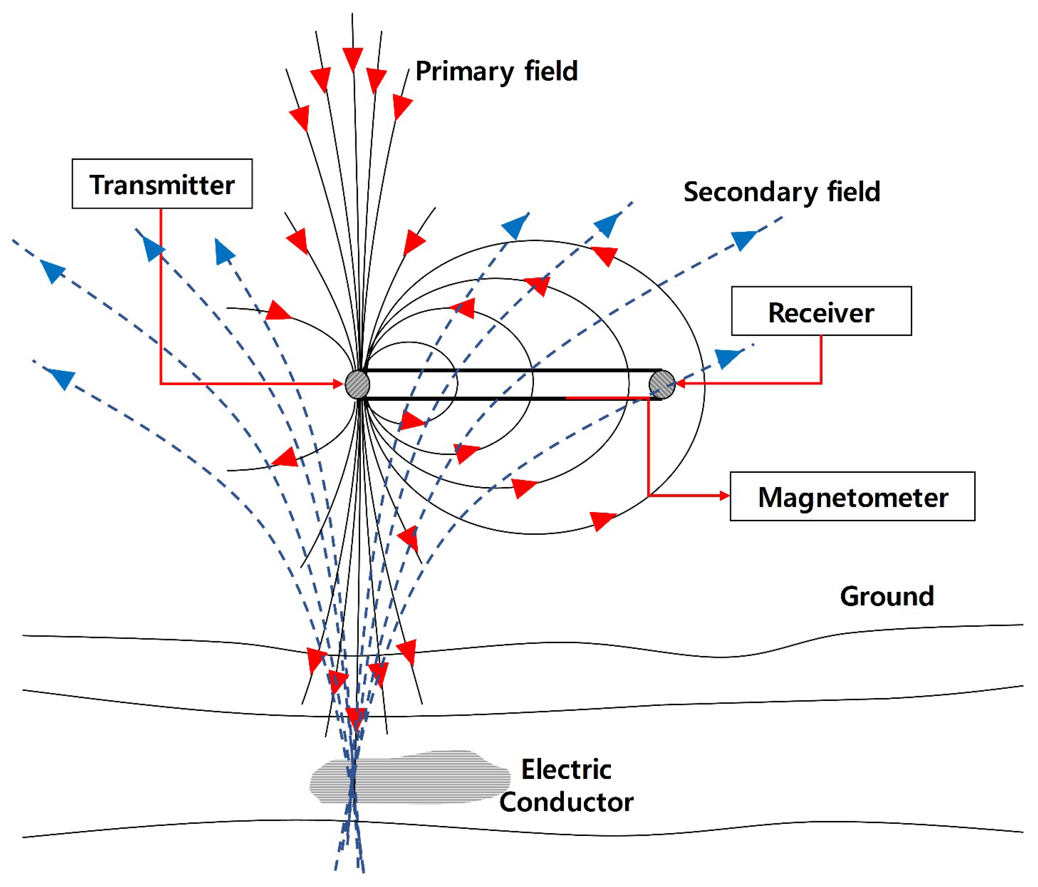
The basic principles of the FDEM exploration method are shown in Figure 1. The primary EM field develops around the transmission coils in accordance with Ampere’s law in the event that an alternating current with a range of frequency is transmitted to the coils. Then, a new current is induced in accordance with Faraday’s law when the primary EM field passes through an anomaly zone in the ground [13]. The new current induced in the anomaly zone forms a secondary EM field, which includes an in-phase component with the same phase as the primary EM field and a quadrature component with a 90° different phase from the primary EM field at the same time. The in-phase and quadrature components of the secondary EM field are divided by the primary EM field to obtain the transmittance of the EM field and, consequently, calculate the EC. The EC can be easily converted to ER because they have a reciprocal relationship.

2.2. Penetration Depth of the Electromagnetic Wave

EM waves can penetrate isotropic nonconductive objects to infinity without decreasing [4]. If the object is a good conductor, however, the penetration depth of the EM wave will decrease. Therefore, EM exploration techniques are extremely useful in cases where the surveyed object is a good conductor [14]. The penetration depth of an EM wave can be calculated using Equation (1) [13].

$$\delta =\sqrt{\frac{2}{w\mu \sigma }}\approx 500\sqrt{\frac{\rho }{f}}$$

(1)

where

• δ = penetration depth (m);
• w = circular frequency (rad/sec);
• μ = permeability (Hz/m);
• σ = EC (S/m);
• ρ = ER (ohm⸱m);
• f = used frequency (Hz).

The penetration depth, $\delta$, increases as the used frequency, f, which is set by the equipment, decreases. This is expressed by Equation (1) for the case where the ER of the object is constant. It implies that the properties of an object located deep underground can be obtained using a low frequency and vice versa when using a higher frequency. Therefore, equipment with an appropriate frequency range for the depth to be surveyed should be employed. In addition, the penetration depth, $\delta$, can be varied by decreasing the EM wave according to the permeability, $\mu$. The penetration depth, $\delta$, can also be varied according to the circular frequency, $w$, which can be used in inverse operations after noise elimination.

The penetration depth is also affected by the geometric composition of the equipment’s transmitter and receiver. When using FDEM exploration equipment, surveys can be performed for different depths by varying the composition of the number and spacing of the transmitter and receiver [11]. For instance, the CMD Mini Explorer used in this study is capable of surveying three different depths to a maximum depth of 1.56 m by using one transmitter and three receivers spaced 0.32, 0.71, and 1.18 m from the transmitter [15].

It should be noted that the ER of the ground is low when a large amount of water is present [16]. Therefore, a lower ER should be expected at deeper survey depths where the water content is generally higher than at shallower depths.

3. Test Plan

3.1. Exploration Targets in the Testbed

In 2017, the Korea Expressway Corporation constructed a testbed with a width of 5–6.6 m and a total length of 120 m in its road safety facility to evaluate nondestructive exploration techniques for road pavement subsurfaces. Various types and sizes of objects were embedded under asphalt pavement, concrete pavement, and an approaching slab in the testbed. Subsurface exploration was performed on eight asphalt pavement sections. The sections were selected as asphalt pavement is the main urban pavement type. The asphalt pavement section was comprised of the following layers: 50 mm of surface asphalt, 70 mm of intermediate asphalt, 150 mm of an asphalt base, 200 mm of an aggregate subbase, and 130 mm of an anti-freezing aggregate [17].

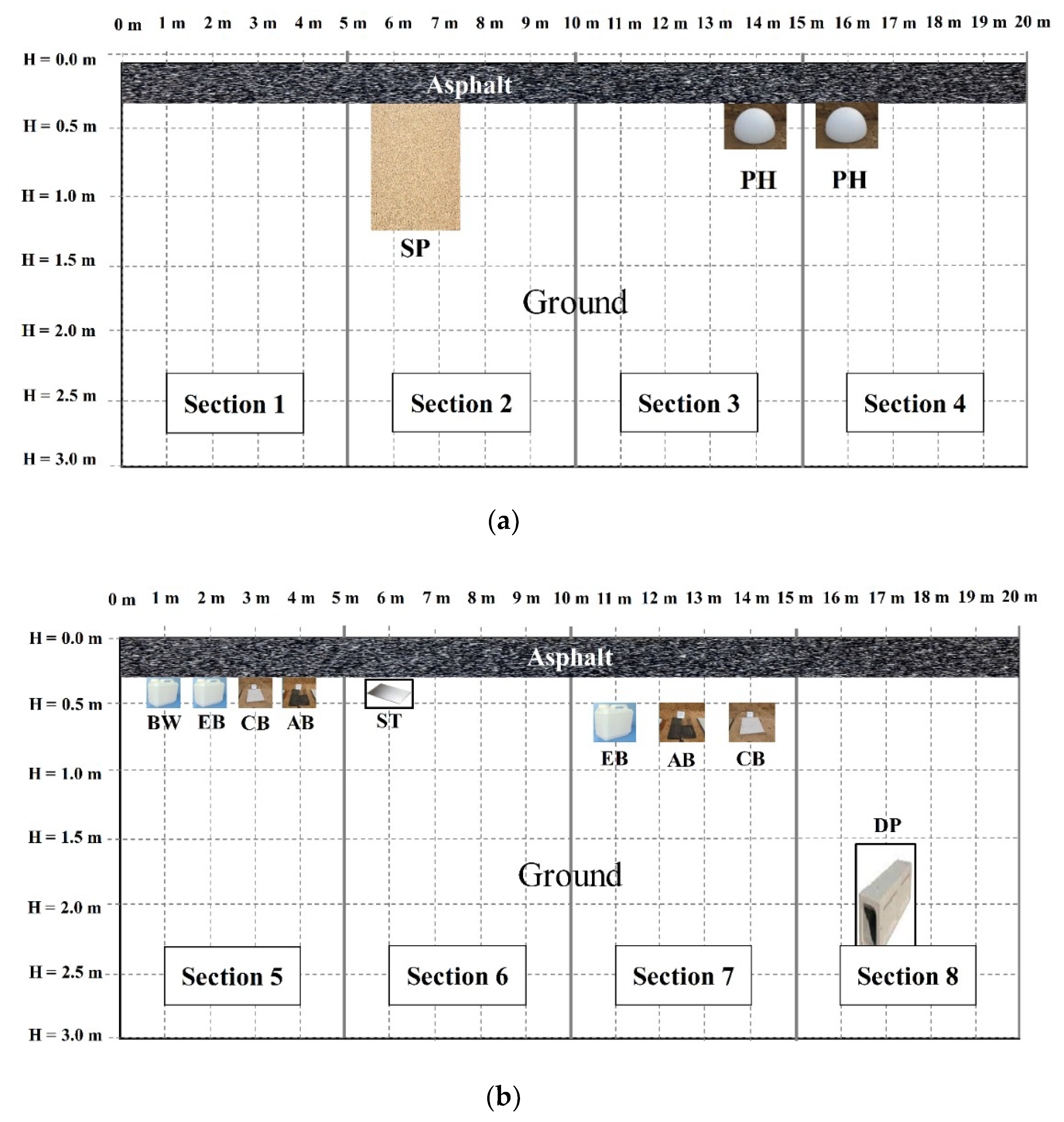
The objects embedded in each testbed section are listed in

Table 1. Facilities installed in the ground of the testbed.

Section No.	Facility	Abbreviation	Size (m)	Shape	Depth (m)
1	Natural Ground	-	-		-
2	Sand and Polystyrene Particles	SP	2 $\times$ 1.8 $\times 0.5$	Cuboid	0.55
3	Polystyrene Hemisphere	PH	R 0.5	Hemisphere	0.45
4	Polystyrene Hemisphere	PH	R 0.5	Hemisphere	0.45
5	Bottle Filled with Water	BW	0.5$\times$0.5$\times$0.1	Cuboid	0.35
	Empty Bottle	EB	0.5$\times$0.5$\times$0.1	Cuboid	0.35
	Concrete Block	CB	0.5$\times$0.5$\times$0.1	Cuboid	0.35
	Asphalt Block	AB	0.5$\times$0.5$\times$0.1	Cuboid	0.35
6	Steel Plate	ST	0.5$\times$0.5$\times$0.1	Cuboid	0.55
7	Empty Bottle	EB	1$\times$1$\times$0.1	Cuboid	0.55
	Concrete Block	CB	1$\times$1$\times$0.1	Cuboid	0.55
	Asphalt Block		1$\times$1$\times$0.1	Cuboid	0.55
8	Drainage Pipe		3$\times$0.9$\times$0.9	Cuboid	1.95

. Cavities, areas of ground softening, and underground facilities were selected as the target objects as they represent the main causes of sinkholes. The ground where the target objects were placed was compacted until the degree of compaction returned to the original state. The use of polystyrene to simulate cavities in the ground was deemed appropriate as its dielectric constant is similar to that of air [18]. An empty plastic bottle was also used to simulate a cavity as it has similar insulation characteristics to air. Asphalt and concrete blocks were used to represent objects in the ground with insulation characteristics. In addition, surveys were performed on conductive objects, such as a bottle filled with water, metal, and reinforced concrete drainage pipe.

Figure 2 shows the side views of the eight target sections, each of which was 5 m in length. The natural ground under the asphalt pavement of Section 1 did not have any cavities, areas of softening, or underground facilities. Objects of various sizes and materials were used to simulate the cavities, areas of softening, and underground facilities and were installed at various depths in Sections 2–8.

3.2. Exploration Method

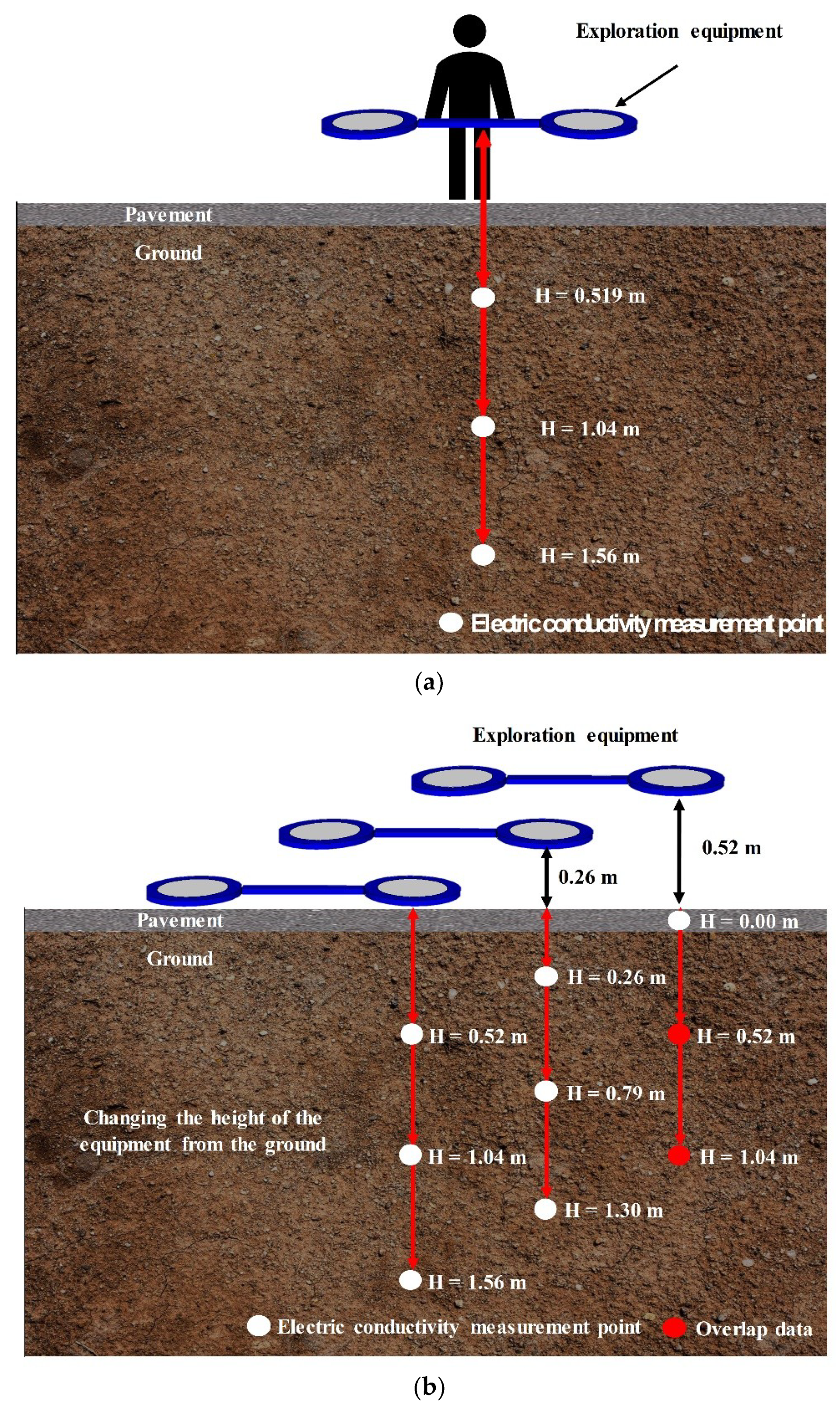
The CMD Mini Explorer used herein was able to survey depths of 0.52, 1.04, and 1.56 m using the equipment shown in Figure 3a. As a result, a tiny object was not able to be detected when it was situated between those distances. To overcome this weakness, the equipment was positioned at three different heights, including at the pavement surface, 0.26 m above the pavement surface, and 0.52 m above the pavement surface, to obtain data at depths of 0, 0.26, 0.52, 0.78, 1.04, 1.32, and 1.56 m below the pavement surface as shown in Figure 3b.

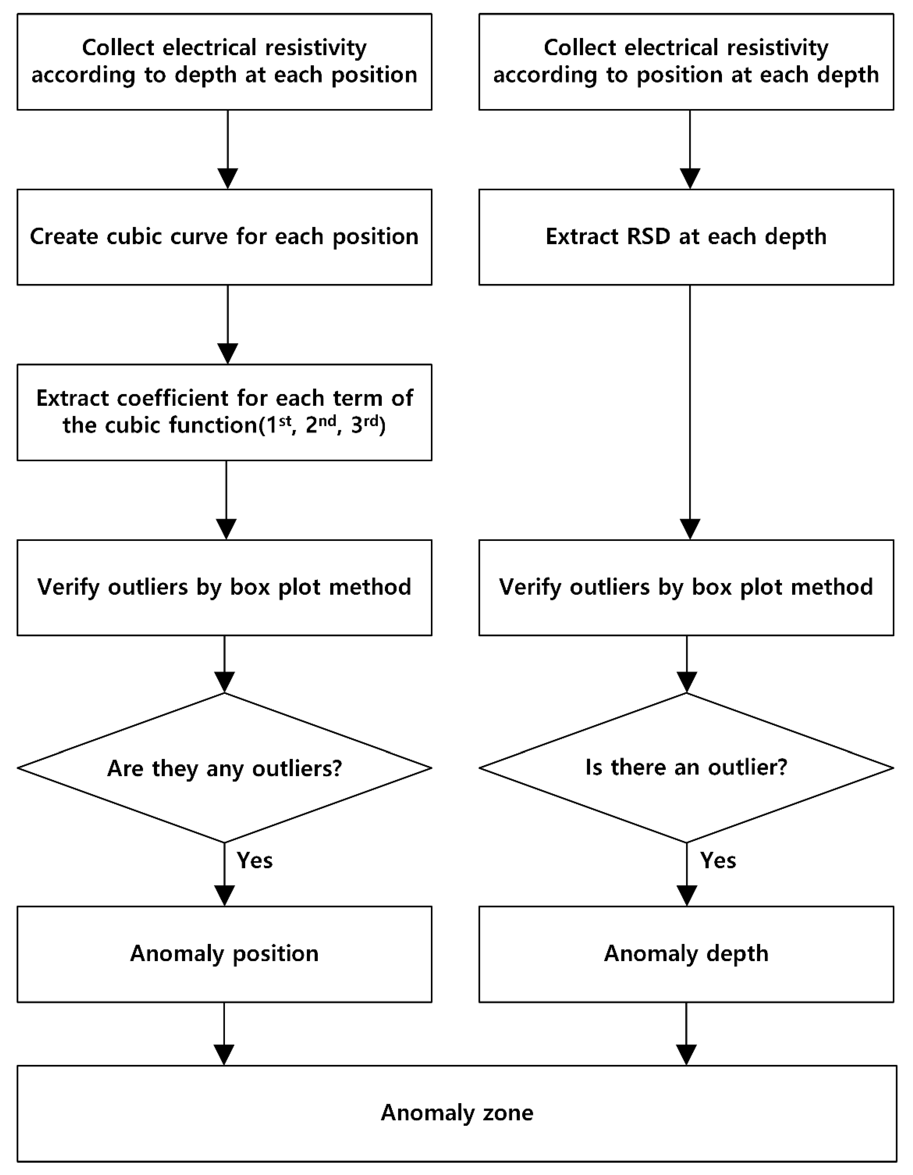
The EM properties of the subsurface were measured at 11 positions at 0.5m spacing in each section which is 5 m in length. It took about 5 s to measure each position. The equipment was set to a frequency range of 18 kHz to measure the three different depths concurrently. The EC was calculated by measuring the in-phase component and quadrature component of the secondary EM field. The calculated EC was stored and plotted by the equipment. Then, the ER was calculated by obtaining the reciprocal of the EC. The quantitatively expressed ER was then converted to a two-dimensional (2D) ER contour map using the inverse operation program of the CMD Data Transfer developed by GF Instruments Company to evaluate the distribution of the ER and detect the anomaly zones via visual inspection. In addition, the calculated ER was analyzed via a statistical method following the procedure shown in Figure 4 to detect the anomaly zones quantitatively.

4. Detection of Anomaly Zones by Visual Observation

4.1. Natural Ground

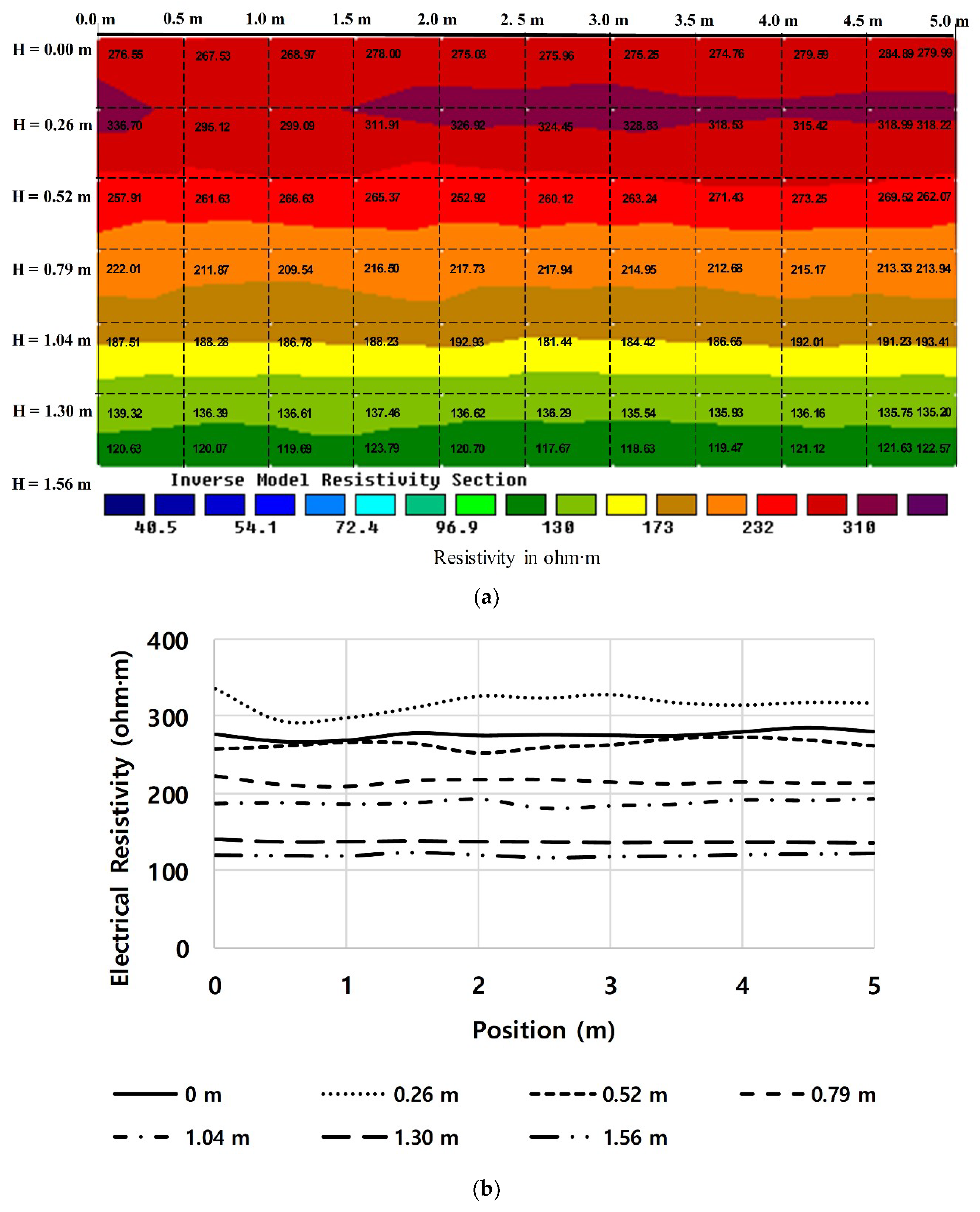
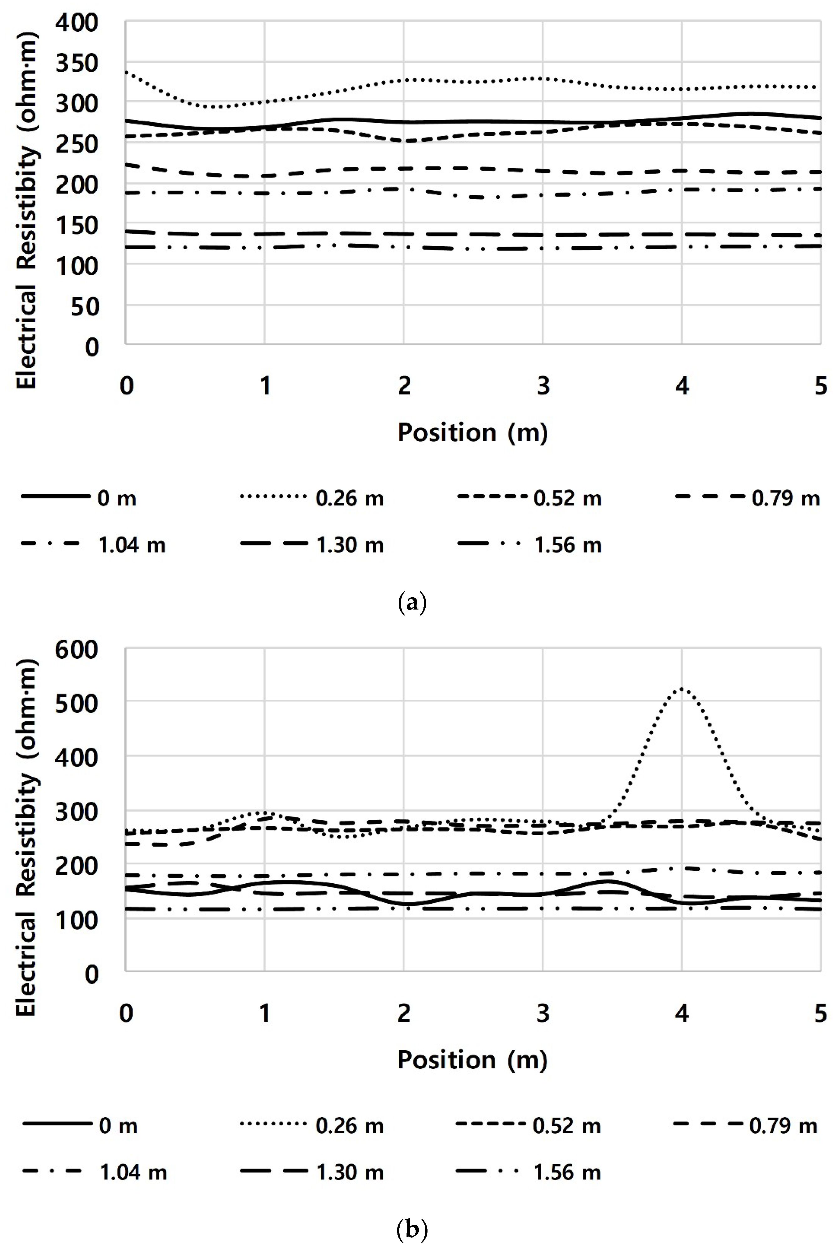
Figure 5a shows a 2D ER contour map of the natural ground in Section 1. No anomaly zones were detected by visual observation because the ER exhibited a nearly uniform distribution across the map with no significant variations. In addition, the ER gradually lessened as the depth increased. Figure 5b shows the graph of the ER of the natural ground according to the measurement position for each depth. The graph shows that the ER was constant without any significant changes according to the measurement position for all depths. The ER was the largest at depths of 0 and 0.26 m by about 300 ohm⸱m and was smallest at a depth of 1.56 m by approximately 120 ohm⸱m. It was estimated that the decrease in the ER according to the depth was mainly caused by the fact that the natural ground was not a perfect isotropic nonconductor. Hence, the EM wave decreased the farther down it penetrated. In addition, it was estimated that the lower ER in the deeper parts of the ground was affected by the increased amount of water at those depths.

4.2. Areas of Cavities

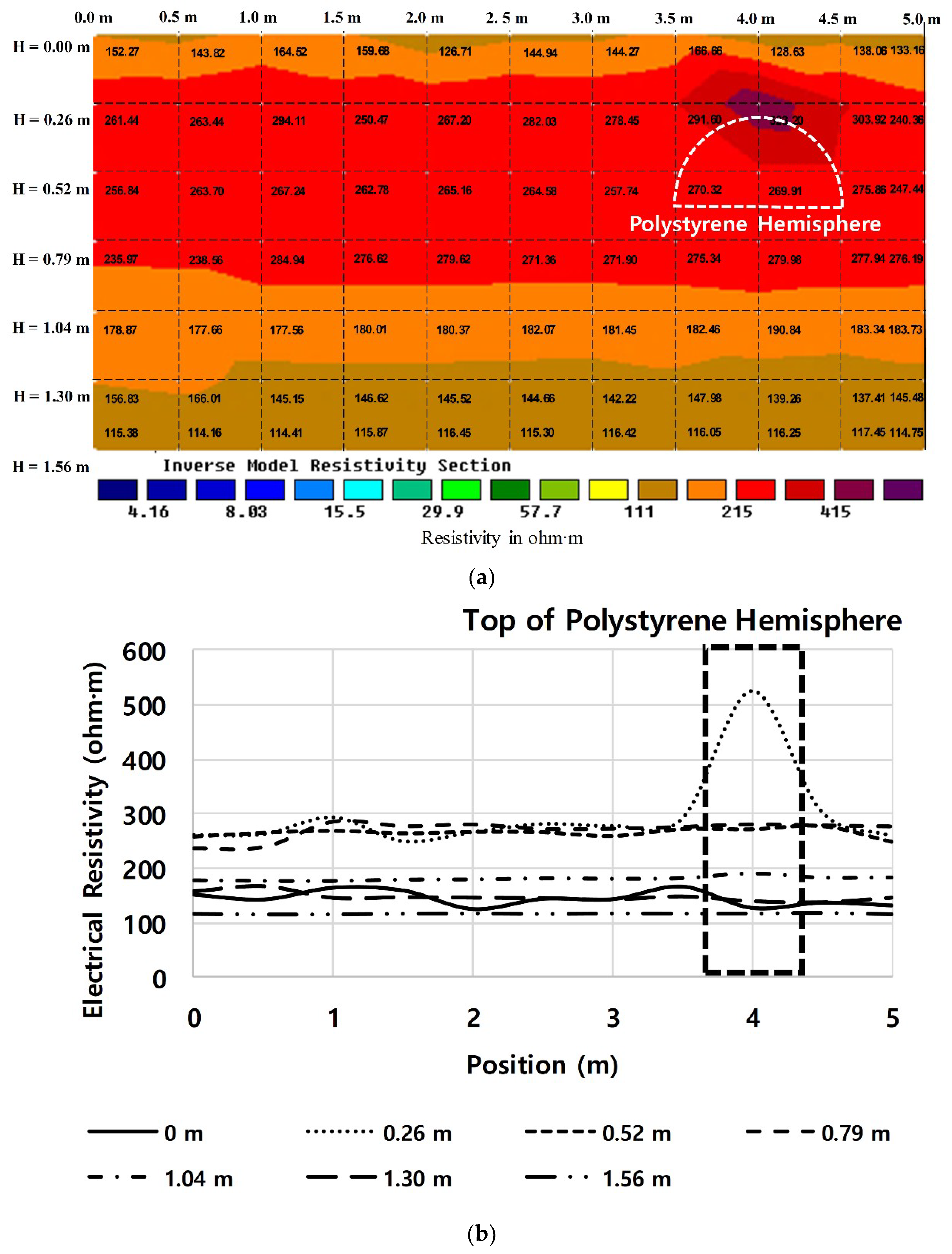
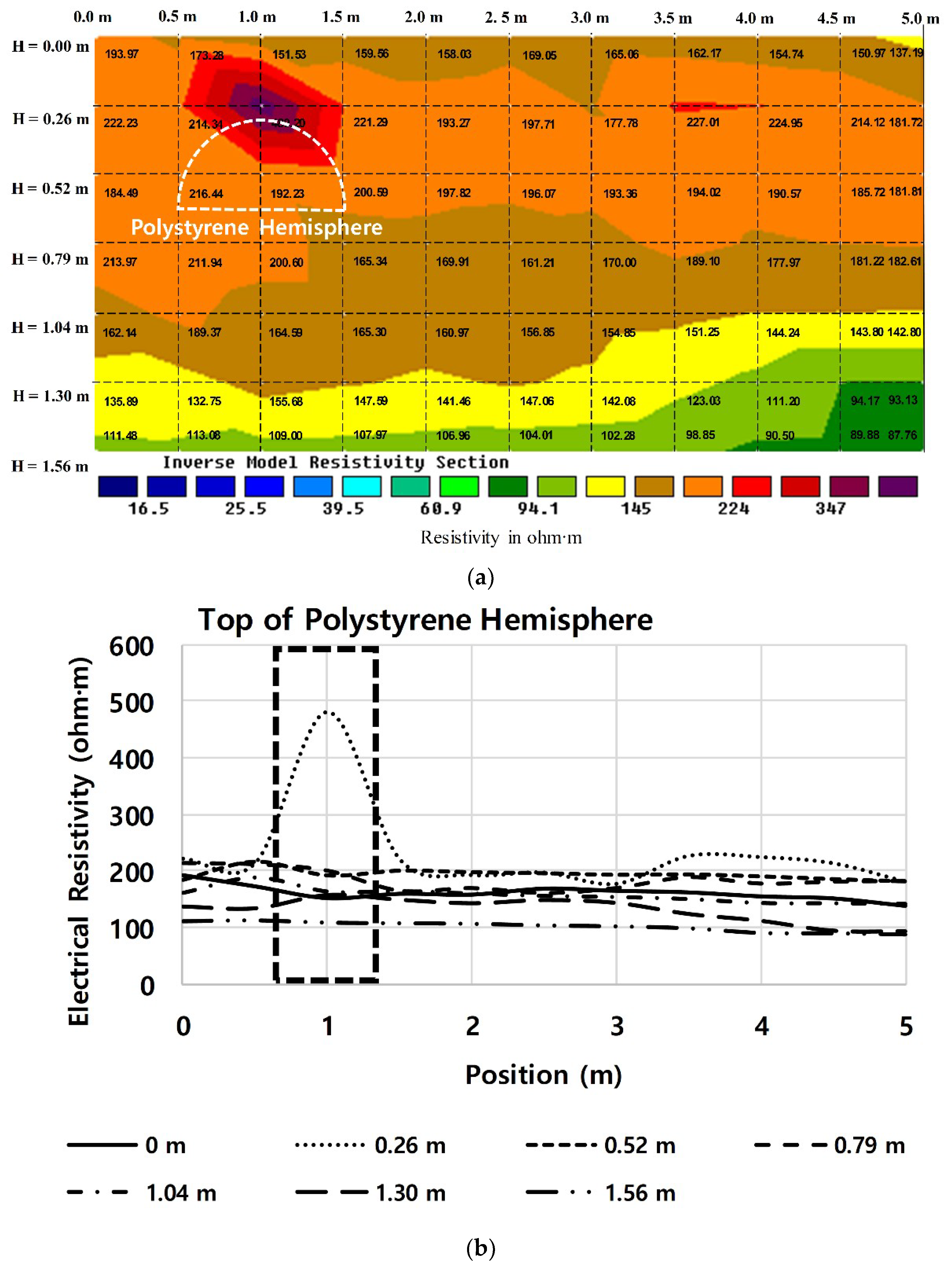
Figure 6a and Figure 7a show the 2D ER contour maps of Sections 3 and 4, where the polystyrene hemispheres were installed at 4 and 1 m, respectively, with each buried at a depth of 0.45 m. As shown in the maps, the anomaly zones that exhibited a significantly large ER revealed the locations of the polystyrene hemispheres and could be detected on the contour maps by visual observation. Figure 6b and Figure 7b show the graphs of the ER in each section measured according to the depth of each position. The tops of the cavities were also identified via the increase in the ER at 4 and 1 m and at a depth of 0.26 m for Sections 3 and 4, where the tops of the polystyrene hemispheres were located.

Yu and Carin [19] reported that the receiving rate of the transmitted EM wave could decrease in cases where the scale of the nonconductive object was large in the direction of the wave propagation. Therefore, it was estimated that the receiving rate of the transmitted EM wave would decrease when it penetrated the 0.5 m radius of the polystyrene hemispheres, as they were relatively large compared to the capacity of the equipment used in this study. It was also estimated that the higher ER that appeared only at the top of the object was caused by the current channeled at top of the polystyrene hemisphere. Thus, the ER in the lower part of the polystyrene hemispheres was lower than at the top of the polystyrene hemispheres and appeared to be similar to that of the surrounding ground.

4.3. Areas of Ground Softening

Figure 8a shows the 2D ER contour map for Section 2, which included an area of ground softening simulated by a mix of sands and polystyrene particles. The pocket of softened ground, which was 2 (L) × 1.8 (W) × 0.5 m (T), was located at position 1.5 m at a depth of 0.55 m. The ER in the area was significantly larger than that of the surrounding natural ground. The higher ER of the softened ground was distributed over its actual size, as shown in Figure 8b, where the ER is presented on the graph according to the measurement position by depth. The higher ER of the softened ground was attributed to the fact that water could easily percolate through the sands and polystyrene particles, resulting in a much lower water content than the surrounding natural ground. Consequently, the ER of the softened ground was higher than that of the surrounding natural ground over its actual area, whereas the ER of the cavities simulated by the polystyrene hemispheres was larger only at the top of the cavities.

4.4. Underground Facilities

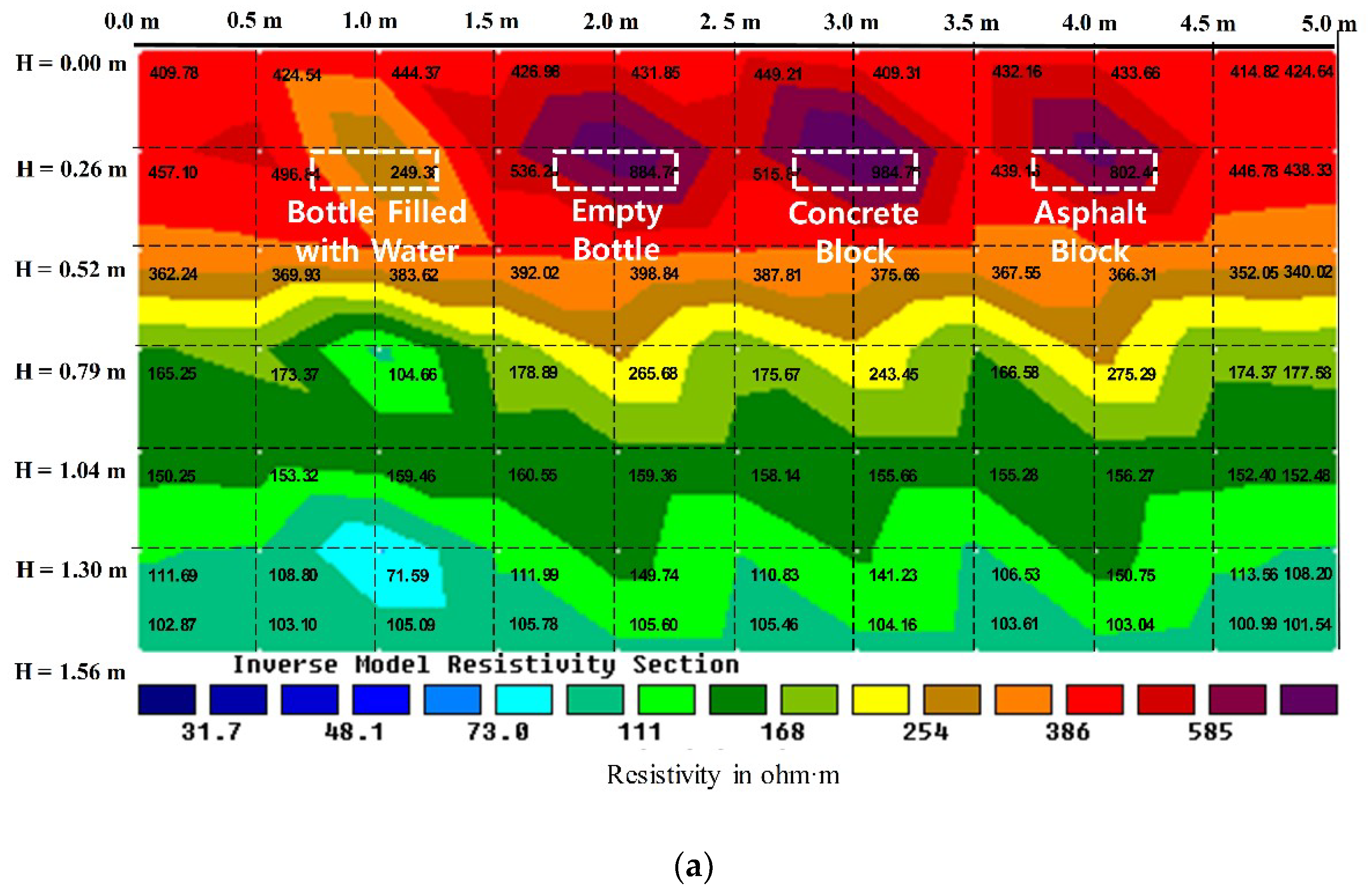
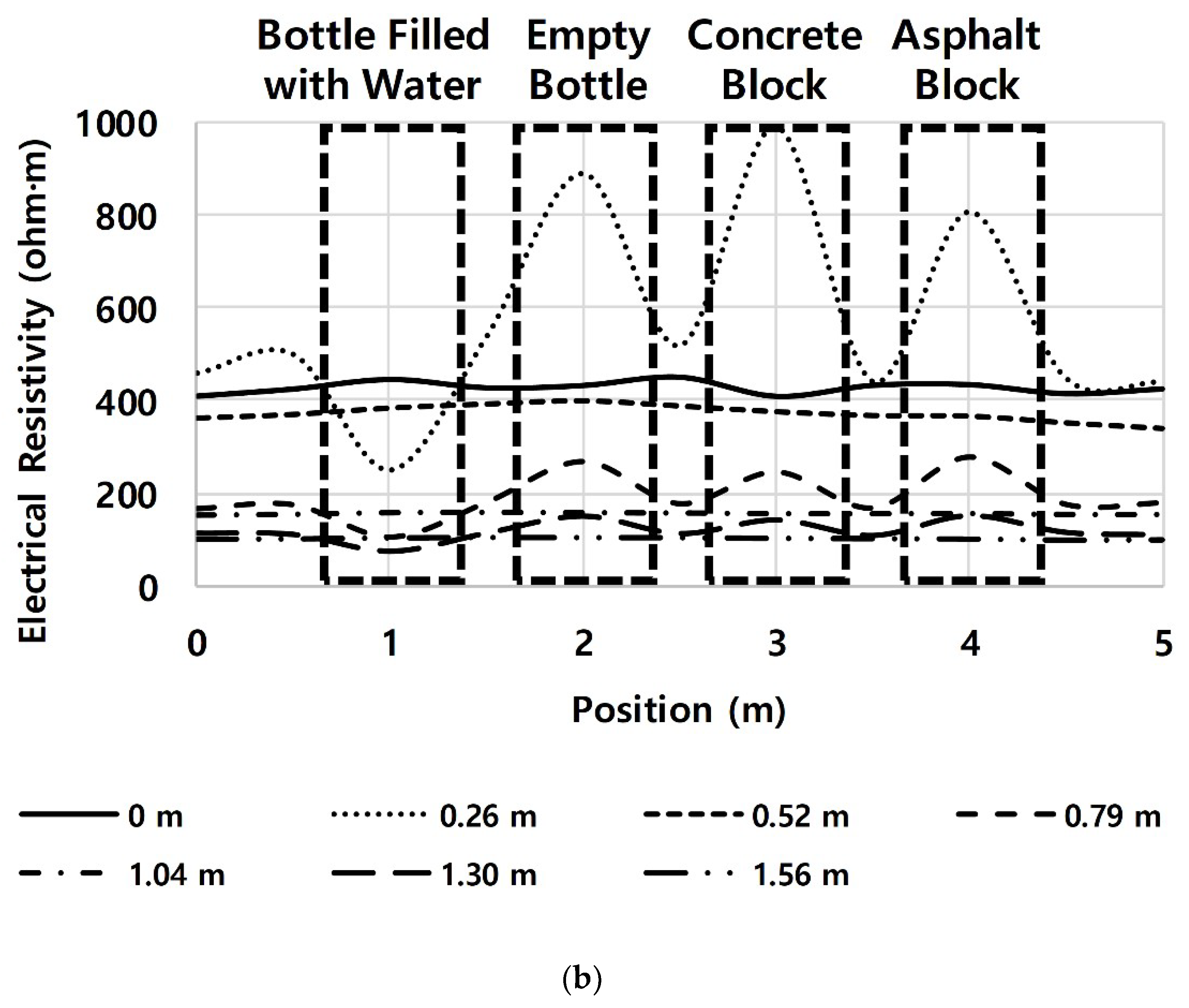
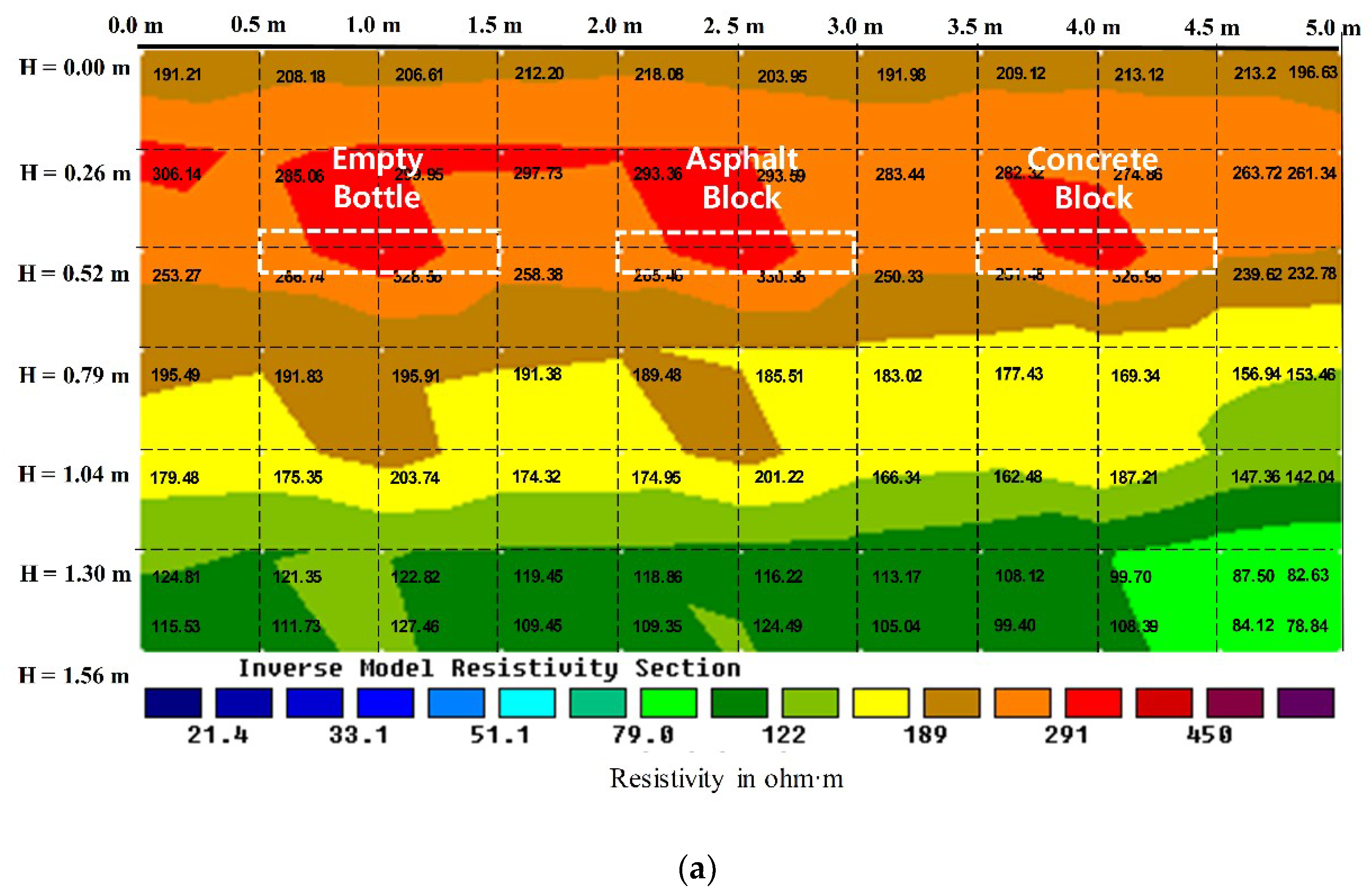
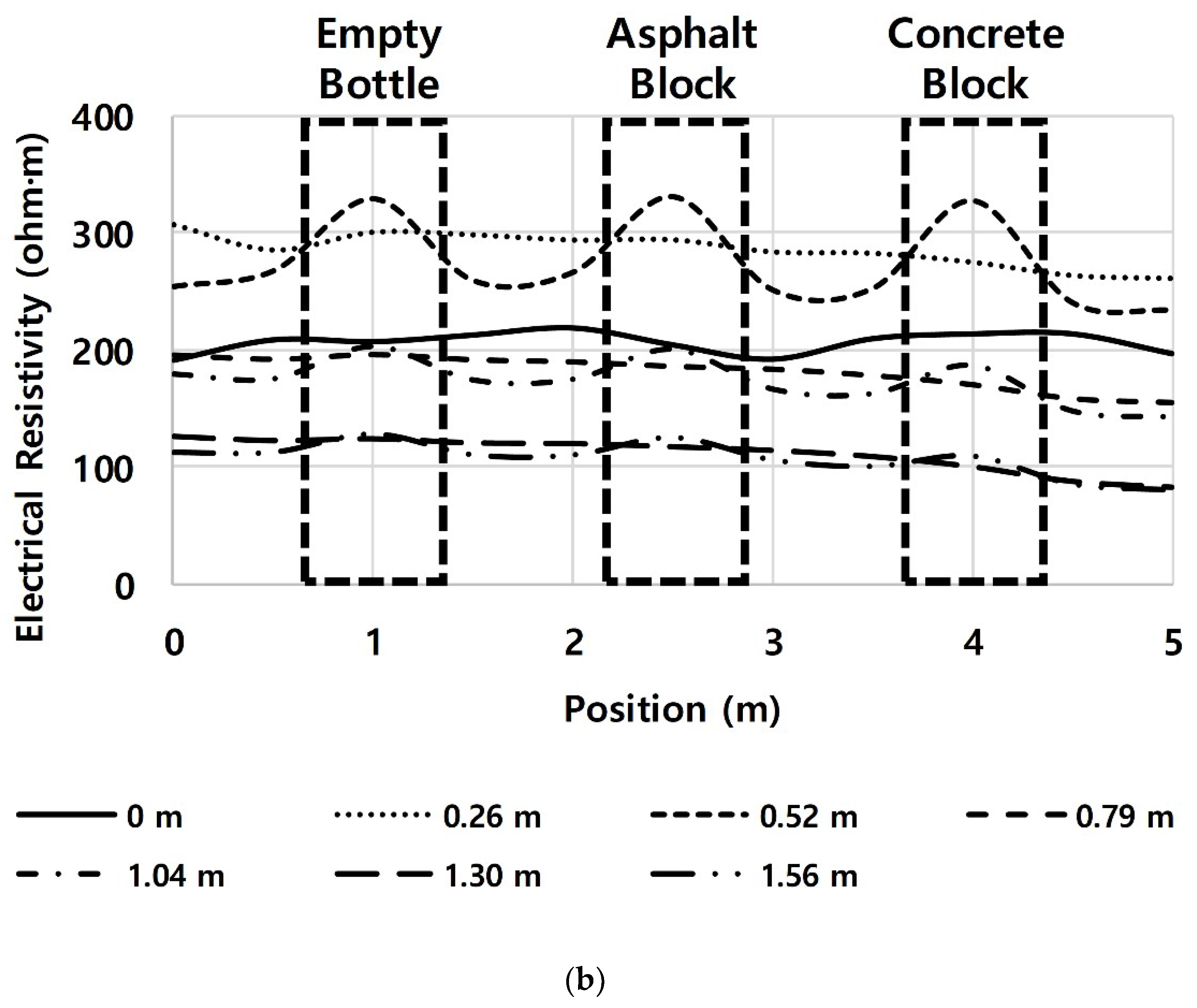
Figure 9a shows the 2D ER contour map of the ER distribution in Section 5. This section is where the bottle filled with water, empty bottle, concrete block, and asphalt block (0.5 × 0.5 × 0.1 m in size) were each installed at a depth of 0.35 m. They were laid at 1, 2, 3, and 4 m, respectively. Figure 10a shows the 2D ER contour map of Section 7 in Figure 2, where an empty bottle, asphalt block, and concrete block (1 × 1 × 0.1 m in size) were each installed at a depth of 0.55 m. They were installed at 1, 2.5, and 4 m, respectively. The empty bottle represented a cavity in the ground, while the asphalt and concrete blocks represented rocks or other artificial structures that might exist in the ground. Each item had nonconductive characteristics, while the bottle filled with water had conductive characteristics.

As shown in Figure 9a and Figure 10a, the empty bottle, asphalt block, and concrete block, which had nonconductive characteristics, exhibited higher ER than the surrounding ground, whereas the bottle filled with water exhibited lower ER. The ER was nearly constant at each measurement position for all depths except 0.26 m, which was where the underground facilities were installed, as shown in Figure 9b. At a depth of 0.26 m, the ER significantly varied at the measurement positions where the facilities were installed. The ER significantly decreased at the measurement position where the bottle filled with water was located, owing to its conductive characteristics, whereas the ER increased at the measurement position of the empty bottle, concrete block, and asphalt block because they were nonconductive. Similarly, the ER was nearly constant for all depths at measurement positions where no facilities were installed, whereas the ER significantly varied according to the measurement position at a depth of 0.52 m, where the underground facilities were installed, as shown in Figure 10b.

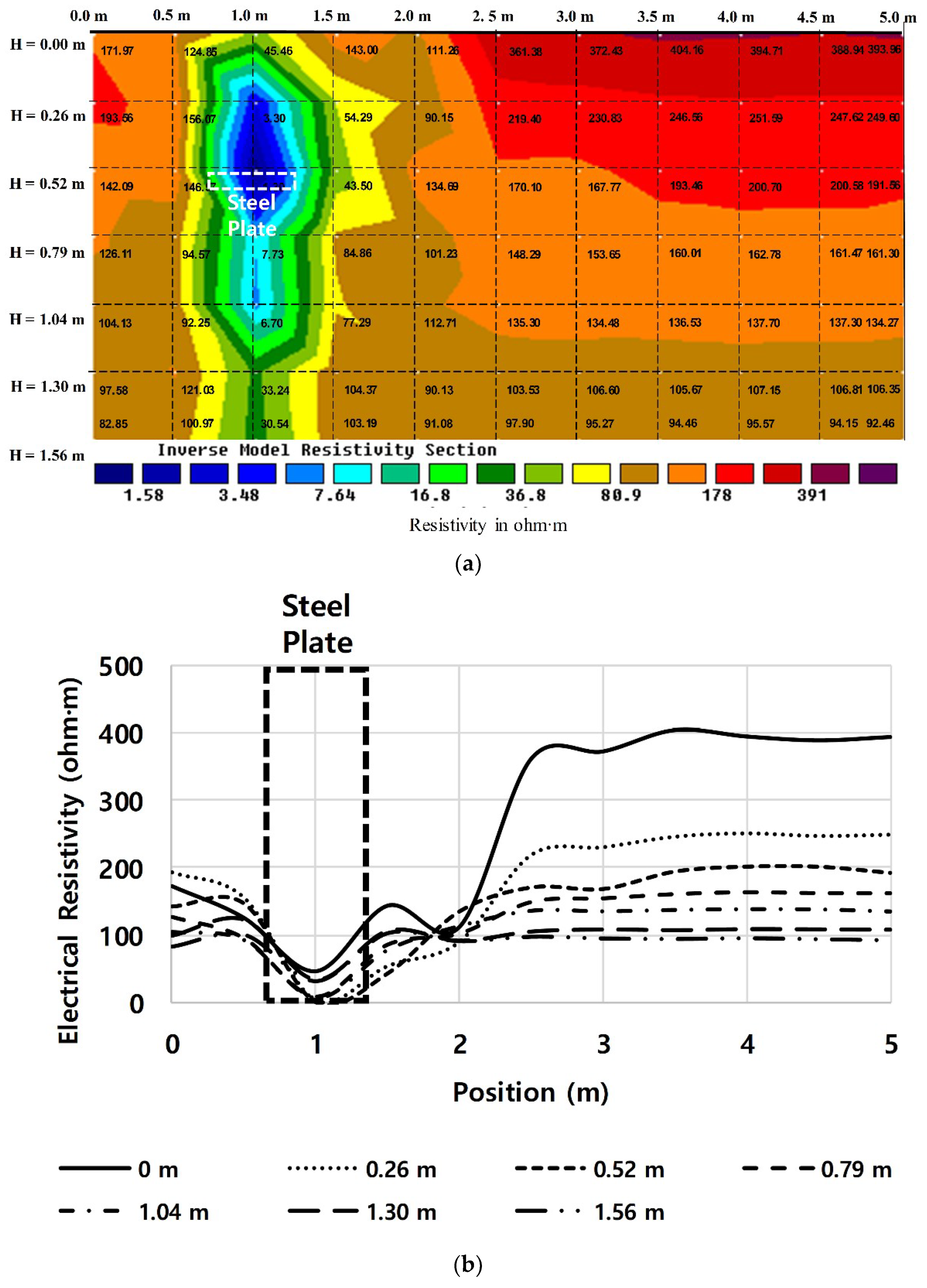
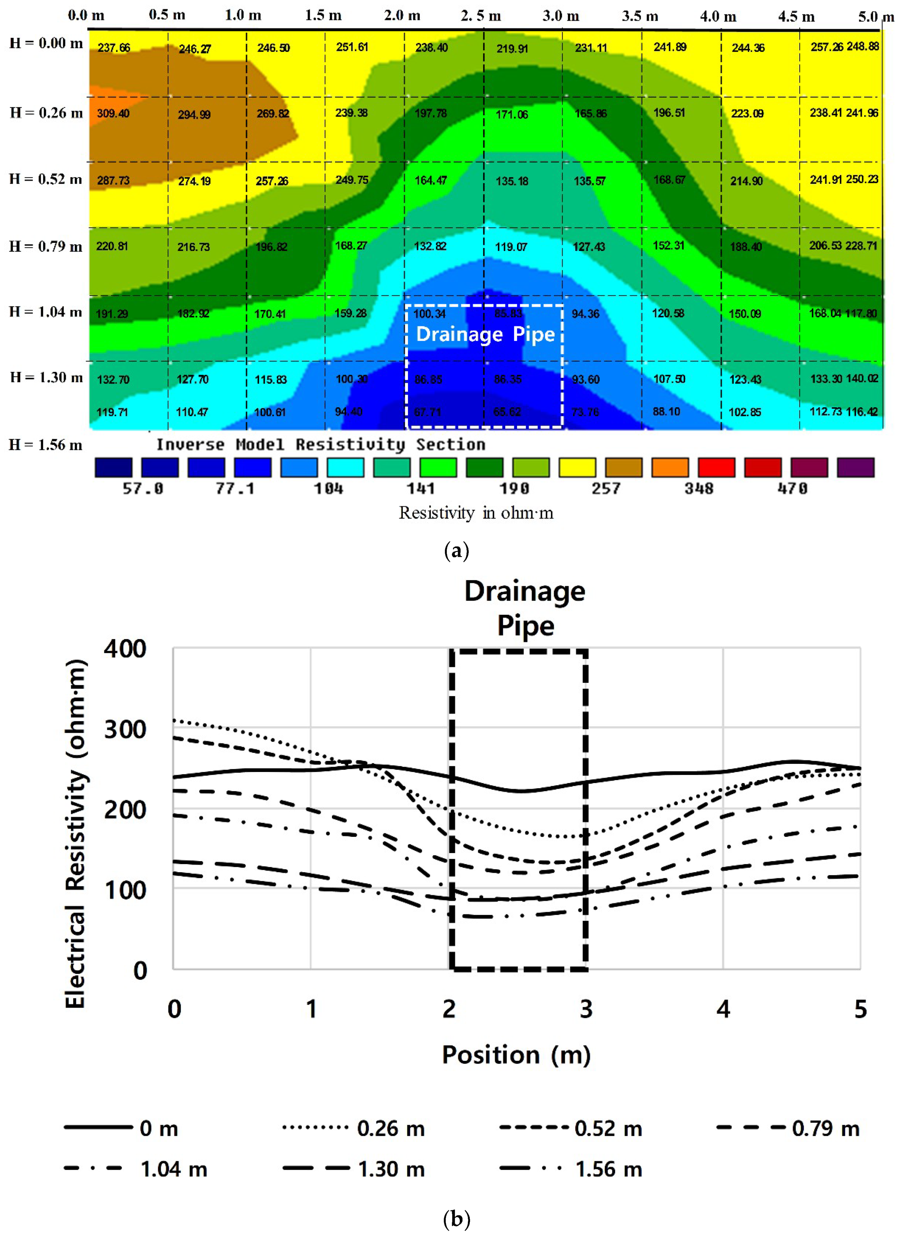
Figure 11a and Figure 12a show the 2D ER contour maps of Sections 6 and 8 where the steel plate and drainage pipe were installed, respectively. The steel plate was 0.5 × 0.5 × 0.1 m in size and was laid at 1 m at a depth of 0.27 m, while the drainage pipe was 3 × 0.9 × 0.9 m in size and was laid at 2.5 m at a depth of 1.95 m. The steel plate was used to represent a conductive material, whereas the drainage pipe was a reinforced concrete structure comprised of both conductive and nonconductive materials. The ER of the steel plate was lower than that of the surrounding ground and was distributed over a much wider area than the actual size of the steel plate, as shown in Figure 11a. The lower ER of the steel plate and its corresponding distribution over a wider area than its actual size is also shown in Figure 11b. The ER of the reinforced concrete drainage pipe was also lower than that of the surrounding ground and was distributed over a much larger area than the actual size of the drainage pipe, as shown in Figure 12a. The lower ER of the drainage pipe and its corresponding distribution over a larger area than its actual size is shown in Figure 12b. As a result, it was determined that an accurate identification of the location and size of conductive metallic underground facilities with this method was difficult, whereas the mere existence of such facilities could be easily verified.

5. Detection of Anomaly Zones by Statistical Methods

5.1. Anomaly Position

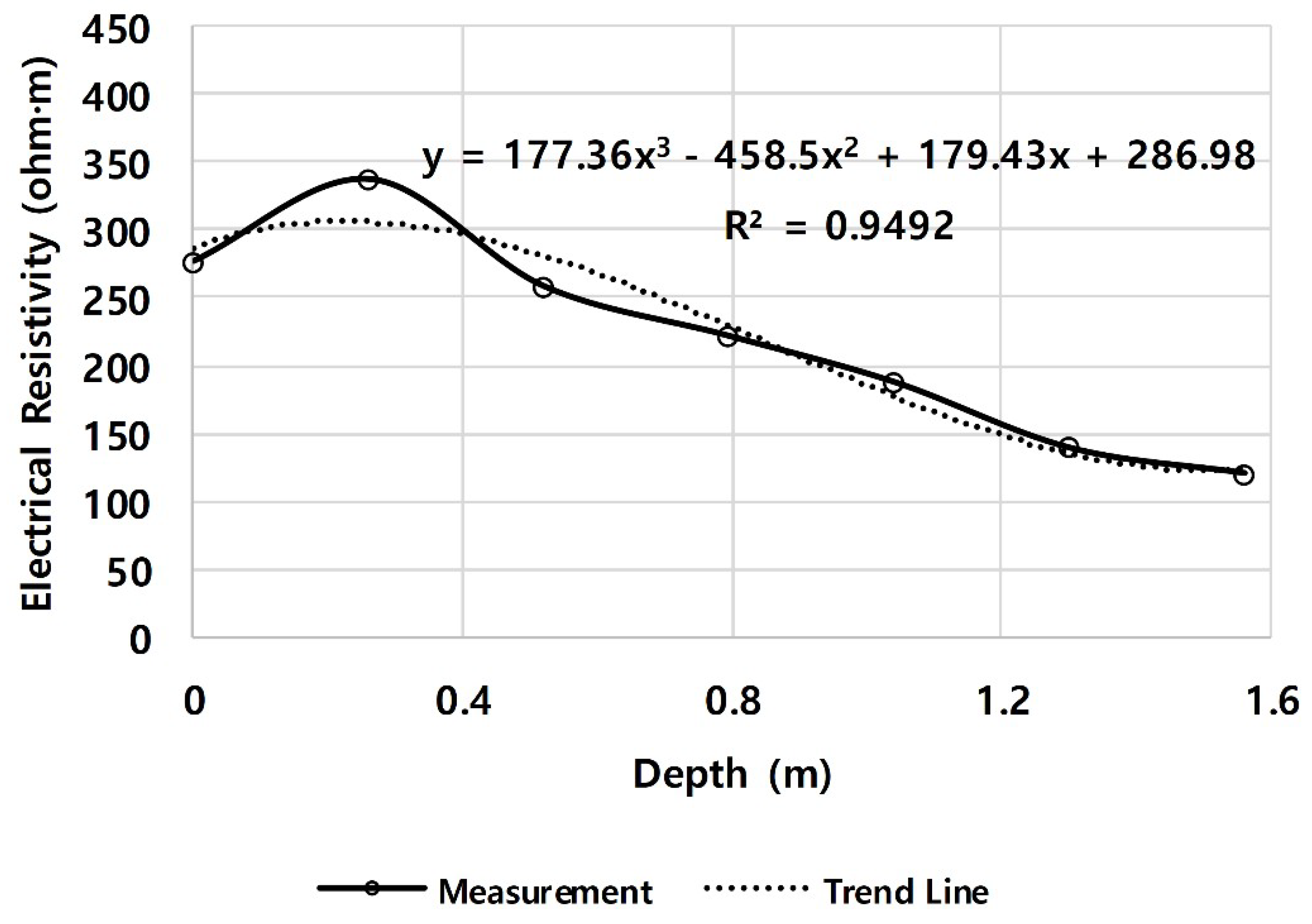
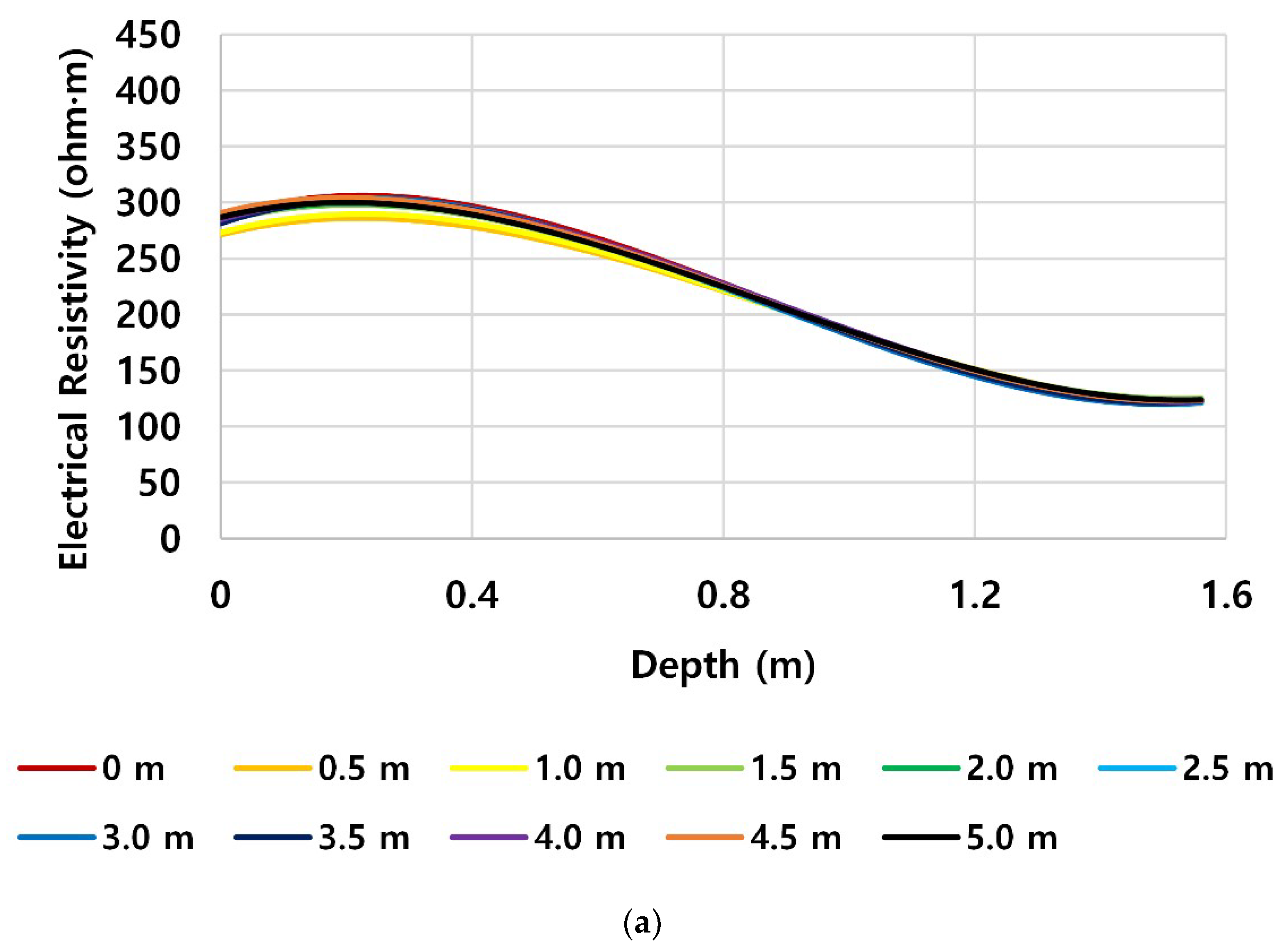
The natural ground in Section 1, where no anomaly zones were present, exhibited a higher ER at shallower depths and a lower ER at deeper depths, as shown in Figure 13. The distributions of the ER of the natural ground were well expressed by a cubic curve according to the depth and were similar at all measurement positions, as shown in Figure 14a. 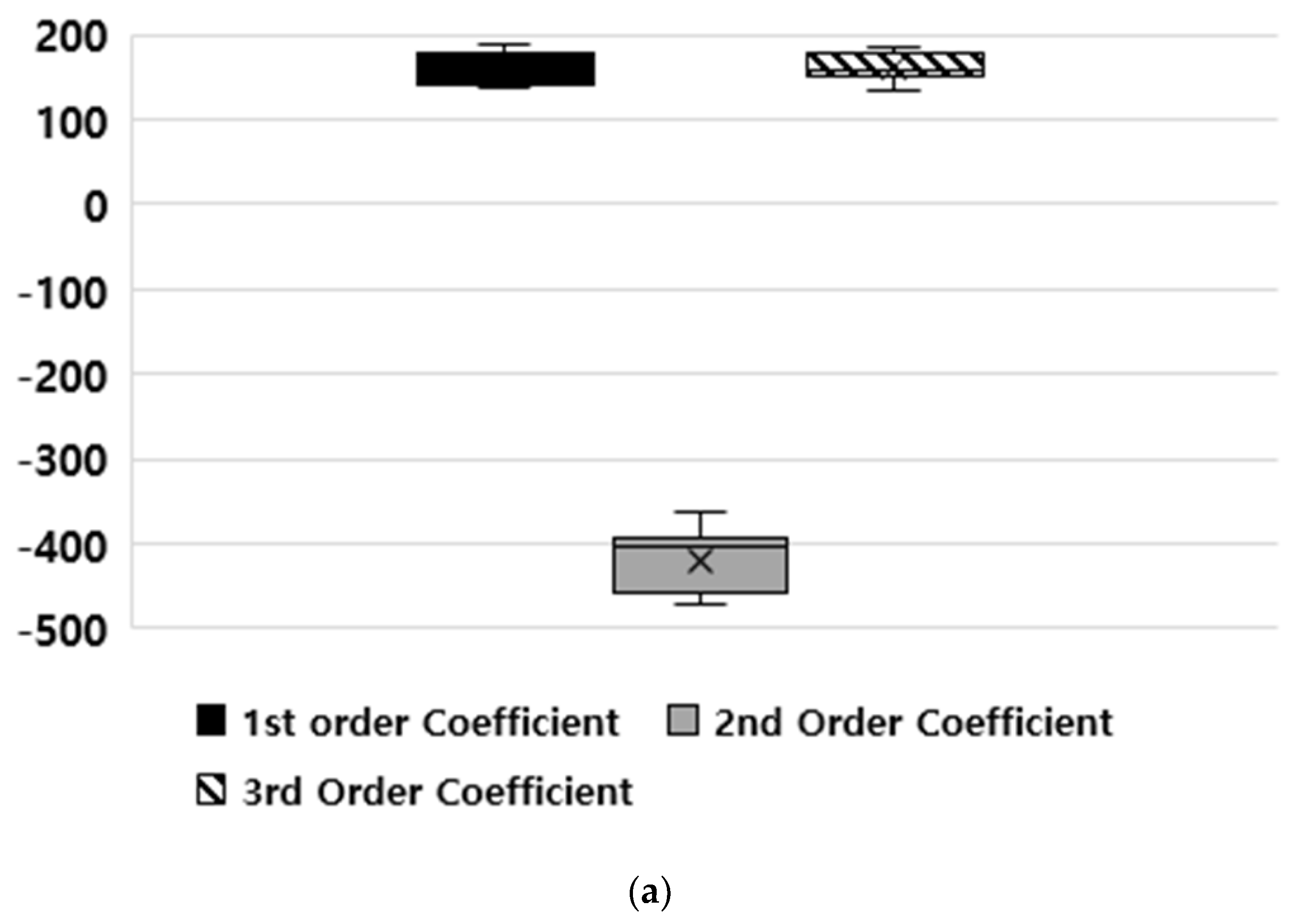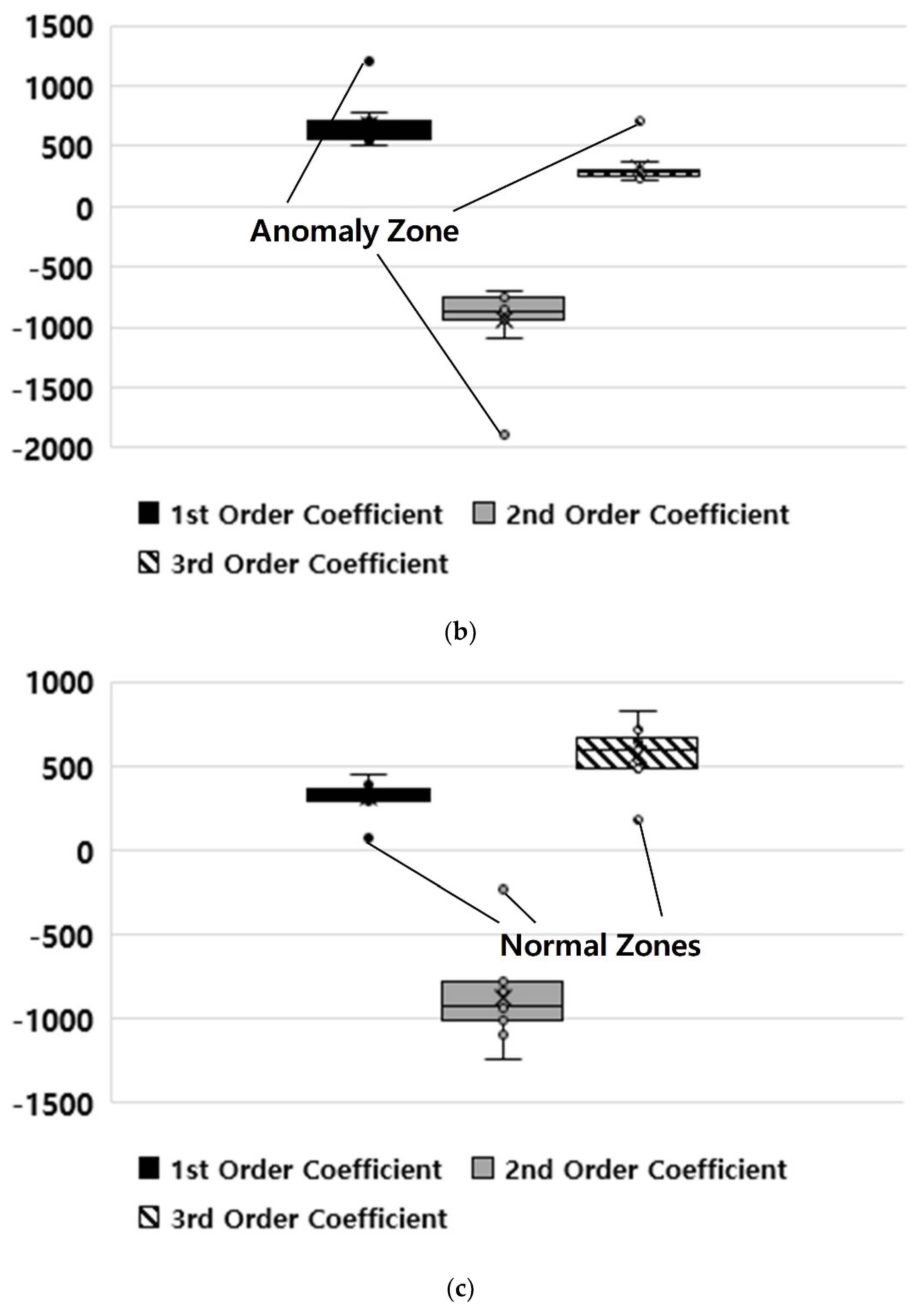However, the trend of the cubic curve at the position where the polystyrene hemispheres were installed in Section 3 was different from that of other positions, as shown in Figure 14b. Therefore, the coefficients of each term (i.e., the first, second, and third terms) of the cubic function obtained at each measurement position were distributed in box plots by section to identify any outliers, as shown in Figure 15. The difference between the first and the third quartile was defined as the interquartile range (IQR). The values smaller than the first quartile minus the IQR and the values larger than the third quartile plus the IQR were defined as outliers.

No outliers were identified for the natural ground in Section 1 as no anomaly zones existed there. This can be observed in Figure 15a as the trend of the ER according to the depth was similar at all measurement positions. In Section 3, where cavities were simulated using polystyrene hemispheres, an outlier was identified from each term of the cubic function at the position where the top of the polystyrene hemisphere was located, as shown in Figure 15b. Anomaly zones were simulated at several locations in Sections 5 and 7, while a single large anomaly zone was simulated in Section 2. In these cases, the measurement positions of the anomaly zones occupied 4/11 to 9/11 of the total measurement positions. As a result, the positions where anomaly zones did not exist were plotted on the box plots as outliers, as shown in Figure 15c. Therefore, during actual exploration work for which a large anomaly zone or several anomaly zones are expected, a sufficient length for the individual measurement sections should be determined.

5.2. Anomaly Depth

The ER of the natural ground in Section 1, where no anomaly zones existed, increased with the depth and exhibited a relatively constant value according to position for all depths, as shown in Figure 16a. The ER also increased with depth and was nearly constant according to position in Section 3, whereas the ER significantly changed at the location of the anomaly zone, as shown in Figure 16b. As a result, the positions of the anomaly zones can be found by comparing the trend of the cubic curves generated at each measurement position. However, the ER according to position cannot be expressed by a cubic curve because the ER was nearly constant for each measurement position at all depths. Therefore, the relative standard deviation (RSD) of the ER was used to identify the depth of the anomaly zone quantitatively.

The RSD is generally used to compare the relative magnitudes of the standard deviation of data sets with different means. The RSD is calculated by dividing the standard deviation by the arithmetic mean as shown in Equation (2).

$$RSD=\frac{\sigma }{\overline{x}}$$

(2)

where

• RSD = relative standard deviation;
• $\sigma$ = standard deviation;
• $\overline{x}$ = arithmetic mean.

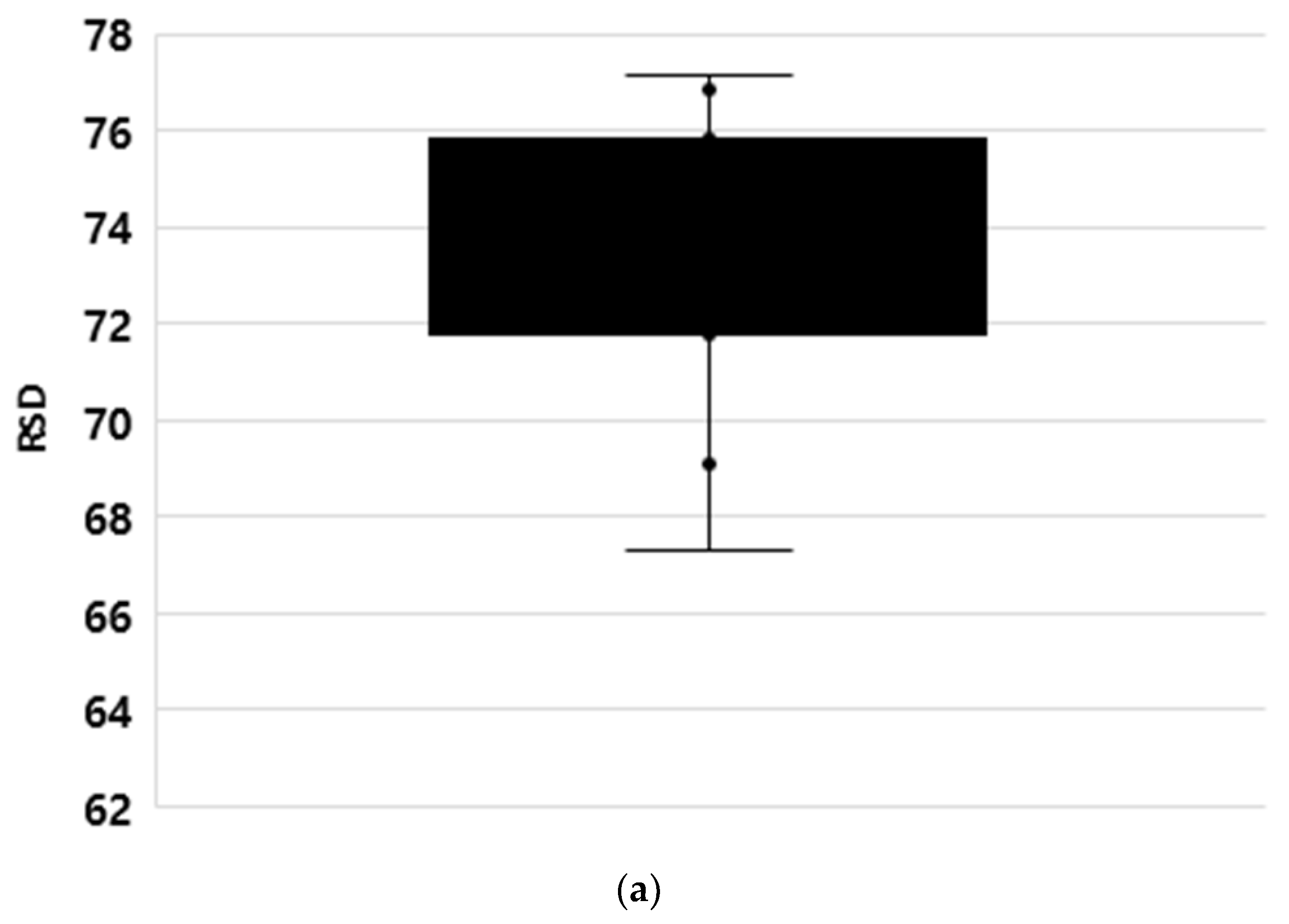
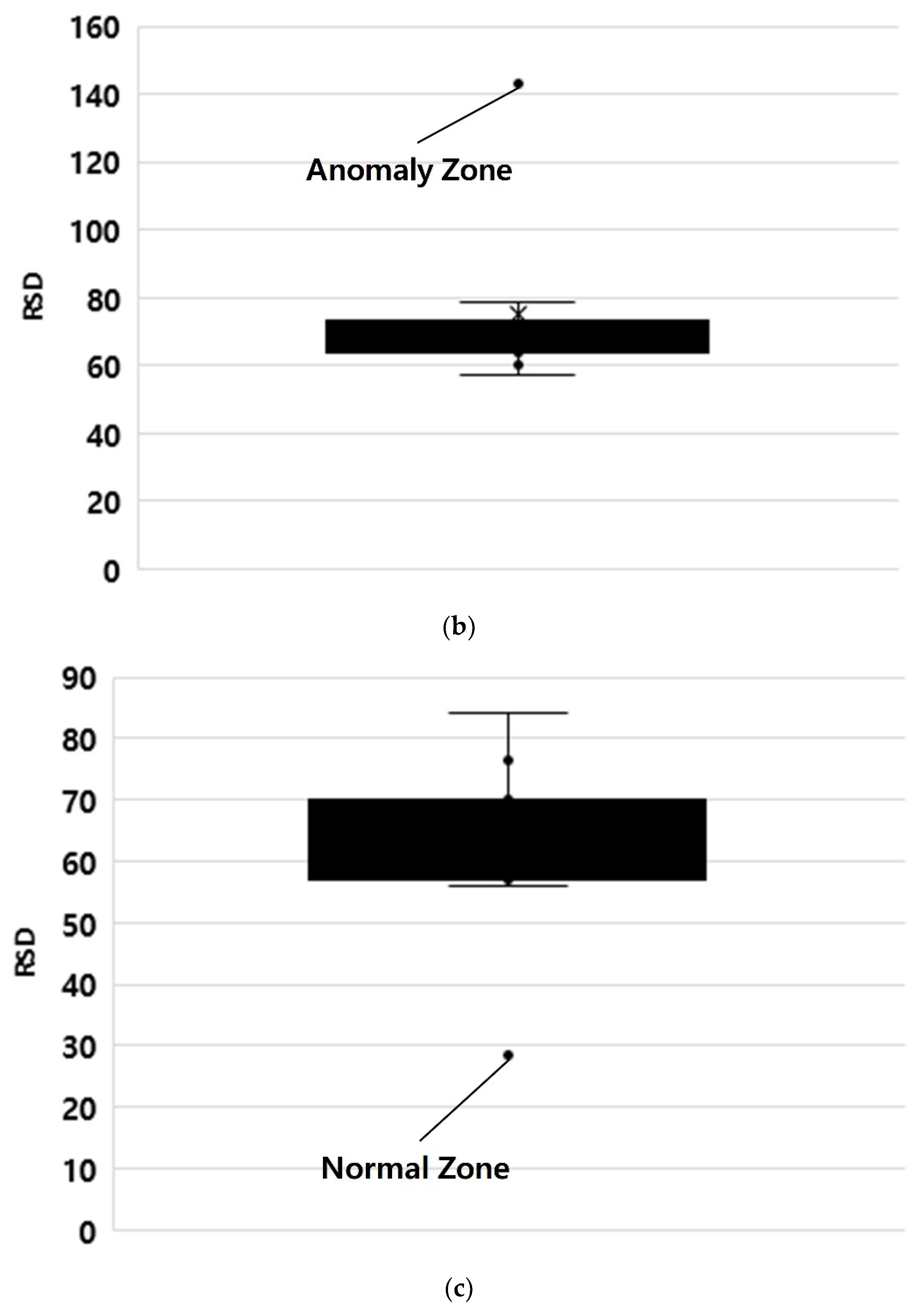
The outliers were found by distributing the RSDs calculated by the means and standard deviations of the ER according to position on a box plot by depth. In Section 1, where no anomaly zones existed, no outliers were identified on the box plot, as shown in Figure 17a. However, in Section 3, where an anomaly zone existed, the depth of the actual anomaly zone was identified as the outlier, as shown in Figure 17b.

In Section 2, where a single large anomaly zone was simulated, the measured depths of the anomaly zones occupied 3/7 of the total measured depths. In this case, the depth where an anomaly zone did not exist was plotted as an outlier, as shown in Figure 17c. In cases where several anomaly zones exist at various depths in the same position, even though this case was not prepared in the testbed, the depths at which an anomaly zone does not exist may also be presented as outliers on the box plot. Therefore, a sufficient number of measured depths should be determined to facilitate surveying of the locations where a large anomaly zone or several anomaly zones are expected.

6. Conclusions

In this study, cavities, areas of ground softening, and underground facilities were detected using the small-loop EM exploration method. The anomaly zones were qualitatively detected by visual observation using colored contour maps. In addition, a statistical method for detecting anomaly zones quantitatively was employed. The main conclusions of this study are as follows:

A method for taking survey measurements at several heights and superimposing the results was utilized to increase the number of measured depths to compensate for the capacity weakness of the EM exploration equipment. Thus, survey results with high resolution can be obtained for multiple depths using only one piece of equipment.

The ER gradually decreased as it penetrated farther down into the natural ground. This was attributed to the fact that the EM wave decreased as a result of changes in the water content with the depth.

The top of the cavities, which were simulated using polystyrene hemispheres, exhibited a much higher ER than that of the surrounding ground. However, the lower part of the polystyrene hemisphere showed a similar ER to that of the surrounding ground. It was estimated that the higher ER that appeared only at the top of the polystyrene hemisphere was caused by the current channeled at the location. Interestingly, the softened ground, which was simulated using a mix of sand and polystyrene particles, exhibited a higher ER than that of the surrounding ground over its entire area. It was estimated that the higher ER that appeared at the entire area of softened ground was also caused by the current channeled at the top of each sand and polystyrene particle.

The nonconductive facilities installed in the ground showed a significantly higher ER than the surrounding ground, whereas the conductive facilities exhibited a lower ER. The steel plate and reinforced concrete drainage pipe showed a significantly higher ER than the surrounding ground over a much larger area than their actual size. Hence, the locations of these facilities cannot be accurately detected. Their existence, however, could be easily verified.

A statistical method for detecting cavities, areas of ground softening, and underground facilities using a box plot and the RSD method was employed. The positions of the anomaly zones were identified by plotting the coefficients of each term of the cubic functions of the ER according to depth on a box plot and identifying the outliers. In addition, the depths of the anomaly zones were detected by plotting the RSDs of the ER according to the position calculated for each depth on a box plot and identifying the outliers.

It was determined that the portable EM exploration equipment used in this study can be applied to small-scale roads with narrow widths, park roads, sidewalks, etc., which are different from the applications of large-scale exploration equipment. In addition, it was determined that cavities, areas of ground softening, and underground facilities can be detected quantitatively using the statistical method, which was an improvement on the previous method that detected anomaly zones qualitatively by visual observation of the 2D ER contour map.