Article

Optimization of Grinding Parameters for the Workpiece Surface and Material Removal Rate in the Belt Grinding Process for Polishing and Deburring of 45 Steel

1
School of Aerospace Engineering, Xiamen University, Xiamen 361005, China
2
Zhejiang Provincial Engineering Lab of Laser and Optoelectronic Intelligent Manufacturing, Wenzhou University, Wenzhou 325024, China
*
Author to whom correspondence should be addressed.
Appl. Sci. 2020, 10(18), 6314; https://doi.org/10.3390/app10186314
Submission received: 29 December 2019 / Revised: 5 September 2020 / Accepted: 7 September 2020 / Published: 10 September 2020
(This article belongs to the Section Mechanical Engineering)

Abstract

:

Featured Application

Robotic polishing application; material surface polishing and deburring.

Abstract

Surface roughness and the material removal rate (MRR) are two important indicators during the grinding process. The former determines the surface quality while the latter reflects the grinding efficiency directly. In this paper, the two indicators are taken into consideration simultaneously and differently by converting them into a comprehensive goal with using weighting objective method. A prediction model was established for each comprehensive goal with each different combination of surface roughness and MRR weighting coefficient. The optimal value of abrasive size, contact force, belt linear speed, and feed speed were obtained under different grinding situations by using a central composite design (CCD) combined with response surface analysis. The experimental results showed that the comprehensive goal can be used effectively as an indicator to control the grinding performance and improve the optimization process.

1. Introduction

We commonly use 45 steel in the manufacture of various critical structural parts for its good mechanical properties and cheap price. For instance, 45 steel is a common material in the area of shaft-related parts manufacturing. The shaft parts must have high surface quality when coordinating with the bearings. In terms of bearing, the surface roughness of bearing raceway also has a significant influence on bearing noise [1]. Abrasive belt grinding is an effective way for polishing and deburring of 45 steel to achieve a smooth surface. However, in the actual mass production process, we want to improve material removal rate (MRR) to enhance production efficiency with good surface quality assurance at the same time, thereby saving costs and winning customers.
Grinding is the final processing procedure and an important step in determining product quality, and therefore merits special attention and study. Investigators have conducted a lot of studies on the optimization of process parameters in the field of grinding. Some research focused on increasing MRR on the basis of the prediction model of MRR. For example, Song et al. [2,3] built an effective material removal prediction model considering the influence of the curvature radius on the bonnet polishing. Liu et al. [4] established a machining mathematical model of MRR and optimized the processing parameters (cutting area, feed rate, and cutting speed) to achieve higher MRR in rotary ultrasonic grinding machining. Wu et al. [5] introduced a simulation platform that has the ability to predict MRR and achieve an optimal selection of the grinding process key parameters. Ho et al. [6] studied the process parameters and optimized the polishing parameters to enhance the MRR.
Some research strongly focused on reducing surface roughness determining optimal process parameters by establishing a surface roughness prediction model in order to get better product quality. Zhao et al. [7] and Yong et al. [8] investigated the grinding and grinding process of IBR of aero-engine and nHAP, respectively, while both established the surface roughness prediction model and optimized grinding parameters by using response surface methodology (RSM). Periyasamy et al. [9] found the optimum parameters for minimum surface roughness by using RSM with design expert software in the grinding process of AISI 1080 steel plates. In references [10,11,12,13], the Taguchi design method was widely used to optimize milling parameters for surface roughness. In fact, focusing on only a single goal will not meet the grinding requirements of an actual production process, since at least two objectives must be considered simultaneously.
In recent years, more research has focused on the multi-objective optimization of. Gopal et al. [14] developed a genetic algorithm (GA) code to optimize the grinding conditions for maximum material removal with using a multi-objective function model, by imposing surface roughness and surface damage constraints. Ting et al. [15] carried out the optimization of operating parameters to obtain optimum parameters via Particle Swarm Optimization (PSO) based on the objective of maximizing MRR with reference to surface finish and damage for silicon carbide grinding. Kumar et al. [16] studied the optimization of input parameters for maximizing the MRR and achieving optimum surface roughness with the help of Minitab software. Pai et al. [17] investigated three grinding variables for simultaneous optimization of MRR and surface roughness with using RSM and enhanced elitist non-dominated sorting genetic algorithm (enhanced NSGA-II), respectively, and proved that the enhanced NSGA-II is effective. Kumar et al. [18] developed empirical models for surface roughness and MRR by considering grinding parameters (wheel speed, table speed, and depth of cut) as control factors using RSM and obtained the optimum machining parameters which can lead to minimum surface roughness and maximum MRR. Sedighi et al. [19] presented an approach using an integrated Genetic Algorithm-Neural Network (GA-NN) system to optimize the creep feed grinding (CFG) process, aimed to obtain the maximal MRR and the minimum of the surface roughness. Lee et al. [20] used compressed air to minimize specific grinding forces and surface roughness while maximizing specific material removal rate (MRR), conducted a multi-objective optimization and got the optimal values of depth of cut, feed rate and air temperature towards minimum surface roughness and maximum specific MRR. However, most of the research described above focused on optimizing MRR and surface roughness regarding one as a constraint or considering both as independent goals. Only a few studies have attempted to convert the two objectives of surface roughness and MRR to an integrated one to do the optimization.
The purpose of this article is to find out the optimal grinding parameters for the 45 steel. The critical parameters that affect the surface roughness and polishing efficiency such as abrasive size, contact force, belt linear speed, and feed speed, were examined. RSM with CCD was used to select polishing conditions (abrasive size, contact force, belt linear speed, and feed speed) in order to obtain the minimal surface roughness and maximal grinding efficiency. This research of 45 steel grinding would be useful in the grinding and grinding industries. Meanwhile, the multivariable optimization method is widely used in scientific research. The research method in this paper has significant reference value for other researchers.
This paper is organized as follows: Section 2 introduces the design of the mechanical system of a grinding machine; Section 3 presents a single factor experiment and the application of CCD; Section 4 describes an optimization example and obtains the optimum grinding parameters; Section 5 shows a simple laboratory experiment to validate the effect of this method and Section 6 proposes some concluding remarks and prospects.

2. Mechanical System Design

According to the technical requirements of robot belt grinding, the robot belt grinding system is designed (see Figure 1). Robot is the center of this grinding system, it can catch the workpiece from the feeding station, and then complete the scheduled grinding track relying on its own programming. After the completion of grinding, the workpiece will be returned back to the feeding station. The series of actions of the robot can finally help to achieve automatic grinding.
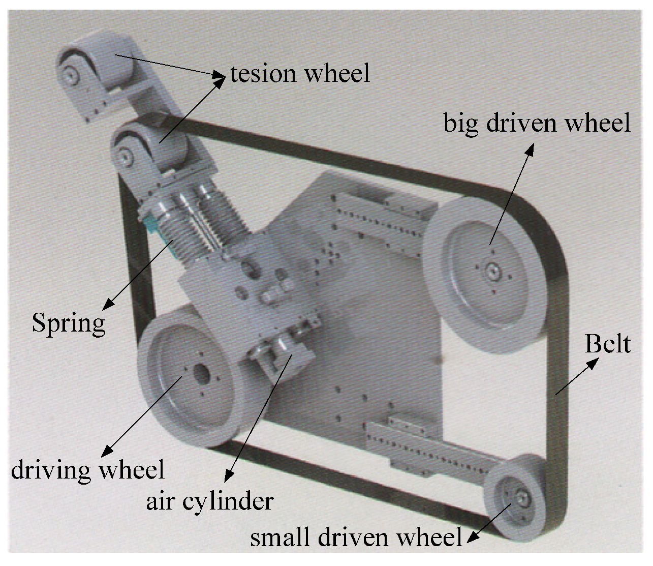
In order to maintain constant belt tension force during the grinding process, the pneumatic tensioning mechanism is designed to fulfill the pressure requirement. A belt transmission and tensioning system are established, as we can see in Figure 2. The belt tension force can be changed by controlling the regulating valve of a floating pneumatic cylinder.
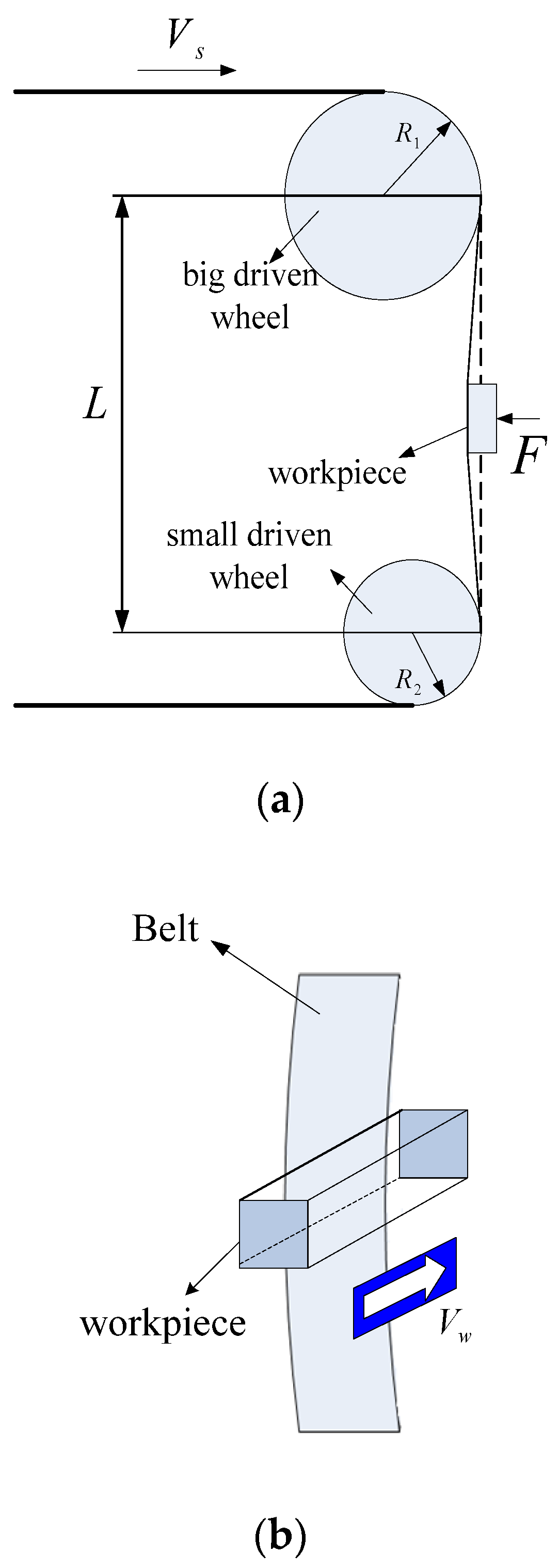
Figure 3 shows the schematic depiction of the abrasive belt grinding, in the case of abrasive grinding, important parameters that affect abrasion are abrasive size, contact force, belt linear speed, and feed speed. Different experimental conditions may lead to different results, so it is absolutely essential to note the working conditions and workpiece characteristics before belt grinding. The chemical composition of 45 steel, main characteristics of the workpiece, and grinding condition are shown in Table 1, Table 2 and Table 3, respectively.

3. Experiment Procedure

3.1. Experiment Preparation

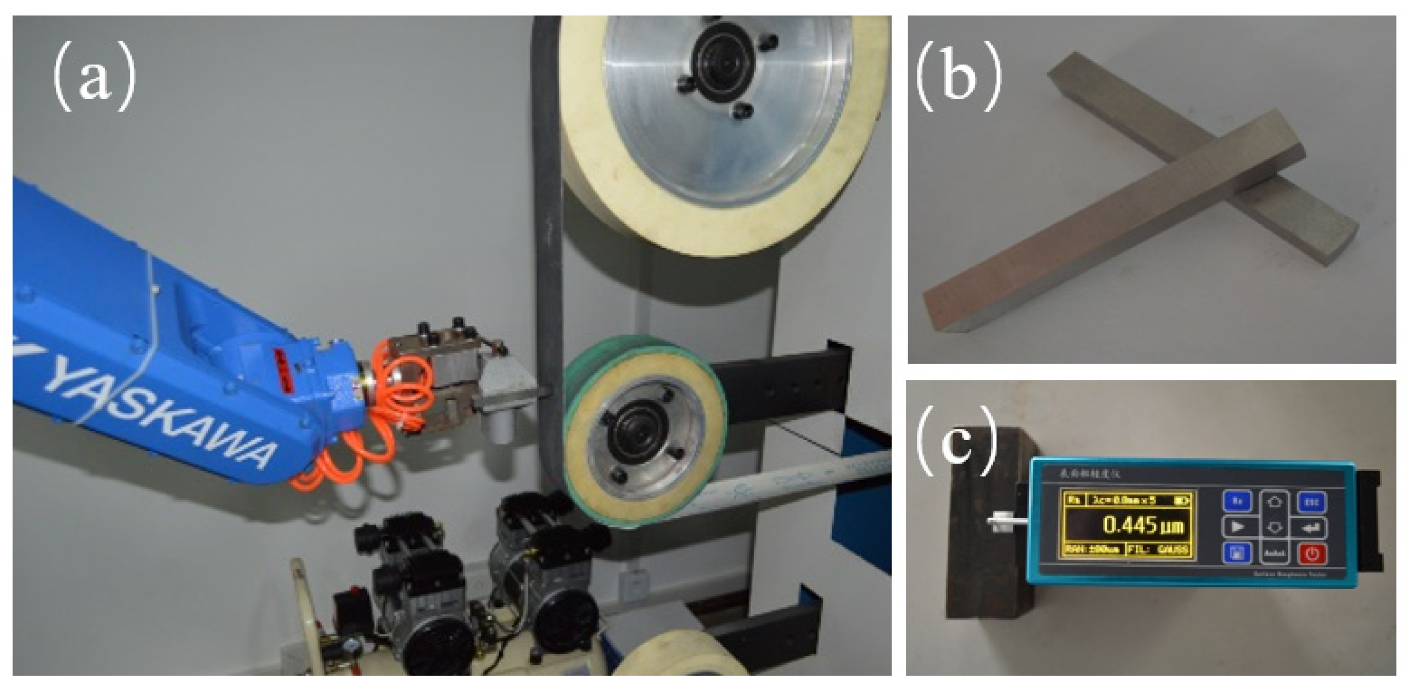
After the determination of experimental program, all test equipment and samples are prepared shown in Figure 4. The actual grinding experiment can be seen in Figure 4a. TR210 roughness tester, as shown in Figure 4c, is used in the measurement, which can measure the surface roughness of workpiece of 45 steel shown in Figure 4b. Precision electronic balance is applied to measure the weight of workpiece to calculate MRR. Belt linear speed can be adjusted continuously by using an operating inverter. Contact force is determined by using a pressure tester. Since the workpiece is mounted on the robot arm end, the feed speed of workpiece is set by the robot control system using its programming teaching box.

3.2. Single-Factor Experiment

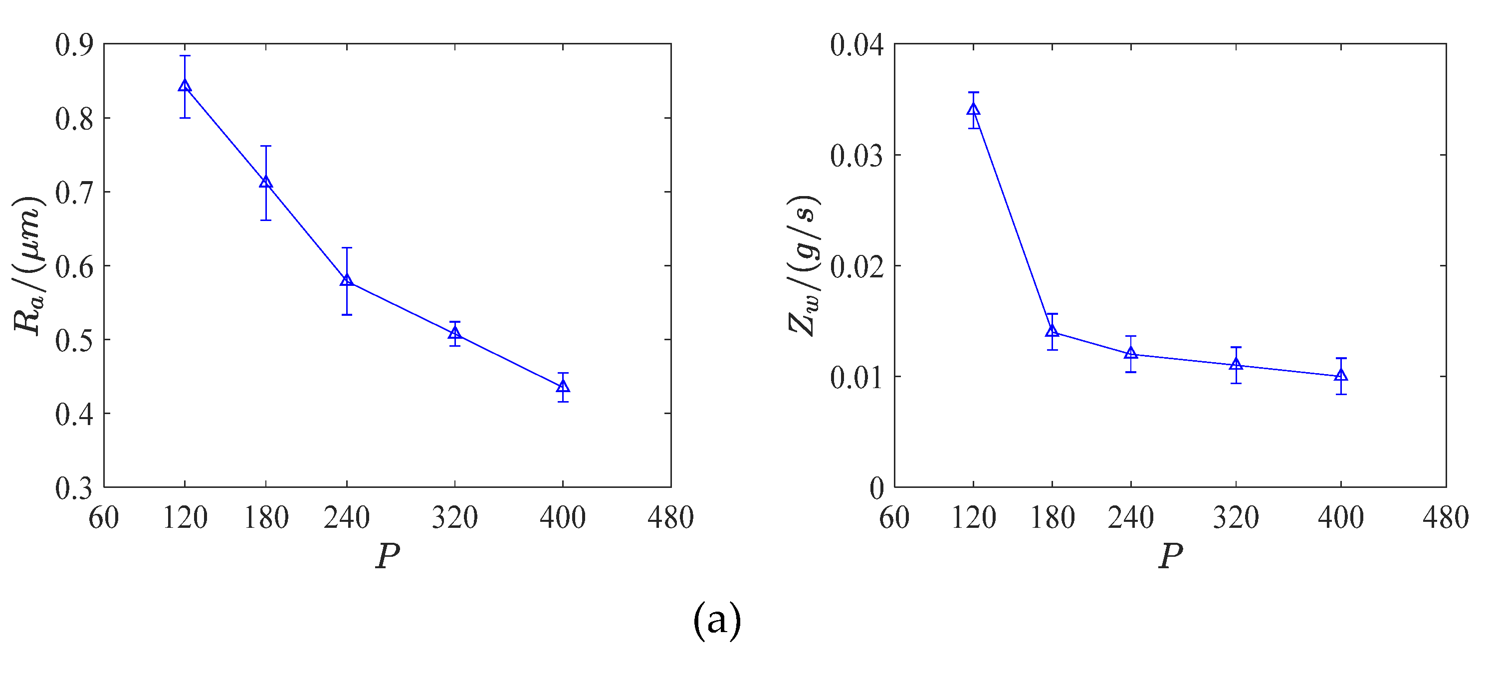
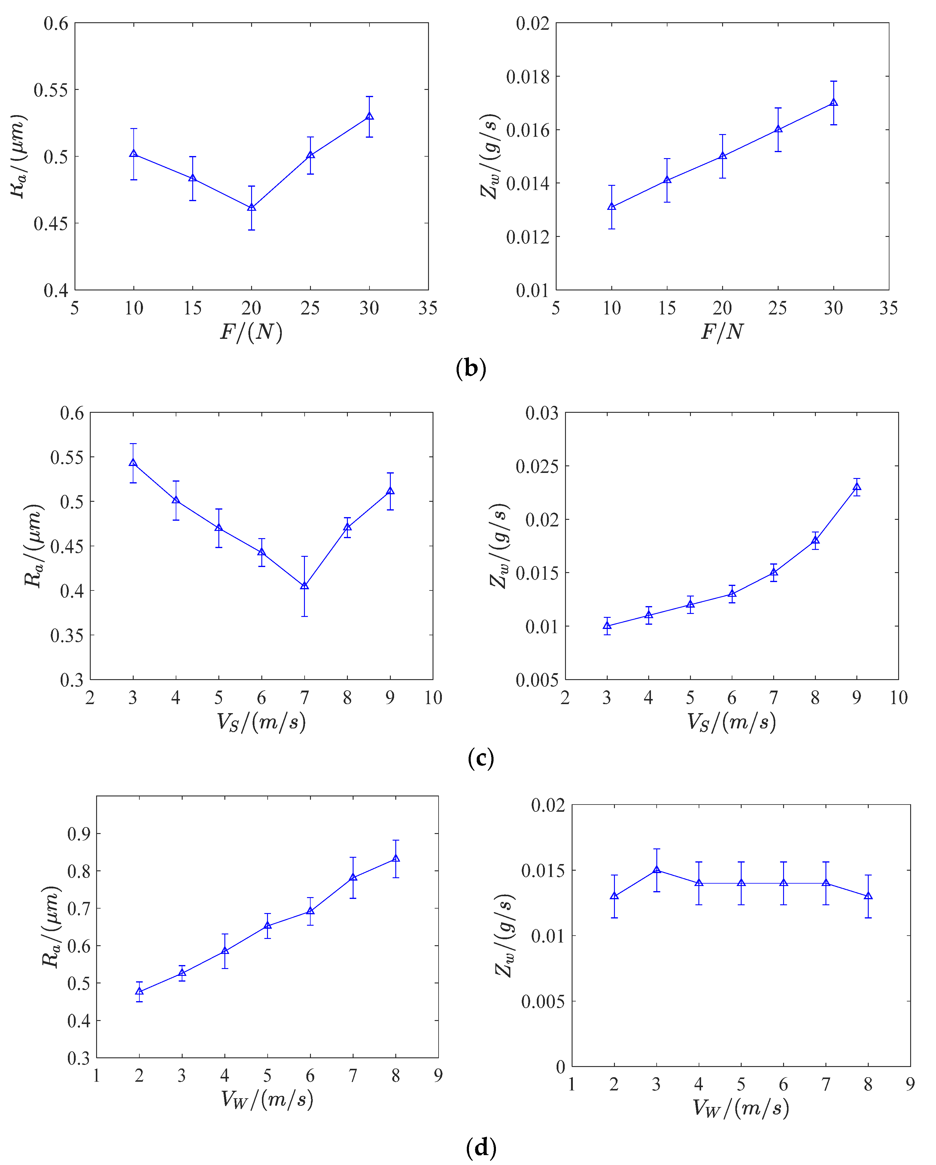
In the single-factor experiment, key grinding parameters such as abrasive size (P), contact force (F), belt linear speed (VS), and feed speed (VW) were considered as control factors. It was found that the abrasive size was the most significant factor in both surface roughness (Ra) and MRR (Zw). In Figure 5a, it shows that surface roughness decreases rapidly along with the increasing of abrasive size, MRR of workpiece drops sharply when abrasive size change from 120# to 180#, then goes down gently from 180# to 400#. In Figure 5b, it suggests that surface roughness can reach the minimum value when the contact force is 20 N, MRR has an approximate linear growth trend along with belt linear speed increases. In Figure 5c, it produces the lowest surface roughness value when the belt linear speed is 7 m/s, MRR has an approximate parabolic growth trend along with contact force increases. In Figure 5d, it reveals that surface roughness increases continuously with the increase of feed speed, while MRR remains almost unchanged under the same condition.

3.3. Weighting Objective Method

The weighting objective method is selected to use in this situation by building a weighted sum of the two objectives (Ra and Zw) [21,22] to form the unified objective function Y as:
Y ( x ) = λ a R a ( x ) λ w Z w ( x )
where
λ a + λ w = 1
and
x = [ P F V s V w ] T
where λa and λw are the weighting coefficients that represent the relative importance of each criterion and reflect closely importance of objectives.
As the surface roughness and MRR are two different goals, so it is necessary to evaluate them at the same level. Generally, normalization is the best way to solve this problem as:
Y ^ ( x ) = λ a R ^ a ( x ) λ w Z ^ w ( x )
where Y ^ is the new comprehensive goal that can be seen as normalized Y . R ^ a is the normalized surface roughness and Z ^ w is normalized MRR. Since the surface roughness is more important than MRR for products, it is reasonable to set the value of weighting coefficient λa be larger than λw.
In the experiment, R a ( x 1 , x 2 , x 3 , , x n ) and Z w ( x 1 , x 2 , x 3 , , x n ) is the measured data, R ^ a ( x 1 , x 2 , x 3 , , x n ) and Z ^ w ( x 1 , x 2 , x 3 , , x n ) is normalized. The normalized method can be described as follows:
R ^ a ( x i ) = R a ( x i ) min R a ( x 1 , x 2 , x 3 , , x n ) max R a ( x 1 , x 2 , x 3 , , x n ) min R a ( x 1 , x 2 , x 3 , , x n ) ( i = 1 , 2 n )
Z ^ w ( x i ) = Z w ( x i ) min Z w ( x 1 , x 2 , x 3 , , x n ) max Z w ( x 1 , x 2 , x 3 , , x n ) min Z w ( x 1 , x 2 , x 3 , , x n ) ( i = 1 , 2 n )

3.4. Central Composite Design (CCD)

A response surface methodology was applied to optimize the grinding conditions of 45 steel. A three-level central composite design (CCD) with three factors was selected to examine the comprehensive goal, and an experimental design can be seen in Table 4. The factors of abrasive size (X1), grinding contact force (X2), belt linear speed (X3), and feed speed (X4) were chosen as independent variables. When the value of weighting factor λa and λw were selected as 0.6 and 0.4, respectively, the coded and real values of abrasive size (X1) were 0 for 240#, 1 for 320#, and 2 for 400#, those for contact force (X2) were 0 for 15 N, 1 for 20 N, 2 for 25 N, those for belt linear speed (X3) were 0 for 6 m/s, 1 for 7 m/s, 2 for 8 m/s, and those for feed speed (X4) were 0 for 2 mm/s, 1 for 3 mm/s, 2 for 4 mm/s. We obtained similar interpretations referring to the above when the weighting factor λa and λw were selected as other values. Regression analysis was done on the data obtained by triplicate analysis for each dependent variable using design-expert software (Table 5). Response surface analysis was also applied to the data from CCD for modeling and prediction of optimum grinding contact force, belt linear speed, and feed speed.

3.5. Regression Analysis of Experimental Results

In the process of grinding, since the comprehensive goal of Y ^ prediction model is nonlinear, the fitting was done by using a second-order model for each response [23]. The mathematical relationship between the independent variables can be expressed by:
Y R = β 0 + i = 1 n β i X i + i = 1 n β i i X i 2 + i = 1 n 1 j = 2 j > i n β i j X i X j
where YR is the predicted response (comprehensive goal Y ^ ) and Xi represents the independent variables (abrasive size, contact force, belt linear speed, feed speed) that are known for each experimental run. The parameter β0 is the model constant, βi is the linear coefficient, βii is the quadratic coefficients, and βij is the cross coefficients.
The Model F-value of 26.58 implies that the model is significant. There is only a 0.01% chance that a “Model F-Value” this large could occur due to noise. Values of “Prob > F” less than 0.0500 indicate model terms are significant. In this case, X1, X2, X3, X4, X1X2, X1X3, X12, X22, X32 are significant model terms. The “Lack of Fit p-value” of 10.06 indicates that the LOF is significant. The value of R2 is 0.9612 shows that 96.12% of experimental data confirm the compatibility with the data predicted by the model. The “Pred R2” of 0.8676 is in reasonable agreement with the “Adj R2” of 0.9251. “Adeq Precision” measures the signal to noise ratio. A ratio greater than 4 is desirable. The ratio of 22.646 indicates an adequate signal. This model can be used to navigate the design space (Table 6).
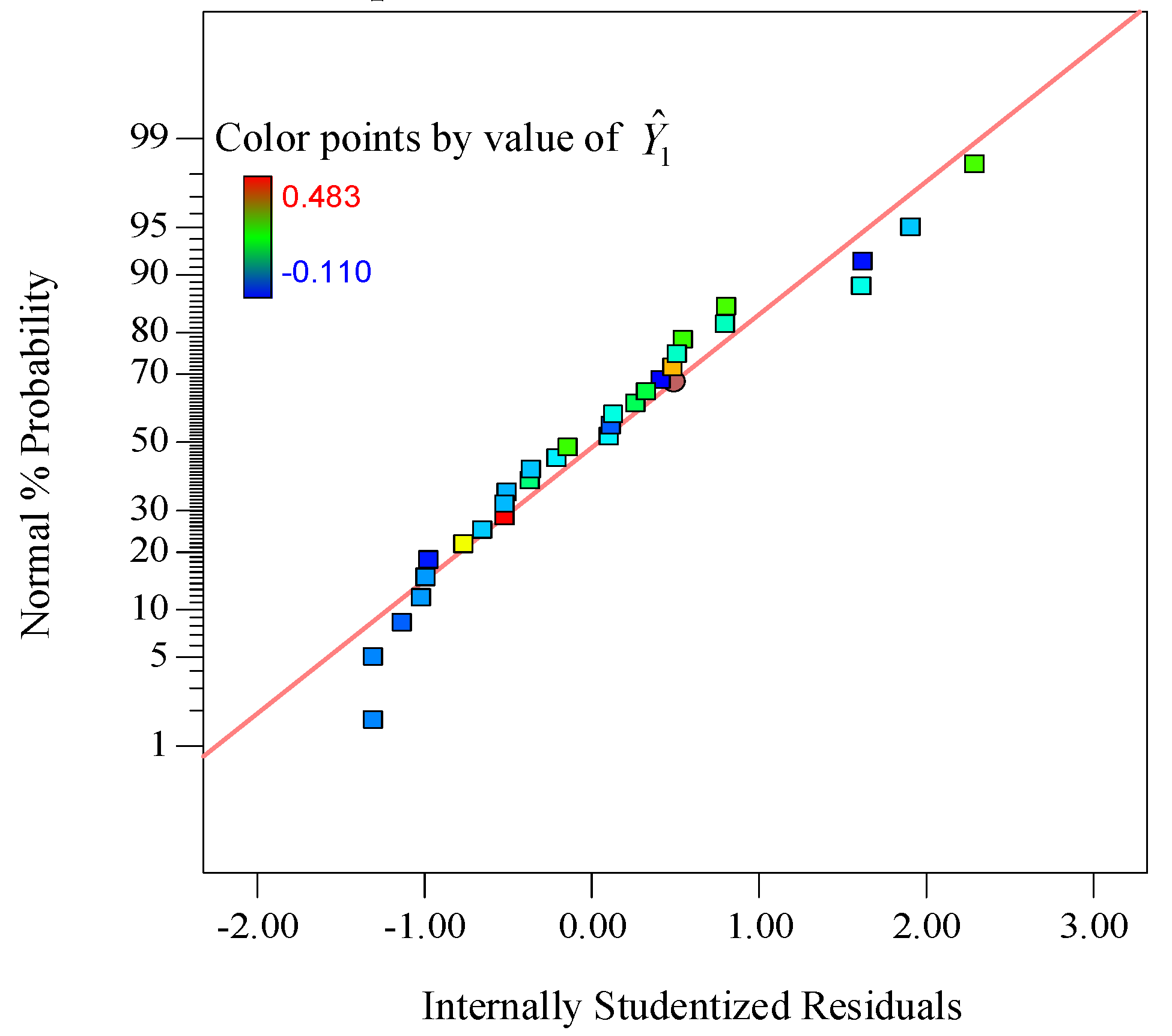
The normal plot of residuals (as shown in Figure 6) shows that the errors are distributed normally. Figure 7 also shows each experimental value matches well with its predicted value.
After conducting the experiment, the obtained data were modeled and a quadratic equation for comprehensive goal Y ^ 1 was achieved as follows:
Y ^ 1 = 6.34756 + 0.00124309 X 1 0.15942 X 2 1.35614 X 3 + 0.21733 X 4 + 0.0000954688 X 1 X 2 + 0.000349219 X 1 X 3 0.000130469 X 1 X 4 0.00321250 X 2 X 3 0.00283750 X 2 X 4 + 0.00256250 X 3 X 4 0.0000100836 X 1 2 + 0.00349860 X 2 2 + 0.088965 X 3 2 0.014035 X 4 2
Similarly, the regression model for comprehensive goal of Y ^ 2 , Y ^ 3 and Y ^ 4 were established as follows:
Y ^ 2 = 7.92318 0.00130370 X 1 0.19631 X 2 1.61488 X 3 + 0.34007 X 4 + 0.000101719 X 1 X 2 + 0.000371094 X 1 X 3 0.000169531 X 1 X 4 0.00191250 X 2 X 3 0.00286250 X 2 X 4 0.00106250 X 3 X 4 0.00000704907 X 1 2 + 0.00417544 X 2 2 + 0.10639 X 3 2 0.028114 X 4 2 Y ^ 3 = 9.47886 0.00384649 X 1 0.23318 X 2 1.86806 X 3 + 0.46160 X 4 + 0.000107813 X 1 X 2 + 0.000390625 X 1 X 3 0.000209375 X 1 X 4 0.000625 X 2 X 3 0.002925 X 2 X 4 0.0045 X 3 X 4 0.00000398986 X 1 2 + 0.0048586 X 2 2 + 0.12346 X 3 2 0.042035 X 4 2 Y ^ 4 = 11.04075 0.00639606 X 1 0.27025 X 2 2.12170 X 3 + 0.58284 X 4 + 0.000113750 X 1 X 2 + 0.000410937 X 1 X 3 0.000246875 X 1 X 4 0.000675 X 2 X 3 0.00295 X 2 X 4 0.008125 X 3 X 4 0.000000929276 X 1 2 + 0.00554211 X 2 2 + 0.14055 X 3 2 0.055947 X 4 2

4. Grinding Parameters Optimization

As the optimization procedure is analogous for different surface roughness weighting coefficients, it is representative to select one to be optimized. In the following section, as an optimization example, the optimal value of each parameter is tried to minimize the comprehensive goal Y ^ 1 when the surface roughness weighting coefficient λa = 0.6 and MRR weighting coefficient λw = 0.4.
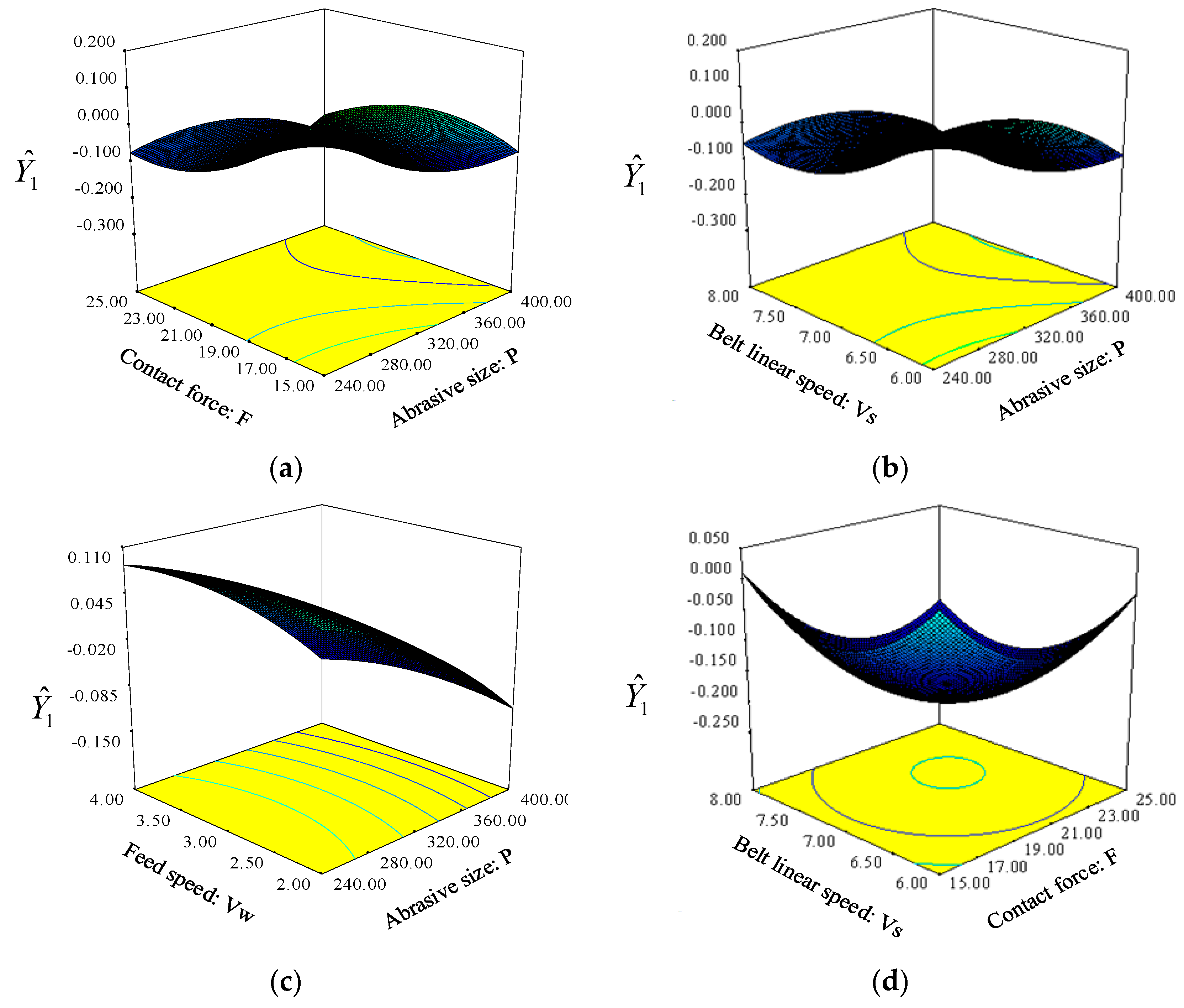
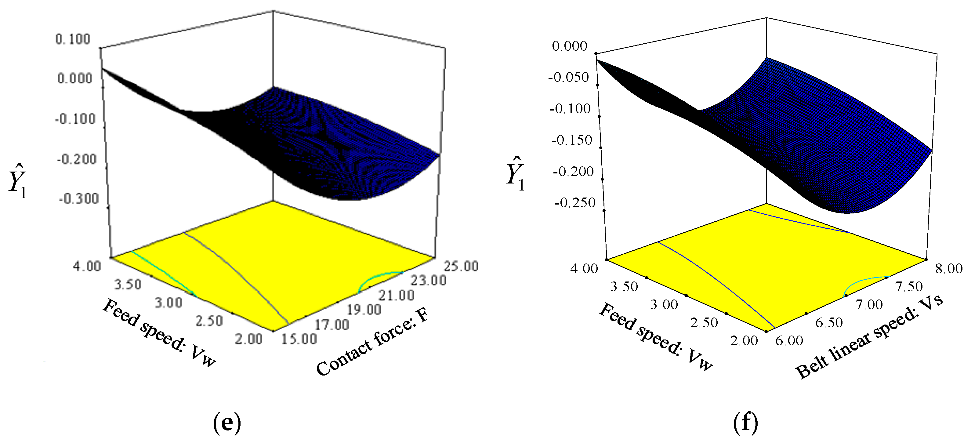
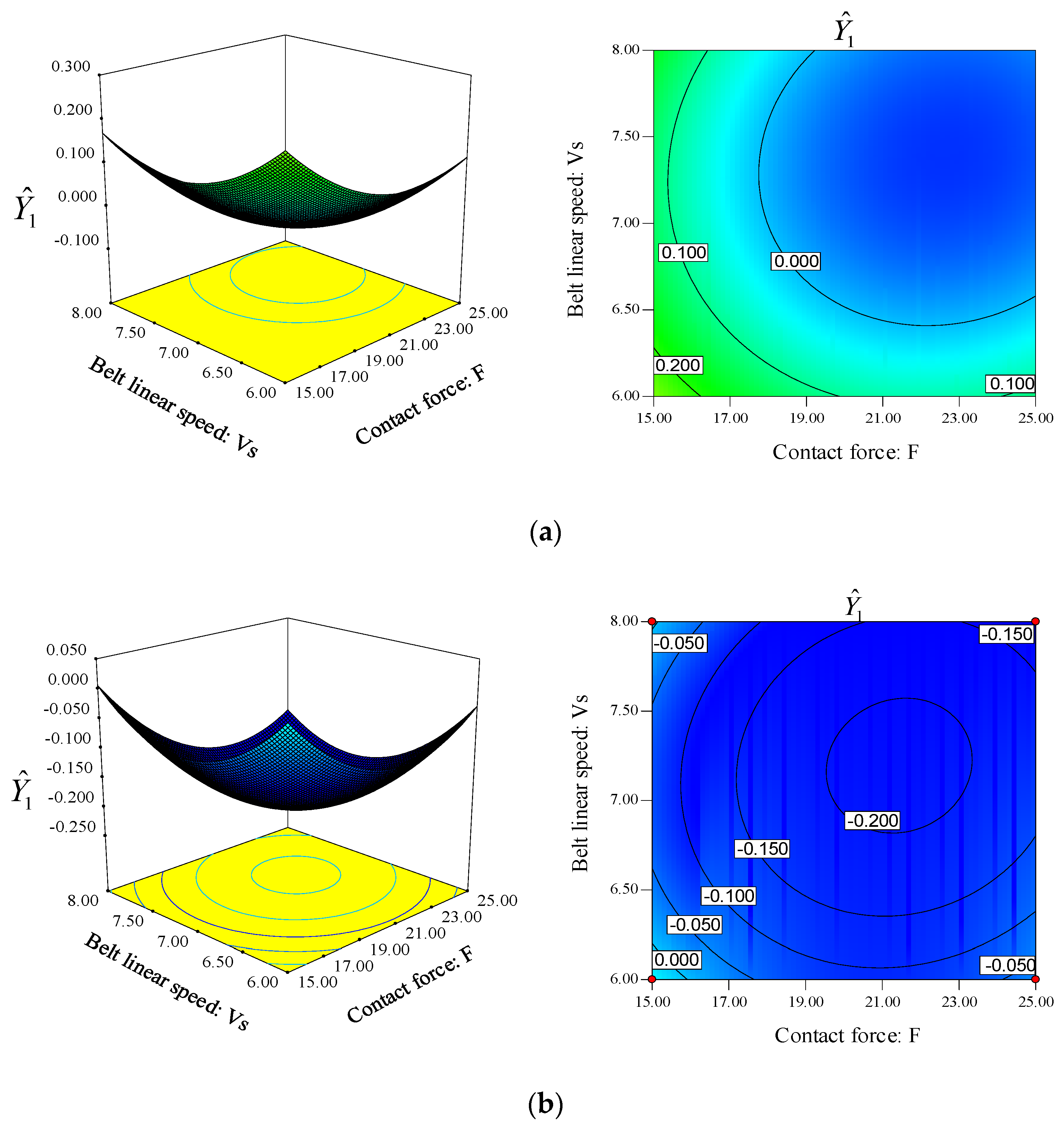
The optimal value of each grinding parameter was determined by a Y ^ 1 prediction model using design-expert software and obtained from Figure 8. The grinding parameters for grinding are abrasive size of 398.16#, contact force of 21.35 N, belt linear speed of 7.13 m/s and feed speed of 2.00 mm/s. But the abrasive size of 398.16# doesn’t exist in practical use. Therefore, the abrasive size of 320# and 400# were the only a limited selection of abrasive sizes, they were considered to replace 398.16#. In addition, the grinding belt was replaced regularly. The respond surface of abrasive size for 320# and 400# is established, as shown in Figure 9, it shows the comprehensive goal Y ^ 1 minimum value is −0.022 when the abrasive size is 320#, and which is much larger than that of −0.210 when the abrasive size is 400#. So the optimum grinding parameters are abrasive size of 400#, contact force of 21.35 N, belt linear speed of 7.13 m/s, and feed speed of 2.00 mm/s.

5. Experimental Verification and Analysis

The optimized parameters were used in the new experiment to verify that the method is effective. The result is shown in Table 7. No.18 of the above CCD experiment achieved the minimum value of 0.390 μm, so it was suitably chosen as the comparison group.
From Table 7, compared with reference group, when λa is 0.6 and 0.7, the mean value of surface roughness went down by 2.05% and 4.62% respectively, and the mean value of MRR of both went up 11.11% to 0.020 g/s; when λa is 0.8 and 0.9, the mean value of surface roughness went down by 10.51% and 14.87% respectively, and the mean value of MRR of both went up 5.55% to 0.019 g/s. In addition, the error ranges in the values of surface roughness and MRR of both groups are estimated to be −0.05 to 0.05, and −0.001 to 0.001 respectively.These results reveal a trend that the optimized value of both surface roughness and MRR decrease along with the increase of surface roughness weighting coefficient.
Furthermore, 2D profiles of the workpiece surfaces from optimized and unoptimized group are extracted by using laser scanning confocal microscope (OLYMPUS, OSL4100), it shows that the surface quality of 45 steel from optimization group shown in Figure 10a,b, has significantly improved compared with that obtained from the unoptimized group, shown in Figure 10c–e. The experiment results show the prediction model is reliable, that is to say, this method is effective for optimizing grinding parameters.

6. Conclusions

This study focuses on the experiment of grinding parameters that uses two performance measures, including surface roughness and workpiece MRR. The influences of abrasive size, contact force, belt linear speed as well as feed speed were investigated for achieving 45 steel grinding with high surface quality and high MRR. The two objectives including minimization of the surface roughness and maximization of the MRR are converted to one comprehensive goal by using the weighting objective method. The CCD and RSM were used to facilitate the understanding of the deep influence of grinding parameters. The optimum grinding conditions were obtained under different grinding goals. Based on the results and comparisons, it is observed that the approach proposed in this work has enhanced the surface grinding performance and optimized the grinding parameters in the surface grinding process. The knowledge derived from this study would be useful for expanding practical use of grinding parameters optimization technology.

Author Contributions

F.L. devised the research plan. Y.X. and Z.Z. performed the research and wrote the initial manuscript. W.S. helped Z.Z. do the research. Y.X. edited the manuscript and made the final figures. F.L. and J.X. provided technical help over the course of the research. All authors have read and agreed to the published version of the manuscript.

Funding

This research was funded by Laser Manufacturing and Additive Manufacturing Project of National Key Research and Development Program of China (Grant No. 2018YFB1108000), National Natural Science Foundation of China (Grant No. U1609209), and Wenzhou Municipal Key Science and Research Program (Grant No. ZG2017003).

Conflicts of Interest

The authors declare no conflict of interest.

References

  1. Pang, G.P.; Qi, X.Z.; Ma, Q.Y. Surface roughness and roundness of bearing raceway machined by floating abrasive polishing and their effects on bearing’s running noise. Chin. J. Mech. Eng. 2014, 27, 543–550. [Google Scholar] [CrossRef]
  2. Song, J.F.; Yao, Y.X. Material removal model considering influence of curvature radius in bonnet polishing convex surface. Chin. J. Mech. Eng. 2015, 28, 1109–1116. [Google Scholar] [CrossRef]
  3. Song, J.F.; Yao, Y.X.; Xie, D.G. Effects of polishing parameters on material removal for curved optical glasses in bonnet polishing. Chin. J. Mech. Eng. 2008, 21, 29–33. [Google Scholar] [CrossRef]
  4. Liu, Y.F.; Zhao, H.; Jing, J.T. Research on material removal rate in rotary ultrasonic grinding machining. Int. J. Nanomanuf. 2011, 7, 158–168. [Google Scholar] [CrossRef]
  5. Wu, S.H.; Kazerounian, K.; Gan, Z.X. A simulation platform for optimal selection of robotic belt grinding system parameters. Int. J. Adv. Manuf. Technol. 2013, 64, 447–458. [Google Scholar] [CrossRef]
  6. Ho, L.T.; Cheung, C.F.; Blunt, L. An investigation of factors affecting and optimizing material removal rate in computer controlled ultra-precision polishing. In Key Engineering Materials; Trans Tech Publications: Zurich, Switzerland, 2015; Volume 625, pp. 446–452. [Google Scholar]
  7. Zhao, T.; Shi, Y.Y.; Lin, X.J. Surface roughness prediction and parameters optimization in grinding and polishing process for IBR of aero-engine. Int. J. Adv. Manuf. Technol. 2014, 74, 653–663. [Google Scholar] [CrossRef]
  8. Yong, Y.W.; Kulkarni, S.; Rys, M. Development of a surface roughness model in end milling of nHAP using PCD insert. Ceram. Int. 2012, 38, 6865–6871. [Google Scholar] [CrossRef]
  9. Periyasamy, S.; Aravind, M.; Vivek, D. Optimization of surface grinding process parameters for minimum surface roughness in AISI 1080 using response surface methodology. Adv. Mater. Res. 2014, 984, 118–123. [Google Scholar] [CrossRef]
  10. Abdur-RASHEED, A.; Konneh, M. Optimization of Precision Grinding Parameters of Silicon for Surface Roughness Based on Taguchi Method. In Advanced Materials Research; Trans Tech Publications: Zurich, Switzerland, 2011; Volume 264, pp. 997–1002. [Google Scholar]
  11. Zheng, X.F.; Yuan, J.L.; Wen, D.H. Parameters optimization on the lapping process of 9Cr18 with Taguchi method. In Key Engineering Materials; Trans Tech Publications: Zurich, Switzerland, 2008; Volume 359, pp. 158–161. [Google Scholar]
  12. Yuan, J.L.; Lv, B.H.; Zhou, Z.Z. Parameters optimization on the lapping process for advanced ceramics by applying Taguchi method. Mater. Sci. Forum. Trans. Tech. Publ. 2006, 532, 488–491. [Google Scholar] [CrossRef]
  13. Guven, O. Application of the Taguchi method for parameter optimization of the surface grinding process. Mater. Test. 2015, 57, 43–48. [Google Scholar] [CrossRef]
  14. Gopal, A.V.; Rao, P.V. Selection of optimum conditions for maximum material removal rate with surface finish and damage as constraints in SiC grinding. Int. J. Mach. Tools Manuf. 2003, 43, 1327–1336. [Google Scholar] [CrossRef]
  15. Ting, T.O.; Lee, T.S.; Htay, T. Performance analysis of grinding process via particle swarm optimization. In Proceedings of the Sixth International Conference on Computational Intelligence and Multimedia Applications (ICCIMA’05), Las Vegas, NV, USA, 16–18 August 2005; pp. 92–97. [Google Scholar]
  16. Kumar, M.; Singh, S.; Goyal, K. To study the effect of grinding parameters on surface roughness and material removal rate of cylindrical grinding of heat treated en 47 steel. J. Mech. Eng. 2016, 45, 81–88. [Google Scholar] [CrossRef] [Green Version]
  17. Pai, D.; Rao, S.; D’souza, R. Application of response surface methodology and enhanced non-dominated sorting genetic algorithm for optimisation of grinding process. Procedia Eng. 2013, 64, 1199–1208. [Google Scholar] [CrossRef] [Green Version]
  18. Kumar, P.; Kumar, A.K.; Singh, B. Optimization of process parameters in surface grinding using response surface methodology. Int. J. Res. Mech. Eng. Technol. 2013, 3, 245–252. [Google Scholar]
  19. Sedighi, M.; Afshari, D. Creep feed grinding optimization by an integrated GA-NN system. J. Intell. Manuf. 2010, 21, 657–663. [Google Scholar] [CrossRef]
  20. Lee, P.H.; Chung, H.; Lee, S.W. Optimization of micro-grinding process with compressed air using response surface methodology. Proc. Inst. Mech. Eng. Part B J. Eng. Manuf. 2011, 225, 2040–2050. [Google Scholar] [CrossRef]
  21. Xiang, J.W.; Yang, L.F.; Li, S.P. Experimental investigation of the basecutter for minitype sugarcane harvester. Trans. Chin. Soc. Agric. Eng. 2007, 23, 158–163. [Google Scholar]
  22. Oliveira, L.S.D.; Saramago, S.F. Multiobjective optimization techniques applied to engineering problems. J. Braz. Soc. Mech. Sci. Eng. 2010, 32, 94–105. [Google Scholar] [CrossRef] [Green Version]
  23. Myers, R.H.; Montgomery, D.C.; Anderson-cook, C.M. Response Surface Methodology: Process and Product Optimization Using Designed Experiments; John Wiley & Sons: Hoboken, NJ, USA, 2016. [Google Scholar]
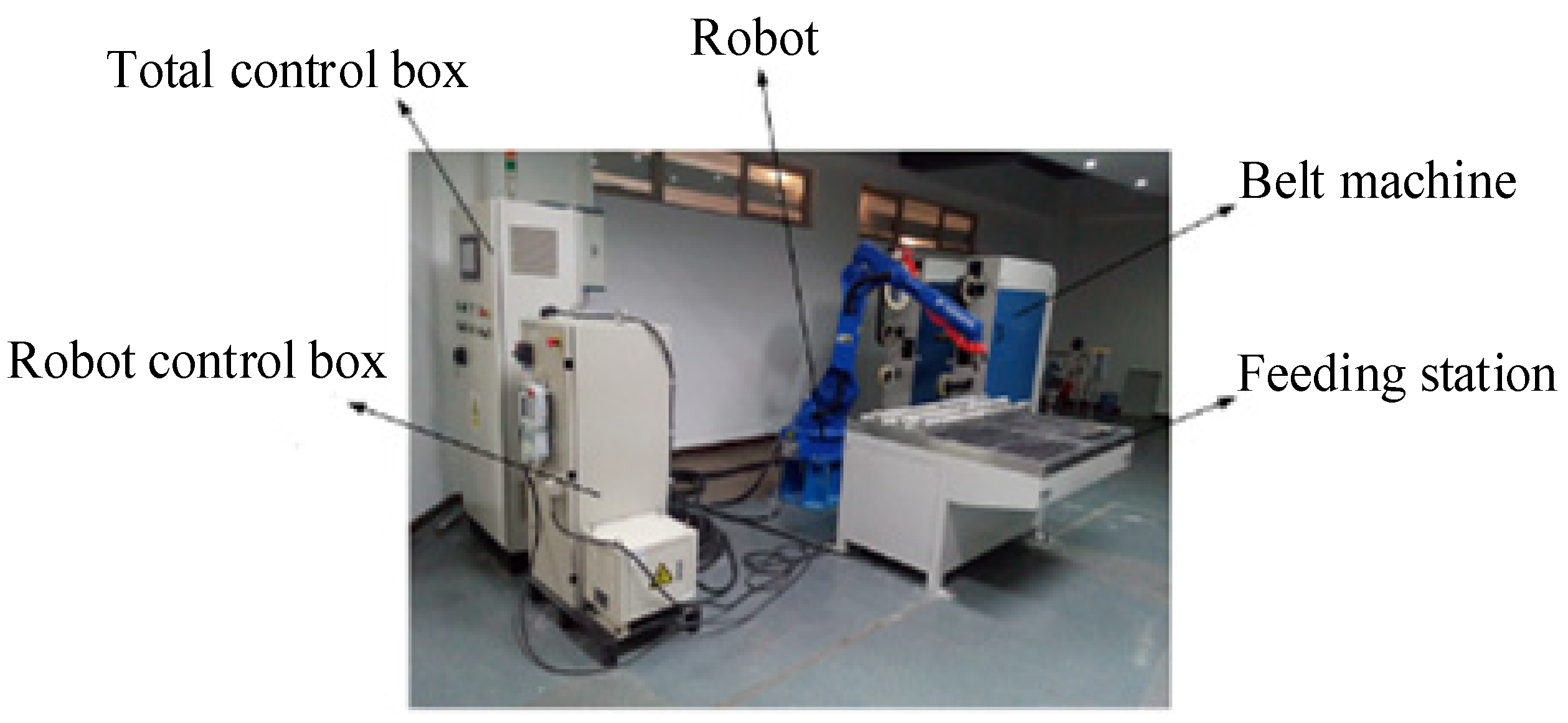
Figure 1. Robot belt grinding system.
Applsci 10 06314 g001
Figure 2. Belt transmission and tensioning system.
Applsci 10 06314 g002
Figure 3. (a) schematic depiction of the abrasive belt grinding; (b) local schematic of workpiece and belt polishing.
Applsci 10 06314 g003
Figure 4. (a) Grinding experiment; (b) Workpiece of 45 steel; (c) TR210 roughness tester.
Applsci 10 06314 g004
Figure 5. Single-factor experiment. (a) Abrasive size (Ra: roughness; Zw: MRR; P: abrasive size); (b) Contact force (Ra: roughness; Zw: MRR; F/N: contact force); (c) Belt linear speed (Ra: roughness; Zw: MRR; Vs: belt linear speed); (d) Feed speed (Ra: roughness; Zw: MRR; VW: feed speed).
Applsci 10 06314 g005aApplsci 10 06314 g005b
Figure 6. Normal plot of residuals.
Applsci 10 06314 g006
Figure 7. Predicted vs. actual.
Applsci 10 06314 g007
Figure 8. Response surfaces for the optimal value of each grinding parameter. (a) VS = 7.13 m/s, VW = 2.00 mm/s; (b) F = 21.35 N, VW = 2.00 mm/s; (c) F = 21.35 N, VS = 7.13 m/s; (d) P = 398.16#, VW = 2.00 mm/s; (e) P = 398.16#, VS = 7.13 m/s; (f) P = 398.16#, F = 21.35 N.
Applsci 10 06314 g008aApplsci 10 06314 g008b
Figure 9. Respond surfaces in two different abrasive sizes. (a) P = 320#, VW = 2.00 mm/s; (b) P = 400#, VW = 2.00 mm/s.
Applsci 10 06314 g009
Figure 10. 2D profiles of the workpiece surfaces from optimized and unoptimized group. Optimized group: (a) Ra = 0.332 ± 0.050 μm, (b) Ra = 0.382 ± 0.050 μm; Unoptimized group: (c) Ra = 0.550 ± 0.050 μm, (d) Ra = 0.750 ± 0.050 μm, (e) Ra = 0.850 ± 0.050 μm.
Applsci 10 06314 g010
Table 1. Chemical composition of 45 steel.
Element TypeCSiMnCr
Percentage (%)0.42–0.500.17–0.370.5–0.80≤0.25
Element typeNiCuFe
Percentage (%)≤0.30≤0.25remaining
Table 2. Workpiece characteristics before belt grinding.
Workpiece Characteristics
Workpiece material45 Steel
Superficial hardness of workpiece<HRC28
Initial roughness5–10 μm
Size of the grinding surface10 × 10 mm
Table 3. Grinding condition.
Material of Driving and Driven WheelsPolyurethane
Single grinding time20 s
Perimeter and width of belt(4000 × 90) mm
Grinding typeDry grinding
Robot typeYaskawa HP-20D
Table 4. Level of factors distribution of grinding (λa = 0.6; λa = 0.7; λa = 0.8; λa = 0.9).
ParameterUnitCodeLevel
012
Abrasive size (P)#X1240#320#400#
Contact force (F)NX2152025
Belt linear speed (Vs)m/sX3678
Feed speed (Vw)mm/sX4234
Table 5. Central experiment design table and experiment results.
No.ParameterResultsλa = 0.6λa = 0.7λa = 0.8λa = 0.9
P F V S   V W   R a R ^ a Z w Z ^ w Y ^ 1 Y ^ 2 Y ^ 3 Y ^ 4
124015620.7090.7690.020.3330.3280.4380.5480.658
240015620.4800.2170.0180.2500.0300.0770.1230.170
324025620.6230.5610.0240.5000.1370.2430.3490.455
440025620.4330.1040.0190.292−0.054−0.0150.0250.064
524015820.6570.6430.0220.4170.2190.3250.4310.537
640015820.4790.2140.0200.333−0.0050.0500.1050.160
724025820.6000.5060.0361.000−0.0960.0540.2050.355
840025820.4640.1780.0250.542−0.110−0.0380.0340.106
924015640.8051.0000.0190.2920.4830.6130.7420.871
1040015640.4940.2510.0120.0000.1500.1750.2000.226
1124025640.6690.6720.0230.4580.2200.3330.4460.559
1240025640.4760.2070.0190.2920.0080.0580.1070.157
1324015840.7430.8510.0200.3330.3770.4950.6140.732
1440015840.4930.2480.0140.0830.1160.1490.1820.215
1524025840.6080.5250.0290.7080.0320.1550.2790.402
1640025840.4780.2120.0230.458−0.0560.0110.0780.145
1724020730.5810.4600.0240.5000.0760.1720.2680.364
1840020730.3900.0000.0180.250−0.100−0.075−0.050−0.025
1932015730.5710.4360.0140.0830.2280.2800.3320.384
2032025730.5180.3080.0200.3330.0520.1160.1800.244
2132020630.5590.4070.0130.0420.2280.2730.3170.362
2232020830.5320.3420.0210.3750.0550.1270.1990.270
2332020720.4170.0650.0140.0830.0060.0210.0350.050
2432020740.4850.2290.0160.1670.0710.1100.1500.189
2532020730.4560.1590.0190.292−0.0210.0240.0690.114
2632020730.4570.1610.0190.292−0.0200.0260.0710.116
2732020730.4600.1690.0200.333−0.0320.0180.0680.118
2832020730.4620.1730.0180.2500.0040.0460.0890.131
2932020730.4600.1690.0200.333−0.0320.0180.0680.118
3032020730.4690.1900.0190.292−0.0020.0460.0940.142
(Ra unit: μm; Zw unit: g/s).
Table 6. ANOVA for the response surface quadratic model of Y ^ 1 .
Source Y ^ 1 Y ^ 2
Sum of SquaresdfMean SquareF Valuep-Value Prob > FSum of SquaresdfMean SquareF Valuep-Value Prob > F
Model0.60140.04326.58<0.00010.78140.05543.71<0.0001
X1P0.1810.18111.68<0.00010.3310.33260.20<0.0001
X2F0.1810.18111.18<0.00010.1610.16124.49<0.0001
X3VS0.05510.05534.45<0.00010.04210.04232.96<0.0001
X4VW0.05010.05030.95<0.00010.05010.05039.07<0.0001
X1X20.02310.02314.520.00170.02610.02620.910.0004
X1X30.01210.0127.770.01380.01410.01411.130.0045
X1X40.00174310.0017431.090.31410.00294310.0029432.320.1483
X2X30.00412810.0041282.570.12980.00146310.0014631.150.2995
X2X40.00322110.0032212.000.17720.00327810.0032782.590.1286
X3X40.000105110.00010510.0650.80160.0000180610.000018060.0140.9065
X120.01110.0116.720.02040.00527310.0052734.160.0594
X22,0.02010.02012.340.00310.02810.02822.280.0003
X320.02110.02112.770.00280.02910.02923.140.0002
X420.000510410.00051040.320.58130.00204810.0020481.620.2230
Residual0.024150.001606 0.019150.001267
Lack of Fit0.023100.00229610.060.01000.018100.00181510.660.0088
Pure Error0.00114150.0002282 0.000851350.0001703
Cor Total0.6229 0.7929
SD = 0.040, Mean = 0.076, C.V.% = 52.46, PRESS = 0.082,
R2 = 0.9612, Adj R2 = 0.9251, Pred R2 = 0.9676,
Adeq Precision = 22.646
SD = 0.036, Mean = 0.14, C.V.% = 24.69, PRESS = 0.063,
R2 = 0.9761, Adj R2 = 0.9537, Pred R2 = 0.9204,
Adeq Precision =29.293
Source Y ^ 3 Y ^ 4
Sum of SquaresdfMean SquareF Valuep-Value Prob > FSum of SquaresdfMean SquareF Valuep-Value Prob > F
Model1.03140.07365.63<0.00011.35140.09682.31<0.0001
X1P0.5310.53471.77<0.00010.7710.77656.31<0.0001
X2F0.1410.14123.37<0.00010.1210.12102.20<0.0001
X3VS0.03010.03026.540.00010.02010.02017.120.0009
X4VW0.04910.04944.28<0.00010.04910.04942.11<0.0001
X1X20.03010.03026.670.00010.03310.03328.35<0.0001
X1X30.01610.01614.000.00200.01710.01714.800.0016
X1X40.00448910.0044894.020.06330.00624110.0062415.340.0354
X2X30.000156310.00015630.140.71350.000182310.00018230.160.6984
X2X40.00342210.0034223.070.10030.00348110.0034812.980.1048
X3X40.000324010.00032400.290.59790.00105610.0010560.900.3567
X120.00168910.0016891.510.23740.0000916410.000091640.0780.7832
X220.03810.03834.26<0.00010.05010.05042.57<0.0001
X320.03910.03935.40<0.00010.05110.05143.81<0.0001
X420.00457810.0045784.100.06100.00811010.0081106.940.0188
Residual0.017150.001116 0.018150.001168
Lack of Fit0.016100.00160411.570.00730.017100.00169213.990.0047
Pure Error0.000693550.0001387 0.000604850.0001210
Cor Total1.0429 1.3629
SD = 0.033, Mean = 0.21, C.V.% = 15.76, PRESS = 0.063,
R2 = 0.9839, Adj R2 = 0.9689, Pred R2 = 0.9397,
Adeq Precision = 35.244
SD = 0.034, Mean = 0.28, C.V.% = 12.22, PRESS = 0.082,
R2 = 0.9872, Adj R2 = 0.9752, Pred R2 = 0.9395,
Adeq Precision = 38.371
df—degrees of freedom, CV—coefficient of variation, F—Fisher’s ratio, p—probability.
Table 7. Comparison of optimization results by using weighting objectives method and response surface methodology (RSM).
Resultλa[P, F, VS, VW]RaError of RaZwError of ZwIncrease Rate (%)
RaZw
Reference group/[400#, 20.00 N, 7.00 m/s, 3.00 mm/s]0.390±0.0500.018±0.001//
Optimized group0.6[400#, 21.35 N, 7.13 m/s, 2.00 mm/s]0.382±0.0500.020±0.001−2.0511.11
0.7[400#, 20.93 N, 7.09 m/s, 2.00 mm/s]0.372±0.0500.020±0.001−4.6211.11
0.8[400#, 20.60 N, 7.02 m/s, 2.00 mm/s]0.341±0.0500.019±0.001−10.515.55
0.9[400#, 20.38 N, 6.97 m/s, 2.00 mm/s]0.332±0.0500.019±0.001−14.875.55
(Ra unit: μm; Zw unit: g/s).