FAU-Net: Fixup Initialization Channel Attention Neural Network for Complex Blood Vessel Segmentation

Abstract

Medical image segmentation based on deep learning is a central research issue in the field of computer vision. Many existing segmentation networks can achieve accurate segmentation using fewer data sets. However, they have disadvantages such as poor network flexibility and do not adequately consider the interdependence between feature channels. In response to these problems, this paper proposes a new de-normalized channel attention network, which uses an improved de-normalized residual block structure and a new channel attention module in the network for the segmentation of sophisticated vessels. The de-normalized network sends the extracted rough features to the channel attention network. The channel attention module can explicitly model the interdependence between channels and pay attention to the correlation with crucial information in multiple feature channels. It can focus on the channels with the most association with vital information among multiple feature channels, and get more detailed feature results. Experimental results show that the network proposed in this paper is feasible, is robust, can accurately segment blood vessels, and is particularly suitable for complex blood vessel structures. Finally, we compared and verified the network proposed in this paper with the state-of-the-art network and obtained better experimental results.

1. Introduction

Medical images have multiple modalities, such as Magnetic Resonance Angiography (MRA), Computed Tomography Angiography (CTA), Positron Emission Tomography (PET), ultrasound imaging, and more. In clinical diagnosis and treatment, the segmentation technology of medical images affects the reliability of diagnosis results to a great extent. Moreover, medical image segmentation technology is the first step of many medical image processing technologies, such as visualization, 3d reconstruction. Therefore, its development will affect the evolution of other related technologies in medical image processing.

With the rapid development of deep learning, a large number of intelligent methods based on neural networks for medical images segmentation have emerged in recent years. Nevertheless, medical image segmentation has some limitations, including data scarcity and class imbalance [1]. To get the results we want through deep learning training, we often need many medical images as a data set. For solving the problem of sparse data sets, different data transformation or enhancement techniques are sometimes used to increase the number of available labeled samples, such as the automatic data augmentation method proposed by Google in 2018 [2], or use a patch-based approach to resolve class imbalances.

To reduce large data sets required for network training and improve the efficiency of the work, U-Net [3] was proposed, so that we can complete the network training with very few data sets and accurately segment the region of interest. However, U-Net has some defects, such as the accuracy of the model is limited by the batch size, and the correlation between the channels is not fully considered.

To address these issues, we propose an improved de-normalized residual block. It uses a new initialization method, which solves the problem of gradient explosion and gradient disappearance by properly adjusting initialization parameters at the beginning of training. During the training process, it can converge faster. The attention mechanism, because of its low model complexity, can be calculated in parallel, and the advantage of being able to obtain critical information is also increasingly used in medical image segmentation tasks. This paper proposes a new channel attention module called SCA, which can calculate the feature mapping value in each channel, to explore the correlation of channel.

The contributions of our work can be summarized as below:

(1)

We propose a de-normalized channel attention network, which consists of a new channel attention module SCA and an improved de-normalized block.

(2)

We construct two brain vascular data sets, which uses multiple angles of CTA and MRA images from various patients, called the ELE and CORO data sets, respectively. The labeling process consults brain vascular experts.

(3)

We perform experiments on the public retinal vascular data set DRIVE [4] and brain vascular data sets ELE and CORO, compare the results with the state-of-the-art methods, and obtain high accuracy. The effects of de-normalized structure on vascular segmentation were tested on DRIVE, ELE, and CORO data sets, respectively.

2. Related Work

In the past, many traditional algorithms can be used for medical image segmentation, including threshold-based segmentation [5], region-based image segmentation [6], edge detection-based segmentation [7], wavelet analysis and wavelet transform image segmentation method [8], genetic algorithm-based image segmentation [9,10], active contour model-based segmentation method [11]. However, traditional segmentation methods have some problems, such as the need for human intervention in the segmentation process, prior knowledge before segmentation, the existence of over-segmentation in segmentation, and low segmentation accuracy.

Deep learning-based methods for image segmentation have made significant achievements. Their accuracy has surpassed that of traditional methods. Jonathan Long et al. [12] proposed a fully convolutional network for semantic segmentation to classify images at the pixel level, solving the problem of semantic level image segmentation method. Based on it, Korez et al. [13] proposed a 3DFCN network structure. They optimized the spine structure segmented by the 3D FCN network using a deformation model algorithm, which further improved the accuracy of the segmentation of spinal MR images. Zhou et al. [14] combined the FCN algorithm and the majority voting algorithm to segment 19 targets in the human torso CT image. However, the results obtained by FCN are still not subtle enough. It classifies each pixel, does not adequately consider the relationship between pixels, and is not sensitive to the details in the image, so it is not suitable for the segmentation of blood vessels.

U-Net [3] is undoubtedly one of the most successful medical image segmentation methods. After the emergence of U-net, many network variants appeared. For example, Alom et al. [15] proposed a recursive residual convolutional neural network (R2U-net) based on U-net. This residual network can achieve deeper Network, R2U-net can make the network extract more features than U-Net. LadderNet [16], proposed by Zhuang, uses an improved residual block, where two convolutional layers in one block share the same weight, and LadderNet has more information flow paths than U-Net. This allows it to get more accurate segmentation results. Similar to Ladder, Khanal et al. [17] proposed a dynamic deep network, which adds a small U-net to classify the blurred areas of the image in a more refined manner, thereby achieving higher accuracy. Currently, the network with the most top performance on the DRIVE data set is IterNet [18] proposed by Li et al. Its structure is very similar to the dynamic deep network, has a u-net, and a mini u-net. And the blurred details of the blood vessel to be divided can be found from the segmented image itself. It has obtained the highest AUC value of 0.9816 on the DRIVE data set [4]. However, these networks do not fully consider the correlation of each channel, and a lot of effective information will be lost during the training process, so this paper introduces a channel attention mechanism.

In many image segmentation tasks, the attention module is introduced. For example, SeNet proposed by He et al. [19], it automatically learns the importance of each feature channel through learning, then according to the importance to enhance useful features and suppress useless for the current task. Zhang et al. [20] proposed the EncNet structure, in which the Context Encoding Module is used to capture the semantic context of the scene and selectively emphasize the category-related feature maps. Li et al. [21] proposed the Feature Pyramid Attention module (FPA) and Global Attention Up-sample module (GAU) and introduced an attention mechanism for semantic segmentation. Fu et al. [22] proposed DANet to capture frame feature dependencies in space and channel dimensions. The position attention module can learn the correlation of spatial features, and the channel attention module can model the correlation of channels.

At present, there are many attention-related state-of-the-art models for medical image segmentation, but they are quite different from the implementation of our network. For example, a medical imaging attention gate (AG) model was designed in Attention U-Net proposed by Oktay et al. [23], which can automatically learn to focus on different shapes and sizes of target structures, learn to find the pancreas. Sinha et al. [24] proposed multi-scale guided attention for medical image segmentation. It obtains global features through a multi-size strategy, and then introduces the learned global features into the attention module. Bastidas et al. [25] proposed the channel attention network, which uses two u-nets to extract the features of the visible stream and infrared stream of the input image respectively, and then extracts the features to obtain the final segmentation results through the attention mechanism. The channel attention module proposed in this paper will enhance the useful features after each up-sampling and sub-sampling.

Yet, there is a common problem with the above networks, i.e., to obtain accurate segmentation results, it often requires a lot of training time, and the segmentation efficiency of the network is very low. Arfan et al. [26] proposed a method based on artificial neural networks and fully parallel field-programmable gate arrays (FPGAs). The hardware implementation proposed by this method can effectively improve the segmentation efficiency. In our paper, in order to solve the performance problem, we use a de-normalization method, which can greatly reduce training time.

3. Methods

3.1. Fixup Initialization Channel Attention Neural Network

Our de-normalized channel attention network follows the basic encoder-decoder structure of U-net. Its feature fusion method is to stitch the features together in the channel dimension to form a more “thick” feature. We want to be able to extract more elaborated features, so we adopt a dual U-Net structure with multiple pairs of skip connections. Its complete structure is shown in Figure 1.

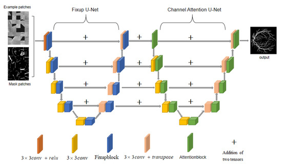
Figure 1. Structure of FAU-net.

The first de-normalized network uses an improved de-normalized residual block structure, which we call Fixupblock (Figure 2 right). Since it does not use batch normalization, the efficiency of the model is significantly improved. The second channel attention network adds the SCA module to Basicblock (Figure 3), called Attentionblock. We first input the patches of the original picture and the mask picture into the de-normalized network, which can quickly extract rough features of the blood vessel and send the feature values to the second channel attention network (Hereafter called CAU-Net). CAU-Net can model the interdependence between feature channels so that the weight of useful feature maps in the channel is higher than useless ones, and the weight of invalid or less useful feature maps is smaller so that features can be refined. The last layer of CAU-Net is the SoftMax layer, so the loss function we adopt is the negative log-likelihood loss function NLLLoss. Comparison experiments on three data sets with multiple state-of-the-art networks prove that our network has achieved the highest AUC value currently.

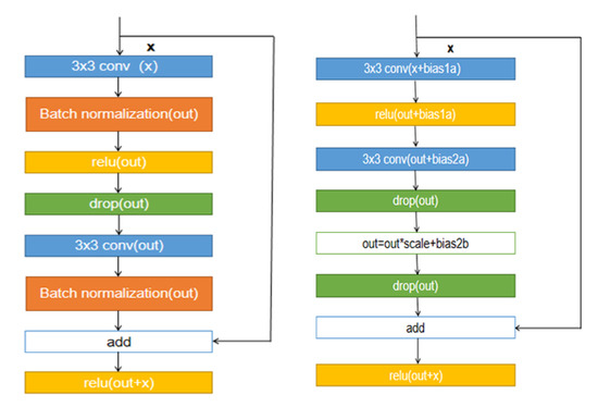
Figure 2. Resnet’s Basiclock structure on the left, and an improved Fixupblock structure on the right.

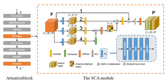
Figure 3. Left is the overall structure of the Attentionblock, right is the structure of the channel attention module SCA.

3.2. Improved De-Normalized Residuals Block

ResNet [27] was proposed in 2015, and its basic block is called the residual block. Residual block there are generally two kinds of forms, BasicBlock and Bottleneck, respectively. BasicBlock structure mainly uses two convolution sums of $3\times 3$. The branch of residual is:

$$\mathrm{OUT}=\mathrm{CONV}3\times 3+BN+RELU+\mathrm{CONV}3\times 3+BN$$

(1)

Then add it to the identity map and go through a RELU layer:

$$\mathrm{OUT}=\mathrm{OUT}+\mathrm{x}+\mathrm{RELU}$$

(2)

The structure of BasicBlock is shown on the left in Figure 2. The reason BasicBlock can work has a significant relationship with the BN layer it adds. Many residual networks cannot correctly account for the effects of residual connections without normalization techniques such as BatchNorm, resulting in gradient explosions. Lim et al. [28] experimentally verified that normalizing features using BN would eliminate the range flexibility of the network. Moreover, in the segmentation task of blood vessels, in order to obtain higher experimental accuracy, we often use larger batch size, which will significantly increase the memory usage of the GPU. A new initialization method [29] that does not require any normalization method was proposed. Based on this method, we propose an improved de-normalization block called Fixupblock. It appropriately adjusts the initial offset parameter at the beginning of training to ensure that the update of the network function (Gradient) stays in the proper range. It is independent of the network depth so that it can solve the problem of gradient explosion and gradient disappearance. At the same time, we add the two drop-out layers in Fixupblock to prevent some features from overfitting. It makes the weight update is no longer dependent on the combination of a stable relationship between hidden nodes. It avoids situations where certain features only work for certain other features, forcing the network to learn more robust features.

Improved Fixupblock structure shown in the right of Figure 2, where the bias term bias1a, bias2a, bias2a, bias2b all initialized to zero, the scale is initialized to one.

3.3. Channel Attention Module

Similar attention networks used for segmentation, such as [25,30], have bigger regions of interest and are more suitable for pathological segmentation. Our channel attention network can allocate the weight after each convolution and enhance the useful features, which is suitable for the segmentation of small blood vessels.

Generally, the output of the convolutional layer does not consider the channel dependence. We adopt the structure in SEblock [19], which is called Se calculation. It can enhance the effective features and suppress ineffective features between channels. We combine it with the channel attention module and propose a new channel attention module called SCA (Figure 3). Then add the SCA module to the second residual block of u-net and call it an Attentionblock (Figure 3). The following is the detailed calculation process of the channel attention module.

We assume that the original feature is $\mathrm{F}\in R^{\mathrm{C}\times \mathrm{H}\times \mathrm{W}}$, and the original feature goes through three pipelines 2, 3, and 4 as shown in Figure 3. After passing through these three pipelines, the original feature first undergoes Squeeze-and-Excitation calculation (Hereinafter referred to as Se).

In Se calculation, the first step is the Squeeze operation ${\mathrm{F}}_{sq}$, which is the operation of global average pooling:

$$Z_c=F_{sq}\left(f_c\right)=\frac{1}{H\times W}\sum _{i=1}^H\sum _{j=1}^W{f}_c(i,j)$$

(3)

Among them, $f_c$ represents the initial feature (i.e., the three-dimensional matrix $\mathrm{F}\in R^{\mathrm{C}\times \mathrm{H}\times \mathrm{W}}$), and the subscript c represents the c-th two-dimensional matrix in F, i.e., the channel. Equation (3) converts the input of $\mathrm{C}\times \mathrm{H}\times \mathrm{W}$ into $1\times 1\times C$, which indicates the numerical distribution of the c feature maps of the layer, i.e., the global information. The Squeeze operation in Equation (3) operated in the feature map of a channel, and the operation in Equation (4) is to fuse the weight of the feature map of each channel, i.e., the Excitation operation $F_{ex}$:

$$s=F_{ex}(z,W)=\sigma \left(g(z,W)\right)=\sigma \left(W_2\delta \left(W_{1}z\right)\right)$$

(4)

where z is the result of Equation (3), ${\mathrm{W}}_1$ multiplied by z is the first fully connected layer operation, and the dimension of ${\mathrm{W}}_1$ is $\frac{C}{r}\times \mathrm{C}$, where r is a scaling parameter, to reduce the number of channels and thus reduce the amount of calculation. In this paper, r sets to 2. The dimension of z is $1\times 1\times \mathrm{C}$, then the dimension of ${\mathrm{W}}_{1}z$ is $1\times 1\times \frac{C}{r}$. Then it goes through a RELU layer with the same dimensions, multiply it with ${\mathrm{W}}_2$, which is the operation of the second fully connected layer. The dimension of ${\mathrm{W}}_2$ is $c\times \frac{c}{r}$, and the dimension of output is $1\times 1\times \mathrm{C}$. Finally, the dimension is unchanged after passing the sigmoid function. The obtained s (Equation (4)) is the feature map weight of the channel learned through the previous fully connected and non-linear layers. It is the result of pipeline 2, 3, 4 after Se operation.

In pipeline 4, we transform the initial characteristics $\mathrm{F}\in R^{C\times \mathrm{H}\times \mathrm{W}}$ to $\mathrm{F}\in R^{C\times N}$, where $\mathrm{N}=\mathrm{H}\times W$ represents the pixels of the picture. Pipeline 3 was reshaped after SE processed the original features. Then perform matrix multiplication on the reshaped F and the transpose of F passing through pipeline 4, and finally use a SoftMax layer to get the channel attention map $\mathrm{X}\in {\mathrm{R}}^{\alpha }$:

$$x_{ij}=softmax(F_i·F_j)=\frac{exp(F_i·F_j)}{{\sum }_{i=1}^{C}exp(F_i·F_j)}$$

(5)

where $x_{ij}$ represents the influence of the i-th channel on the j-th channel.

In addition to the above operation, we perform matrix multiplication on the transpose of X and F obtained through pipeline 2 and reshape the result to ${\mathrm{R}}^{\mathrm{C}\times \mathrm{H}\times \mathrm{W}}$. Then multiply this result by a scale parameter $\beta$ and perform a pixel-level addition with F of pipeline 1 to get $\mathrm{E}\in {\mathrm{R}}^{\mathrm{C}\times \mathrm{H}\times \mathrm{W}}$:

$${\mathrm{E}}_{\mathrm{j}}=\beta \sum _{i=1}^{\mathrm{C}}\left(x_{ji}{F}_i\right)+F_j$$

(6)

Finally, the result E passes through a RELU and softmax layer, and the final feature is $\mathrm{P}\in R^{\mathrm{C}\times \mathrm{H}\times \mathrm{W}}$.

4. Quantitative Assessment Method

The segmentation of blood vessels is a binary classification problem. In classification problems, we usually use some indicators to evaluate the pros and cons of the algorithm. In this article, we use the values of Accuracy (AC), Precision, Recall, and Area under the ROC curve (AUC) and ${\mathrm{F}}_{\beta }-score$(${\mathrm{F}}_{\beta }$) evaluated the performance of FAU-net. We will use True Positive (TP), True Negative (TN), False Positive (FP), recall rate and False Negative (FN) to calculate the above indicators. Performance metrics calculation is as follows:

$$AC=\frac{TP+TN}{TP+TN+FP+FN}$$

(7)

$$Precision=\frac{TP}{TP+FP}$$

(8)

$$Recall=\frac{TP}{TP+FN}$$

(9)

We assume that the positive samples are pixels marked as blood vessels and the negative samples are background. We assign different weights to recall and precision to indicate the preference for classification models. The calculation equation is as follows:

$$F_{\beta }=\frac{\left(1+{\beta }^2\right)·Precision·Recall}{{\beta }^2·Precision+Recall}$$

(10)

It can be seen that when $\beta$ = 1, then ${\mathrm{F}}_{\beta }$ changes back to F1; when $\beta >1$, the model prefers to improve recall, which means that the model pays more attention to the ability to recognize positive samples. when $\beta <1$, the model pays more attention to the ability to distinguish negative samples. In this article, we do not want the model to produce the wrong results to cover more samples. It will affect the doctor’s diagnosis of the patient’s condition. Therefore, we will adjust the parameter $\beta$ to 0.75.

Considering the class imbalance of the data set, we also introduce Receiver Operating Characteristic (ROC) and Precision-Recall (PR) curves. The ROC curve is drawn with True Positive Rate (TPR) as the y-axis and False Positive Rate (FPR) as the x-axis. With the accuracy as the y-axis and the recall as the x-axis, we get the PR curve. The calculation equations of TPR and FPR are as follows:

$$TPR=\frac{TP}{TP+FN}$$

(11)

$$FPR=\frac{FP}{FP+TN}$$

(12)

5. Experiments

5.1. Training Parameters

Our network is an open-source framework based on Python 3.7, PyTorch 1.1.0. The experimental platform system is a Linux operating system (Ubuntu18.04), Intel Xeon E5-2620CPU@2.1 GHZ processor, 64 GB memory, Nvidia Titan Xp graphics card.

FAU-Net is trained for a total of 200 epochs. The learning efficiency set in the first 150 epochs is 0.001, and the learning efficiency of the last 50 epochs is 0.0001. This method of learning rate decay makes the model easier to approach the optimal solution. It consists of two 5-layer U-shaped networks, using Adam optimizer and cross-entropy loss function. In Fixupblock, we set initialization parameters bias term bias1a, bias2a, bias2a, bias2b all as 0, the scale as 1. The rate of the two drop-out layers is 0.25. We use a $3\times 3$ convolution with padding equals 1. In Attentionblock, the number of intermediate channels is 512, and the drop-out rate is 0.1.

5.2. Database Preparation

To evaluate the quality of the network, in addition to use the common retinal blood vessel dataset DRIVE, we also constructed two cerebral blood vessel datasets, called ELE and CORO datasets. For the selection of brain blood vessel data set, we mainly consider the problem of class imbalance. Our region of interest is blood vessels, so when selecting pictures, we should choose the more evenly distributed blood vessels. Otherwise, there will be many patches with only background but no blood vessels, which will reduce the accuracy of network training. The brain vascular data set is different from the retinal vascular data set in that it may have a more significant imbalance problem. The difficulty of retinal vascular segmentation is that there is no significant difference between the retinal vascular segmentation and the background. Compared with the data set of retinal vascular, ELE, and CORO brain blood vessel data set have a significant gap between the background and blood vessels, but there is a lot of noise. Moreover, the structure of the brain blood vessels is not coherent. It is easy to break during the segmentation, which can be a good evaluation of the performance of the segmentation network. How to make the overall structure of blood vessels clearer is the main problem we need to solve.

DRIVE data set [4]: We use the retinal vascular public data set DRIVE, and the brain blood vessel 3D CTA image data set ELE, and the brain blood vessel MRA data set. Each of their original images is 565 × 584 pixels in size.

ELE data set: The ELE data set consists of 40 colorful CTA images of the brain of different patients at different angles. Each image corresponds to an artificially labeled vascular mask picture, 20 pictures for training, and 20 samples for testing. The size of the image is 565 × 584 pixels.

CORO data set: The CORO data set consists of 40 brain MRA images, 20 pictures for training, and 20 samples for testing, which are images of multiple patients and multiple different angles. Each image corresponds to an artificially labeled vascular mask map, and the image size is 565 × 584 pixels.

Each picture in these three data sets will generate a square data set during training (see Figure 4). In order to improve the reliability of training results, 190,000 patches were randomly selected, among which $10\%$ was used as the verification data, of which 171,000 patches were used for training, and the remaining 19,000 patches were used for verification. The size of each patch was 48 × 48 pixels.

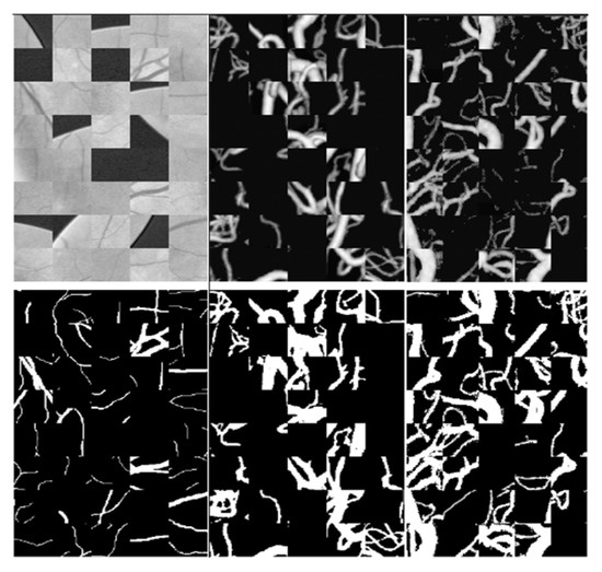
Figure 4. From left to right are the data sets DRIVE,ELE,CORO. Above are patches of the original image, and below are patches of the output results.

5.3. Segmentation Results and Discussion

Figure 5 shows the results of segmenting using FAU-Net. The first line is the grayscale image of the input image, the second line is the ground truth, and the third line is the experimental output. The first column is the result of the segmentation of the blood vessels of the eyeball. Compared with the marked pictures, our network can segment the marked vessels very well, even smaller vessels that are not marked.

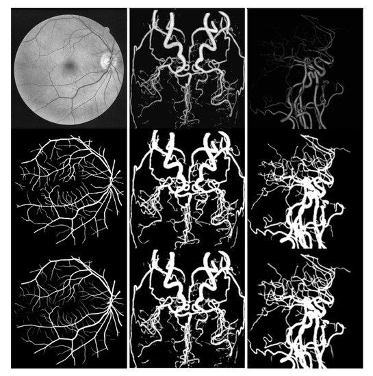
Figure 5. Complex vessel segmentation results. From left to right are the DRIVE, CORO, and ELE datasets.

The second column is the CORO segmentation result of the brain MRA vascular data set. From the segmentation results, we can distinguish between the blood vessel and the background noise, and there is less artifact information. Our segmentation makes the brain blood vessel the overall structure is clearer.

The third column is the segmentation result of our brain CTA image. The blood vessel structure of the CTA image is relatively simple, but it is difficult to distinguish the thinner and darker blood vessels from the image. Our network can distinguish these thinner and darker blood vessels well, enabling doctors to perform better medical analysis.

5.4. Comparative Experiments

We compare our network with the state-of-the-art models, such as U-Net, LadderNet, Dynamic Deep Networks, and IterNet, respectively, on three data sets, and use the standard evaluation method to evaluate.

Figure 6 shows the segmentation details of U-Net [3], LadderNet [16], Dynamic Deep Network [17], and our network on the three data sets of DRIVE, ELE, and CORO. See from a partially enlarged view of the image, our network can distinguish the retinal blood vessels from the background noise, and there is less noise in the boundary part of the eyeball. From the results of the segmentation of the ELE data set, our network can distinguish between thinner and darker one’s vascular structure. For the CORO data set, our segmentation made the vascular structure clearer and has fewer artifacts. Compared with other networks, the blood vessel structure segmented by our network is more complete and there are fewer broken blood vessels. In summary, we can say that our network has a more precise segmentation of small blood vessels than other networks, and has less background noise.

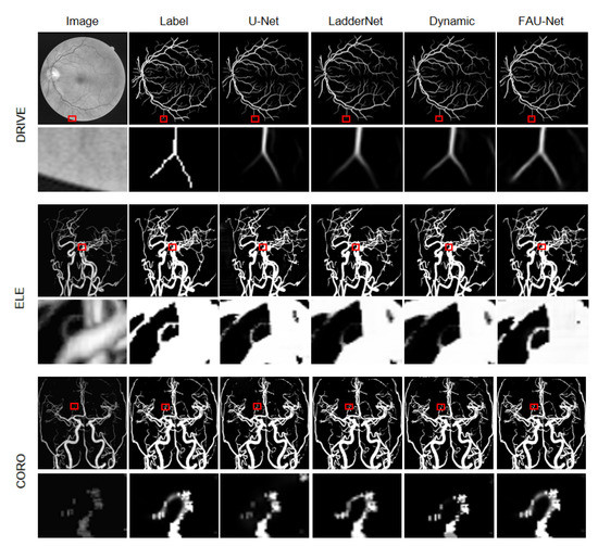
Figure 6. Visualization of the segmentation results on DRIVE, ELE, and CORO datasets.

Figure 7 shows the precision-recall curve and ROC curve obtained by running our network on the DRIVE data set. From the figure, we can see that the area under the precision-recall curve has reached 0.9100, and the area under the ROC curve reached 0.9853, indicating that our model is very robust. Figure 8 and Figure 9 show the precision-recall curve and ROC curve obtained by running our network on the ELE data set and the CORO data set, respectively, and their area under the curve has reached above 0.98.

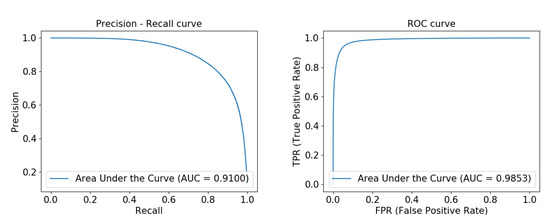
Figure 7. Precision-recall curve and ROC curve experimentally obtained from FAU-Net on the DRIVE data set from left to right.

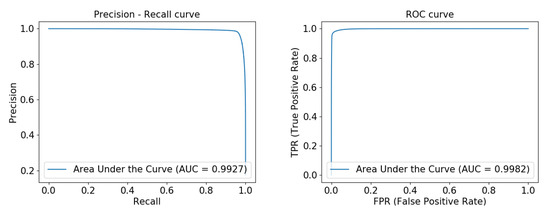
Figure 8. Precision-recall curve and ROC curve experimentally obtained from FAU-Net on the ELE data set from left to right.

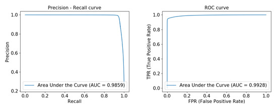
Figure 9. From left to right, the Precision-recall curve and ROC curve experimentally obtained on the CORO data set by FAU-Net.

We compared the three data sets to verify the effect of our improved de-normalization structure on vascular segmentation. The approach with fixup means that we replace the original Basicblock with Fixupblock and do not use the channel attention mechanism. The data with the bold font in the table is the better data result. The last digit is the result of rounding. All data are the result of training 200 epochs.

Table 1 compares the results of the original U-net, LadderNet, and U-net using the de-normalized structure on the DRIVE data set. AUC has improved. LadderNet, which uses a de-normalized structure, has achieved better results in both Precision and ${\mathrm{F}}_{\beta }$-score. Table 2 and Table 3 compare the test results of U-net and LadderNet on the ELE and CORO data sets, respectively. Under the de-normalized structure, U-net’s various indicators under the ELE data set have improved and achieved better performance. On the CORO data set, the results of using the de-normalized u-net and the original u-net are not large, and the original LadderNet achieves better performance on ${\mathrm{F}}_{\beta }$-score and AUC. According to the results of these experiments, better segmentation accuracy can be obtained using the improved de-normalization method.

Table 1. Results on DRIVE data set.

Methods	Accuracy	Precision	${\mathbf{F}}_{\mathit{\beta }}$-Score	AUC
U-net	0.9531	0.8852	0.8142	0.9755
U-net with fixup	0.9561	0.8612	0.8196	0.9783
LadderNet	0.9561	0.8593	0.8202	0.9793
LadderNet with fixup	0.9572	0.8616	0.8305	0.9779

Table 2. Results on ELE data set.

Methods	Accuracy	Precision	${\mathbf{F}}_{\mathit{\beta }}$-Score	AUC
U-net	0.9801	0.9631	0.9486	0.9875
U-net with fixup	0.9891	0.9735	0.9685	0.9982
LadderNet	0.9890	0.9709	0.9688	0.9983
LadderNet with fixup	0.9896	0.9717	0.9692	0.9982

Table 3. Results on CORO data set.

Methods	Accuracy	Precision	${\mathbf{F}}_{\mathit{\beta }}$-Score	AUC
U-net	0.9801	0.9784	0.9633	0.9808
U-net with fixup	0.9847	0.9914	0.9721	0.9960
LadderNet	0.9842	0.9906	0.9723	0.9962
LadderNet with fixup	0.9843	0.9918	0.9695	0.9957

Table 4 compares the experimental results of our network with the current state-of-the-art network for vascular image segmentation on three data sets. On two data sets, DRIVE and ELE, our network has made significant improvements to Accuracy, ${\mathrm{F}}_{\beta }$-score, and AUC. These indicators are more critical for vascular segmentation. On the CORO data set, our network also has significant improvements in the two indicators, Accuracy and AUC. The area under our network-trained ROC curve and the precision-recall curve has achieved Accuracy above 0.9 on all three data sets, which shows that our model is more efficient and robust.

Table 4. Experimental results of FAU-net compared with other networks on DRIVE, ELE, CORO data sets.

Dataset	Year	Methods	Accuracy	Precision	${\mathbf{F}}_{\mathit{\beta }}$-Score	AUC
DRIVE	2015	U-net [3]	0.9531	0.8852	0.8142	0.9755
	2018	Recurrent U-Net [15]	0.9556	0.8603	0.8155	0.9782
	2018	Residual U-Net [15]	0.9553	0.8614	0.8149	0.9779
	2018	R2U-Net [15]	0.9556	0.8589	0.8171	0.9784
	2018	LadderNet [16]	0.9561	0.8593	0.8202	0.9793
	2019	Dynamic Deep Networks [17]	0.9693	0.8284	0.8259	0.9775
	2020	IterNet(Patched) [18]	0.9573	0.8534	0.8205	0.9816
	2020	FAU-net	0.9698	0.8651	0.8320	0.9853
ELE	2015	U-net	0.9801	0.9631	0.9486	0.9875
	2018	Recurrent U-Net	0.9776	0.9736	0.9465	0.9930
	2018	Residual U-Net	0.9837	0.9670	0.9582	0.9902
	2018	R2U-Net	0.9806	0.9501	0.9684	0.9955
	2018	LadderNet	0.9889	0.9709	0.9685	0.9980
	2019	Dynamic Deep Networks	0.9816	0.9435	0.9684	0.9942
	2020	IterNet(Patched)	0.9821	0.9664	0.9568	0.9961
	2020	FAU-net	0.9891	0.9695	0.9688	0.9982
CORO	2015	U-net	0.9801	0.9784	0.9633	0.9808
	2018	Recurrent U-Net	0.9739	0.9806	0.9541	0.9912
	2018	Residual U-Net	0.9716	0.9792	0.9498	0.9755
	2018	R2U-Net	0.9786	0.9892	0.9642	0.9893
	2018	LadderNet	0.9843	0.9906	0.9723	0.9962
	2019	Dynamic Deep Networks	0.9798	0.9758	0.9649	0.9897
	2020	IterNet(Patched)	0.9739	0.9825	0.9654	0.9953
	2020	FAU-net	0.9834	0.9932	0.9730	0.9928

Table 5 shows the calculation time for the test phase of each sample. We compared the U-Net, Recurrent U-Net, Residual U-Net, LadderNet, Dynamic Deep Networks, IterNet(Patched), R2U-Net and FAU-Net on the three blood vessel data set DRIVE and the brain blood vessel data sets ELE and CORO, respectively. Results proved that our model could achieve high accuracy under high efficiency.

Table 5. Computational time for testing(Time (s)/sample).

Dataset	DRIVE	ELE	CORO
U-Net	2.16 s	2.35 s	2.05 s
Recurrent U-Net	5.23 s	4.56 s	4.23 s
Residual U-Net	3.57 s	4.16 s	3.13 s
R2U-Net	5.75 s	2.54 s	5.34 s
IterNet (Patched)	16.53 s	14.45 s	15.86 s
LadderNet	1.78 s	2.01 s	1.41 s
Dynamic Deep Networks	4.72 s	4.23 s	3.88 s
FAU-Net	1.43 s	1.27 s	1.21 s

Taking a comprehensive look at Table 1, Table 2 and Table 3 and Table 5, we can see that using this de-normalized structure not only can get good experimental results but also can significantly reduce the computational time for testing. It is significant for clinical applications.

6. Conclusions and Future Work

This paper proposes a de-normalized channel attention network based on a dual U-Net structure. De-normalized blocks and channel attention modules were added to accurately segment sophisticated blood vessels such as retinal blood vessels and brain blood vessels, and our experiments have achieved superior results. To test the impact of the de-normalized block on the segmentation network, we examined the effects using batch normalization and de-normalization on three data sets and compared them. Experiments show that our de-normalized block can improve network performance and robustness while achieving higher accuracy. In the next step, we will continue to refine our segmentation network and apply the segmentation results to the vascular navigation path planning.

References

- Japkowicz, N.; Stephen, S. The class imbalance problem: A systematic study. Intell. Data Anal. 2002, 6, 429–449. [Google Scholar] [CrossRef]
- Cubuk, E.D.; Zoph, B.; Mane, D.; Vasudevan, V.; Le, Q.V. Autoaugment: Learning augmentation policies from data. arXiv 2018, arXiv:1805.09501. [Google Scholar]
- Ronneberger, O.; Fischer, P.; Brox, T. U-net: Convolutional networks for biomedical image segmentation. In Proceedings of the International Conference on Medical Image Computing and Computer-Assisted Intervention, Munich, Germany, 5–9 October 2015; Springer: Berlin/Heidelberg, Germany, 2015; pp. 234–241. [Google Scholar]
- Staal, J.; Abramoff, M.; Niemeijer, M.; Viergever, M.A.; Van Ginneken, B. Ridge-based vessel segmentation in color images of the retina. IEEE Trans. Med. Imaging 2004, 23, 501–509. [Google Scholar] [CrossRef] [PubMed]
- Al-Amri, S.S.; Kalyankar, N.V. Image segmentation by using threshold techniques. arXiv 2010, arXiv:1005.4020. [Google Scholar]
- Gould, S.; Gao, T.; Koller, D. Region-based segmentation and object detection. In Proceedings of the Advances in Neural Information Processing Systems, Vancouver, BC, Canada, 7–10 December 2009; pp. 655–663. [Google Scholar]
- Sumengen, B.; Manjunath, B. Multi-scale edge detection and image segmentation. In Proceedings of the 2005 13th IEEE European Signal Processing Conference, Antalya, Turkey, 4–8 September 2005; pp. 1–4. [Google Scholar]
- Zhang, G.M.; Chen, S.P.; Liao, J.N. Otsu image segmentation algorithm based on morphology and wavelet transformation. In Proceedings of the 2011 3rd IEEE International Conference on Computer Research and Development, Shanghai, China, 11–13 March 2011; Volume 1, pp. 279–283. [Google Scholar]
- Maulik, U. Medical image segmentation using genetic algorithms. IEEE Trans. Inf. Technol. Biomed. 2009, 13, 166–173. [Google Scholar] [CrossRef] [PubMed]
- Fan, Y.; Jiang, T.; Evans, D.J. Volumetric segmentation of brain images using parallel genetic algorithms. IEEE Trans. Med. Imaging 2002, 21, 904–909. [Google Scholar] [PubMed]
- Wang, L.; Li, C.; Sun, Q.; Xia, D.; Kao, C.Y. Active contours driven by local and global intensity fitting energy with application to brain MR image segmentation. Comput. Med. Imaging Graph. 2009, 33, 520–531. [Google Scholar] [CrossRef] [PubMed]
- Long, J.; Shelhamer, E.; Darrell, T. Fully convolutional networks for semantic segmentation. In Proceedings of the IEEE Conference on Computer Vision and Pattern Recognition, Boston, MA, USA, 7–12 June 2015; pp. 3431–3440. [Google Scholar]
- Korez, R.; Likar, B.; Pernuš, F.; Vrtovec, T. Model-based segmentation of vertebral bodies from MR images with 3D CNNs. In Proceedings of the International Conference on Medical Image Computing and Computer-Assisted Intervention, Athens, Greece, 17–21 October 2016; Springer: Berlin/Heidelberg, Germany, 2016; pp. 433–441. [Google Scholar]
- Zhou, X.; Ito, T.; Takayama, R.; Wang, S.; Hara, T.; Fujita, H. Three-dimensional CT image segmentation by combining 2D fully convolutional network with 3D majority voting. In Deep Learning and Data Labeling for Medical Applications; Springer: Berlin/Heidelberg, Germany, 2016; pp. 111–120. [Google Scholar]
- Alom, M.Z.; Hasan, M.; Yakopcic, C.; Taha, T.M.; Asari, V.K. Recurrent residual convolutional neural network based on u-net (R2U-net) for medical image segmentation. arXiv 2018, arXiv:1802.06955. [Google Scholar]
- Zhuang, J. LadderNet: Multi-path networks based on U-Net for medical image segmentation. arXiv 2018, arXiv:1810.07810. [Google Scholar]
- Khanal, A.; Estrada, R. Dynamic Deep Networks for Retinal Vessel Segmentation. arXiv 2019, arXiv:1903.07803. [Google Scholar] [CrossRef]
- Li, L.; Verma, M.; Nakashima, Y.; Nagahara, H.; Kawasaki, R. IterNet: Retinal Image Segmentation Utilizing Structural Redundancy in Vessel Networks. In Proceedings of the IEEE Winter Conference on Applications of Computer Vision (WACV), Snowmass Village, CO, USA, 1–5 March 2020. [Google Scholar]
- Hu, J.; Shen, L.; Sun, G. Squeeze-and-excitation networks. In Proceedings of the IEEE Conference on Computer Vision and Pattern Recognition, Salt Lake City, UT, USA, 18–22 June 2018; pp. 7132–7141. [Google Scholar]
- Zhang, H.; Dana, K.; Shi, J.; Zhang, Z.; Wang, X.; Tyagi, A.; Agrawal, A. Context encoding for semantic segmentation. In Proceedings of the IEEE Conference on Computer Vision and Pattern Recognition, Salt Lake City, UT, USA, 18–22 June 2018; pp. 7151–7160. [Google Scholar]
- Li, H.; Xiong, P.; An, J.; Wang, L. Pyramid attention network for semantic segmentation. arXiv 2018, arXiv:1805.10180. [Google Scholar]
- Fu, J.; Liu, J.; Tian, H.; Li, Y.; Bao, Y.; Fang, Z.; Lu, H. Dual attention network for scene segmentation. In Proceedings of the IEEE Conference on Computer Vision and Pattern Recognition, Long Beach, CA, USA, 16–20 June 2019; pp. 3146–3154. [Google Scholar]
- Oktay, O.; Schlemper, J.; Folgoc, L.L.; Lee, M.; Heinrich, M.; Misawa, K.; Mori, K.; McDonagh, S.; Hammerla, N.Y.; Kainz, B.; et al. Attention u-net: Learning where to look for the pancreas. arXiv 2018, arXiv:1804.03999. [Google Scholar]
- Sinha, A.; Dolz, J. Multi-scale guided attention for medical image segmentation. arXiv 2019, arXiv:1906.02849. [Google Scholar] [CrossRef] [PubMed]
- Bastidas, A.A.; Tang, H. Channel Attention Networks. In Proceedings of the 2019 IEEE/CVF Conference on Computer Vision and Pattern Recognition Workshops (CVPRW), Long Beach, CA, USA, 16–20 June 2019; pp. 881–888. [Google Scholar]
- Ghani, A.; See, C.; Sudhakaran, V.; Ahmad, J.; Abd-Alhameed, R. Accelerating retinal fundus image classification using artificial neural networks (ANNs) and reconfigurable hardware (FPGA). Electronics 2019, 8, 1522. [Google Scholar] [CrossRef]
- He, K.; Zhang, X.; Ren, S.; Sun, J. Deep residual learning for image recognition. In Proceedings of the IEEE Conference on Computer Vision and Pattern Recognition, Las Vegas, NV, USA, 27–30 June 2016; pp. 770–778. [Google Scholar]
- Lim, B.; Son, S.; Kim, H.; Nah, S.; Mu Lee, K. Enhanced deep residual networks for single image super-resolution. In Proceedings of the IEEE Conference on Computer Vision and Pattern Recognition Workshops, Honolulu, HI, USA, 21–26 July 2017; pp. 136–144. [Google Scholar]
- Zhang, H.; Dauphin, Y.N.; Ma, T. Fixup initialization: Residual learning without normalization. arXiv 2019, arXiv:1901.09321. [Google Scholar]
- Wang, F.; Jiang, M.; Qian, C.; Yang, S.; Li, C.; Zhang, H.; Wang, X.; Tang, X. Residual Attention Network for Image Classification. In Proceedings of the 2017 IEEE Conference on Computer Vision and Pattern Recognition (CVPR), Honolulu, HI, USA, 21–26 July 2017; pp. 6450–6458. [Google Scholar]
© 2020 by the authors. Licensee MDPI, Basel, Switzerland. This article is an open access article distributed under the terms and conditions of the Creative Commons Attribution (CC BY) license (http://creativecommons.org/licenses/by/4.0/).