Article

Development and Research of a Multi-Medium Motion Capture System for Underwater Intelligent Agents

1
College of Electronics and Information Engineering, Tongji University, Shanghai 201804, China
2
Data Science Institute, Columbia University, New York, NY 10027, USA
*
Author to whom correspondence should be addressed.
These authors contributed equally to this work.
Appl. Sci. 2020, 10(18), 6237; https://doi.org/10.3390/app10186237
Submission received: 17 August 2020 / Revised: 30 August 2020 / Accepted: 3 September 2020 / Published: 8 September 2020
(This article belongs to the Special Issue Underwater Image)

Abstract

:

Featured Application

A potential application of the work is research and design of autonomous underwater vehicle, especially the development of bionicfish-robots.

Abstract

A multi-medium motion capture system based on markers’ visual detection is developed and experimentally demonstrated for monitoring underwater intelligent agents such as fish biology and bionic robot-fish. Considering the refraction effect between air and water, a three-dimensional (3D) reconstruction model is established, which can be utilized to reconstruct the 3D coordinate of markers underwater from 2D data. Furthermore, the process of markers matching is undertaken through the multi-lens fusion perception prediction combined K-Means clustering algorithm. Subsequently, in order to track the marker of being occluded, according to the kinematics information of fish, an improved Kalman filtering algorithm is proposed. Finally, the feasibility and effectiveness of proposed system are verified through experimental results. The main models and methods in this paper can provide a reference and inspiration for measurement of underwater intelligent agents.

1. Introduction

As a new kind of autonomous underwater vehicle (AUV) combined with propulsion mechanism of fish and robotics, the bionic robot-fish has been widely applied in water quality monitoring, scientific underwater exploration, oceanic supervision and fishery conservation [1,2,3,4], because of several advantages, compared with traditional AUV based on screw propeller, such as low energy consumption, low noise, high propulsion efficiency and high mobility [5]. Nevertheless, the bionic robot-fish still has a large gap in speed, propulsive efficiency and maneuverability in comparison with biological prototype. Therefore, in order to improve the swimming performance of robotic fish, exploring the locomotion patterns of fish through movement observation are the essential issues. Among the available techniques used in observation of fish swimming [6,7,8,9], the vision-based method is considered to be a simple, low cost and easily available one for high precision [10], and has attracted extensive attention from researchers. Budick used a high-speed camera (500 fps) to photograph the swimming and turning behavior of juvenile zebra fish to study the effects of nervous system on fish swimming [11]. Bartol used the Kodak high-speed camera (500~1000 fps) to shoot the movement of squid in the shallow water and obtained its swimming strategy at different speed [12]. For obtaining the actual fish locomotion data, Yan measured the fish swimming modes by camera set up in the upper area of the water tank and five colored markers attached to the fish body from tail to head, and the motion data will be derived from the five markers data [13]. In this system, the marker should contrast sharply with the fish in gray scale. Consequently, Lai proposed a marker less observation method to measure the fish locomotion [14]. However, in the above studies, the information of only one or two planes are concerned, some kinematics data are ignored and accurate three-dimensional information cannot be obtained. To get the three-dimensional (3D) coordinates of fish in the tank, Pereira proposed a method that combines a single camera with a waterproof mirror, in which a waterproof mirror is placed at the angle of 45° on the side of tank for achieving the equivalent of another camera shooting horizontally [15], but because the image captured by the virtual camera is the inverted image, the reconstruction error is large. Viscido recorded the fish swimming information in the XY and XZ coordinate surface by two cameras set up, respectively, above vertically and in front of the tank [16], while it still has error when the fish swimming near the front wall of tank. Besides, Zhu obtained the 3D information by using a camera and two plane mirrors according to the plane mirror imaging principle [17], which is similar to the [15]. Oya reconstructed the 3D information from 2D images captured by two cameras based on the principle of triangulation [18]. These studies show that vision-based approaches can be easy to design and quick to implement for reconstructing the 3D motion data of fish. However, due to the light refraction that occurs at water-air interface, the reconstruction accuracy is greatly reduced and there is no investigation has been conducted that considers the light refraction for capturing the fish motion.
The distortion in 3D reconstruction caused by the refraction should be solved in order to perform more accurate 3D reconstruction. A recent literature review show that the researchers along with the hardware supports allows developing algorithms to do high processing calculation for 3D reconstruction task in many fields [19]. A refractive estimator derived by Anne et al. for sparse two-view geometry show that the proposed refractive method outperforms the perspective method in a controlled lab environment for deep sea applications [20]. A skeleton-based multiple fish 3-D tracking method is proposed in [21], and machine learning will be adopted for improving the tracking performance in their future work. Ichimaru created a real underwater stereo database by developing a special bubble generation device and put forward a CNN-based target-region extraction method for 3D shape acquisition of live fish and swimming humans. Ichimaru suggests that the reconstructed depth discretization should be further addressed in the future [22]. The above literature shows that 3D reconstruction technology based on underwater images has good application prospects, but it still needs to be studied and improved.
In this paper, we develop a multi-markers-based motion capture system of fish considering the refraction effect, where eight cameras are set up to simultaneously shoot the markers from different angles for reconstructing the 3D space information of fish movement. Firstly, according to the characteristics of light refraction, the multi-medium 3D reconstruction algorithm based on the least square method is proposed. Meanwhile, aiming at the markers matching problem, the markers are filtered with the constrains of fish speed and others, then the markers matching is realized by K-Means clustering algorithm. In addition, an adaptive Kalman filter model with overall movement information of fish is put forward to solve the marker occlusion. Then the error and the correction method of underwater 3D reconstruction is analyzed. Finally, the motion capture experiment of live fish is established, and a corresponding software system is designed for on-line and real-time monitoring. The paper is organized as follows. The Section 2 presents the multi-medium 3D reconstruction model. In Section 3 and Section 4, the markers matching method based on the images by different cameras and marker tracking algorithm are presented. In Section 5, the reconstruction error is analyzed, and in Section 6, the live fish experiments are given to verify the effectiveness of proposed system. Finally, Section 7 gives the conclusion and discussion.

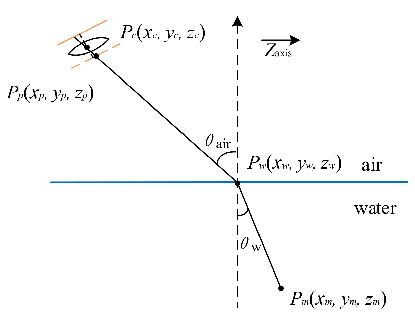
2. Three-Dimensional Reconstruction Model
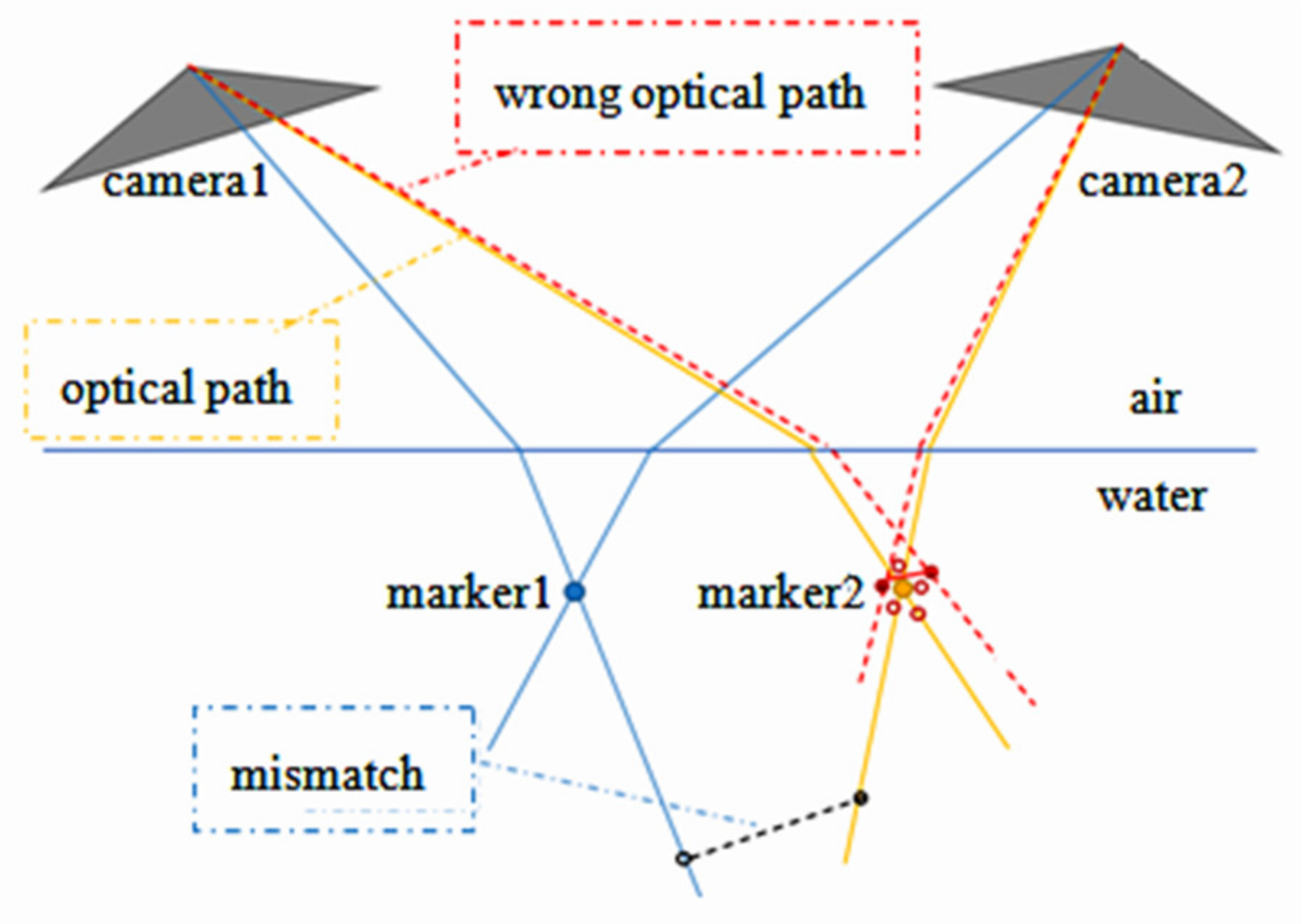
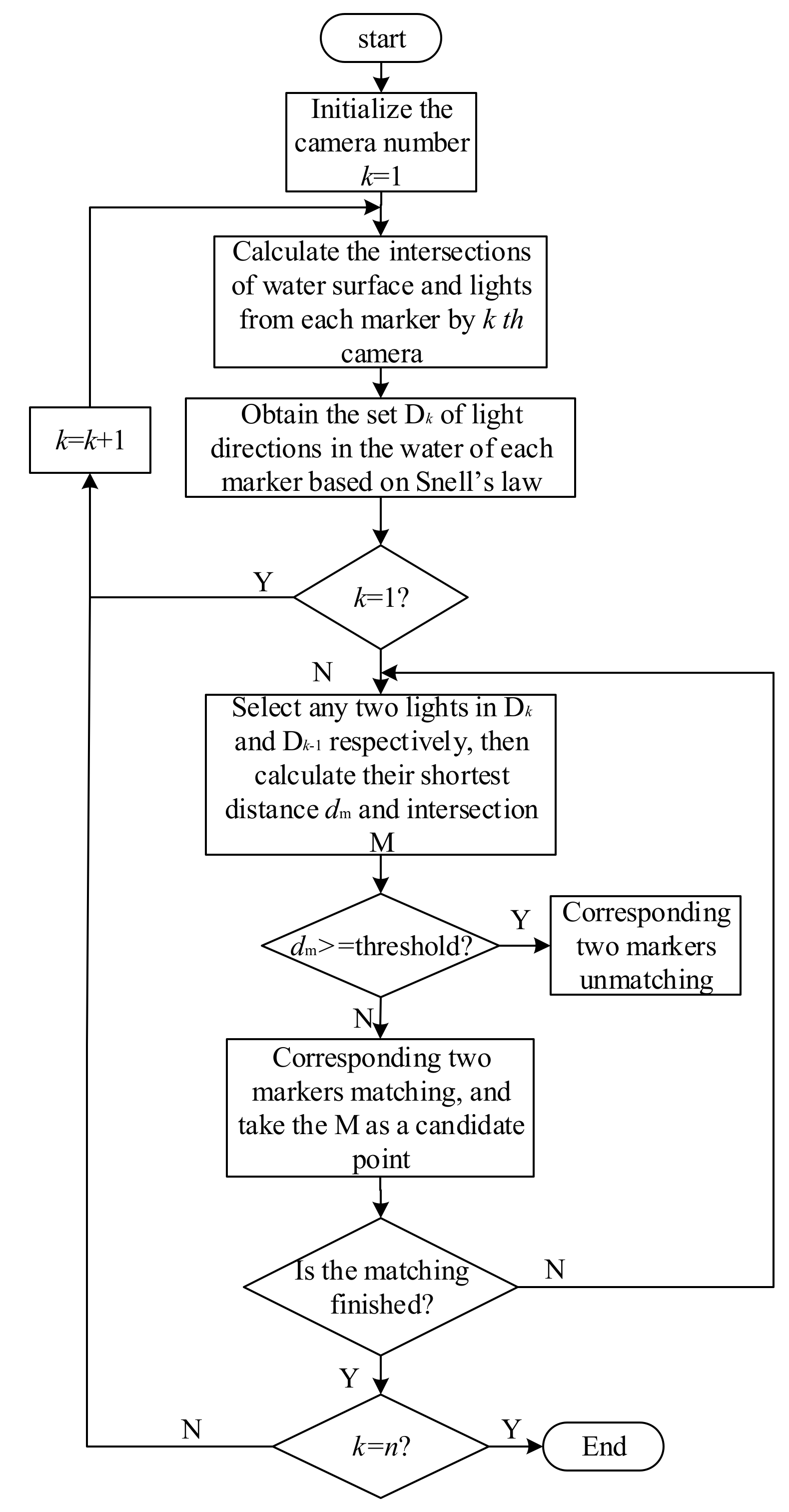
In order to study the effect of refraction on 3D reconstruction of markers, the process of light beam emitted from the marker to the camera is considered: the light emitted from marker reaches the water surface and be bent due to the different refractive index of water and air, then reaches the camera imaging plane through camera lens. The refraction process follows Snell’s law:
n a i r sin θ a i r = n w a t e r sin θ w a t e r
where n a i r and n w a t e r are the refractive indices of air and water respectively, θ a i r and θ w a t e r represents the angles of incidence and refraction respectively.
The fish swims generally at the bottom of tank, which means the fluctuations in the water surface are small and can be ignored. Therefore, the model can be simplified into a refraction model that is shown in Figure 1.
Where the P c is the position of the camera light spot, P m is the actual position of the marker point, and P w and P p are, respectively, the intersections of light and water and imaging plane.
Calibrated by camera, the P c x c , y c , z c is known. The P p x p , y p , z p can be obtained by using Equation (2) based on its 2D coordinates u p , v p on the imaging plane and the camera parameters.
x p y p z p 1 = R 3 * 3 t 3 * 1 0 1 1 K 1 α u p v p 1
where the R 3 × 3 and t 3 × 1 are, respectively, orthogonal rotation matrix and translation matrix, all of which are the external parameters of camera. The K and α are the intrinsic parameters of camera.
Meanwhile, the height of water surface is known and P w is on the extension line of P c P p , according to Snell’s law and the following equations
sin θ air = P w P c × Z a x i s P w P c Z a x i s
sin θ water = P w P m × Z a x i s P w P m Z a x i s
We can obtain
1 γ x w x m 2 + y w y m 2 = γ z w z m 2
where
γ = n air n water 2 x w x c 2 + y w y c 2 x w x c 2 + y w y c 2 + Z w Z c 2
Because the focal points of P c , P w , P m and P p projected on water surface are coplanar, the Equation (7) is satisfied.
0 0 z c x m x w y m y w z m z w x w x c y w y c z w z c = 0
That is
x m x w y w y c = x w x c y m y w
Combining the Equations (5) and (8), and assuming that the horizontal plane is above the object, that is z w z m 0 , the equations of unknown parameters of x m , y m and z m can be expressed as a matrix and shown in Equation (9).
1 0 λ 1 γ λ 2 + 1 0 γ x w + λ y w 1 γ λ 2 + 1 y w + γ z w x m y m z m 1 = 0 y m y w 1 0 λ 1 γ λ 2 + 1 0 γ x w + λ y w 1 γ λ 2 + 1 y w + γ z w x m y m z m 1 = 0 y m > y w
where
λ = x w x c y w y c
In general, the 3D reconstruction of a marker requires it to be captured by at least two cameras; therefore, the position of marker P m can be obtained by solving n simultaneous Equation (9) (n is the number of cameras which have captured the markers).

3. Markers Matching

Because of the light source, scattering and other issues, the markers captured by camera and displayed on screen have a certain deviation in color. Therefore, a larger number of marker colors is not better. With these considerations, three very different colors: red, green and blue, are selected for markers. Nevertheless, it will introduce another issue that there exist more than one of the same colored markers in corresponding frames by different cameras.
In this section, we firstly simplify markers matching process in the first frame body according to body structure of fish, and based on that, propose the matching method with forecast in subsequent frames, then classify the markers that have been matched through K-means clustering algorithm. Finally, the markers matching is accomplished.

3.1. First Frame

Take the case of two cameras, for example, because of the error, the two lights from same marker cannot be intersected in the water. As shown in Figure 2, the yellow line indicates the light in the ideal case and the red line indicates the light in actual measurement, hence the intersection point cannot be used to judge whether markers are matched. Despite the two lights being in different planes, their vertical distance is short, especially compared to the shortest distance of the optical path of unmatched markers. Hence, the shortest distance of the light can be used as the basis to filter the data. If the shortest distance of light is greater than the threshold, the markers must be unmatched. Because the general marker will be captured by more than two cameras, we can get many measurement points near the actual position of the marker. If there is more than a pair of measurement points in the vicinity, they must be matched.
Due to the flat structure of fish, the markers are set on both sides of fish body and the cameras which have captured same marker are adjacent. To simplify the calculation, the candidate points of 3D reconstruction can be obtained by consecutively matching two adjacent cameras.
The markers matching process is shown in Figure 3. Assume that the intrinsic parameters and pose of each camera and 2D coordinates of each marker on the image are known. The flow chart demonstrates how the markers, originally in 2D coordinates, become the candidate points through the coordinate system conversion and data screening.

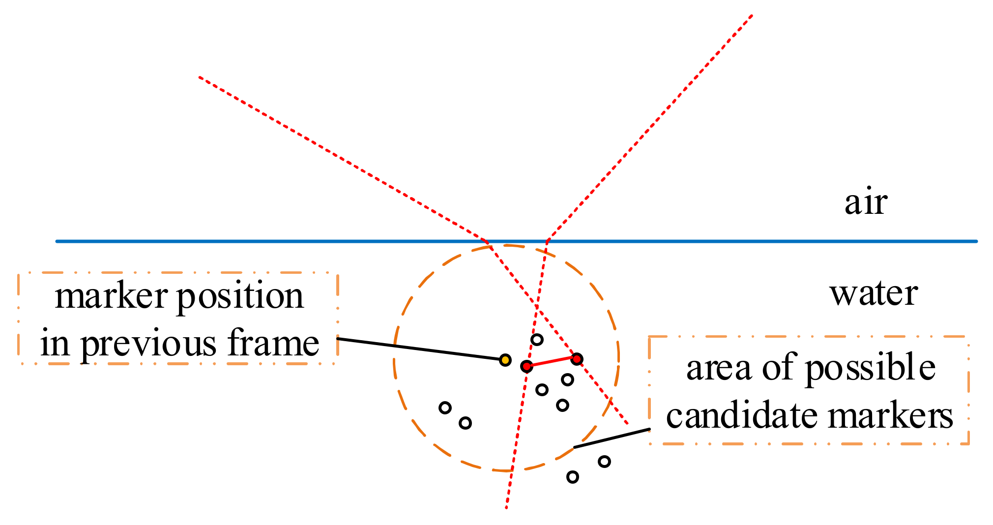
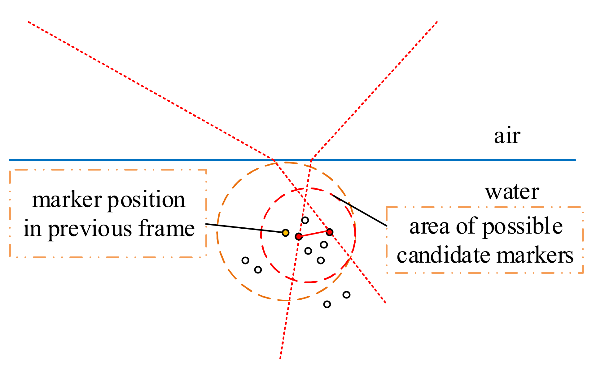
3.2. In Subsequent Frames

In general, the swim speed of the freshwater fish is within 120 cm/s, and the frame rate of the GoPro camera that we used in the experiment is 120 fps, which results in the moving range of the marker between adjacent frames being within 10 mm. Therefore, it can be regarded that the marker in the current frame is confined in a spherical area, the center of which is the marker in the previous frame, with a radius of 10 mm, as shown in Figure 4.
Due to various factors such as speed, comparing with previous frame, the points in the current frame are not evenly distributed in the spherical area. We use Kalman Filtering, because of the speed, acceleration and other factors, to narrow the candidate area. This is shown in Figure 5.

3.3. Markers Classification

When the total number of markers is known, the K-means algorithm can be utilized to classify the candidate points, and then the spatial positions of the markers are finally obtained by Equation (9).
According to the characteristics of the data in this paper, we can select K candidate points as the K-means initial clustering center, and then calculate the distance between all candidate markers and K centers. If the candidate marker P i   is closest to the clustering center C j , P i   belongs to the C j   cluster. Then recalculate C j , the new position of C j is the arithmetic mean of all the marker points belonging to this cluster. Next, recalculate C j , the new position is the arithmetic mean of all markers belonging to the cluster. Then update the candidate markers that are contained in each cluster again until the cluster is no longer changed. Because there may be a wrong point in the data we use, that is, non-matching points are also clustered in candidate points, we need to filter the points within the cluster. Calculate the distance between each point in the cluster and its cluster center. If all distances are less than 10 mm, then the cluster is considered to be unmistakable. If not, we consider that a wrong point exists. Then, remove the point which has farthest distance away from the center and recalculate the center position, repeat the method above until all distances between points and its cluster center are less than 10 mm.
It should be noted that, for the subsequent frames, taking the marker position of previous frame as the initial clustering center can improve the clustering accuracy and speed.

4. Marker Tracking

In the motion capture system, there will be a problem that the marker cannot be reconstructed because it is occluded or only captured by one camera, and at present, in most motion capture systems, it can be solved by employing the differential simulation method based on human body model where the adjacent joints are considered as rigid connections. However, the above method is not suitable for fish because the fish spine cannot be simulated with a rigid connection. According to the kinematic characteristics of fish, the body undulation model is related to the time and its motion period is unmeasurable in a short time. Therefore, we adopt the mean-variance adaptive Kalman filter to track the marker being occluded. Additionally, considering the movements of markers stuck to the fish body are consistent, the overall movement information is added to the filter link to improve the prediction effect.

4.1. Mean-Variance Adaptive Kalman Filter

In this paper, the system state vector includes the position, velocity and acceleration of the marker and is represented as
X t = x t x ˙ t x ¨ t
The state equation can be expressed by
x ˙ t x ¨ t x t = 0 1 0 0 0 1 0 0 α x t x ˙ t x ¨ t + 0 0 α a ¯ + 0 0 1 ω t
where the a ¯ is the mean value of acceleration.
Assuming the sampling period is T, after discretization, the state equations at the time of t k is
X k = Φ X k 1 + a ¯ U + W k
where the W k is the perturbing noise, which is white noise with normal distribution, the Φ and U are the state transition matrix and control vector respectively, which are shown as follows.
Φ = 1 T 1 α 2 1 + α T + e α T 0 1 1 α 1 e α T 0 0 e α T
U = 1 α T + α T 2 2 + 1 e α T α T 1 e α T α 1 e α T
The observation equation is
Z k = H X k + V k
where H is the transfer matrix that represents the transformation relation between vectors of state and observation, V k is the observation noise.
Hence, the prediction equations of state and covariance are shown as
X ^ k | k 1 = Φ X ^ k 1 | k 1 + a ¯ U
P k | k 1 = Φ P k 1 | k 1 Φ T + Q k
where the a ¯ is taken as a step of acceleration prediction.
The equations of filter gain, state update and covariance update are summarized as follows:
K k = P k | k 1 H T H P k | k 1 H T + R k 1
X ^ k | k = X ^ k | k 1 + K k Z k H X ^ k | k 1
P k | k = P k | k 1 K k H P k | k 1
where the R k stands for the covariance matrix of observation noise.

4.2. Marker Tracking with Improved Kalman Filter

In order to improve the tracking precision, in this section, the kinematic model of fish is considered in the process of marker tracking and the improved adaptive Kalman Filter is proposed.

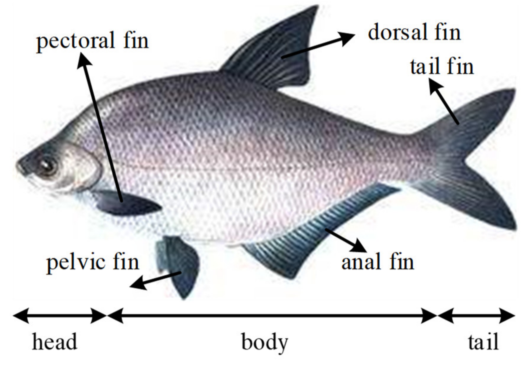
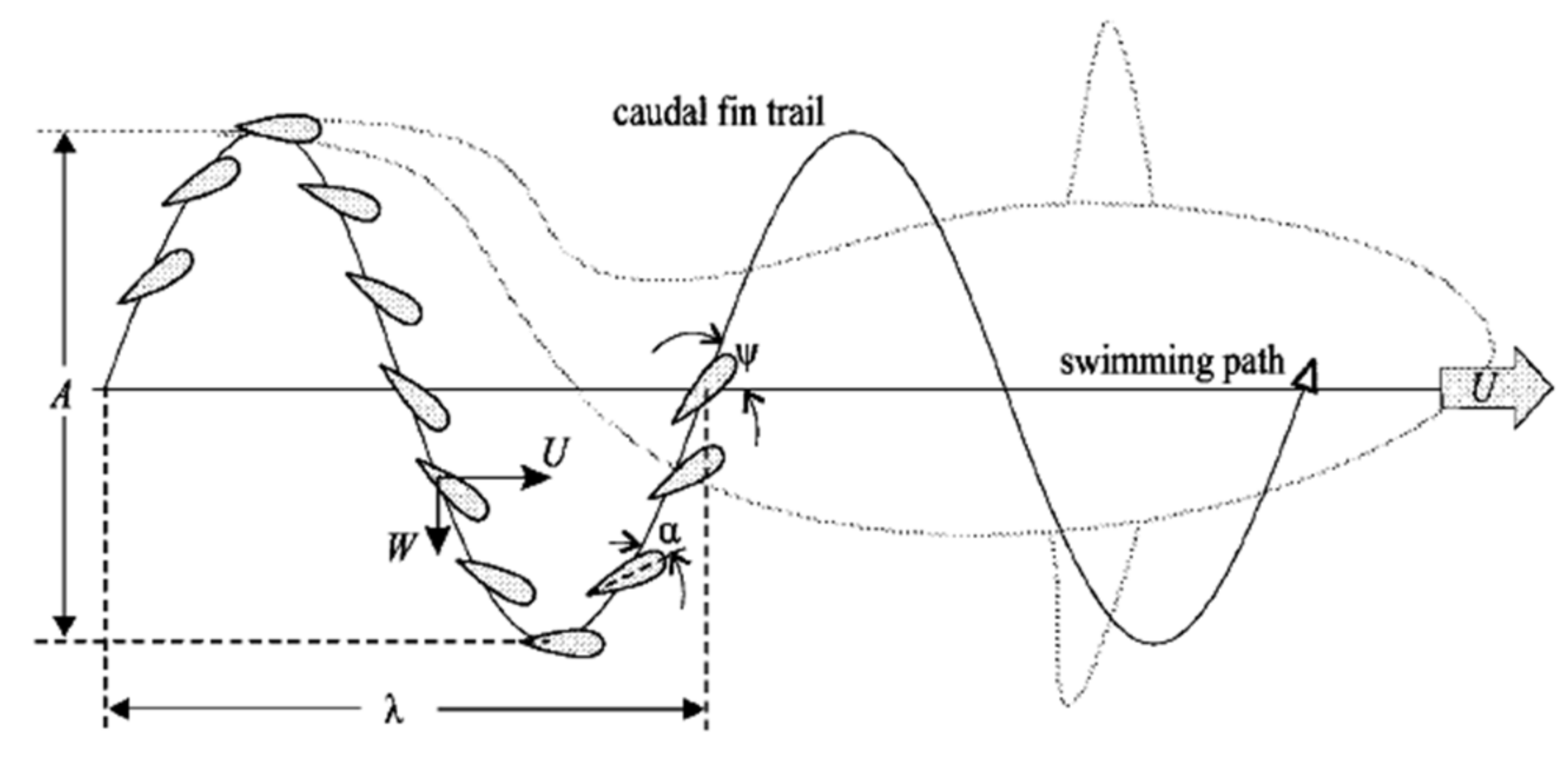
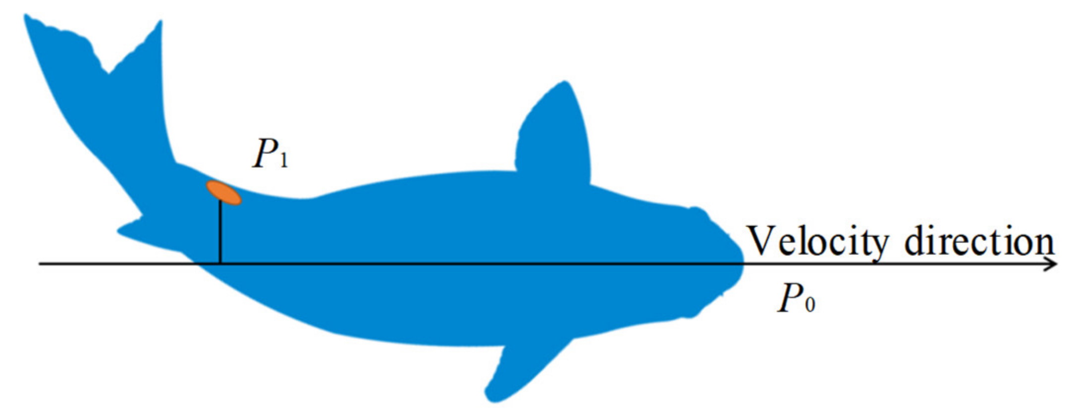
4.2.1. Kinematics Description of Fish

The general model of freshwater fish is in accordance with the push model of the carangidae. It is Illustrated by the example of bream, the body structure of which is shown in Figure 6. Along the longitudinal axis of body, the bream can be divided into three parts: the head, the trunk and the tail. When swimming, the head and trunk swing is small, and the propulsion movement is completed mainly by the tail.
According to Videler’s experiment [23], the propulsion movement consists of two parts: the body’s fluctuation and the caudal fin translational swing. The movement of caudal fin is shown in Figure 7 [24].
Thus, the kinetic model can be established. If we consider the longitudinal direction of fish body as the X-axis and the lateral direction of body as the Y-axis, the body fluctuations can be described as:
y b x , t = A 2 sin ω t k x = c 0 + c 1 x + c 2 x 2 sin ω t k x
where x is the longitudinal displacement of the body, A is the amplitude of the caudal fin movement, y b x , t   is the lateral displacement of body fluctuation of position   x at time   t , and ω , k   are the wave angular frequency and wave number of body, respectively.
The swing movement of caudal fins can be described as:
y c f t = H sin ω t k L b θ t = tan 1 H ω / u α m a x sin φ sin ω t k L b φ
where L b , α and φ are, respectively, the length of the fish, the strike angle, that is, the included angle between the swing axis and the center line of caudal fin, and the translational swing phase.

4.2.2. Improved Adaptive Kalman Filter

According to the body structure and movement model of the fish, it can be seen that, if the markers are attached to the fish, the swing amplitude of the fish side line is the largest, and the upper and lower areas of the line position are consistent with the movement frequency, and the fish body is symmetrical with respect to the dorsal fin. If the points are symmetrical, then their relative position does not change. Therefore, there is a constraint relationship between the position of the markers.
The number of vertebrae of Chinese Cypriniformes is 30 to 52, with an average of 39.5 ± 4.4. Assuming that the maximal angle between the two vertebrae is 2°, then the two markers M and N satisfy the following relationship:
M k 1 N k 1 ¯ , M k N k ¯ < 2 l L i
where M k 1 N k 1 ¯ and M k N k ¯ are, respectively, the connection of marker M, N of last and current frame, l represents the actual distance between two markers, L is the fish length, and i is the number of vertebrae.
Meanwhile, the marker is attached to the fish body and its movement is inseparable from the whole, whereas the integrated movement can also be obtained by the markers movement. Hence, to improve the prediction effect, the Kalman filtering results of the markers are corrected based on overall movement information, as shown in Figure 8.
Therefore, Kalman filter can be improved as
X ^ k | k = X ^ k | k 1 + K k Z k H X ^ k | k 1 + β M ^ k | k 1
where M ^ k | k 1 the is the estimation of the overall movement of fish and is the estimated coefficient of the overall motion.
Figure 9 shows the spatial position and the position after Kalman filtering of a marker in the live fish experiment, where the blue one indicates the measurement position and green one indicates the position processed with adaptive Kalman filtering.

5. Error Analysis and Correction

In order to measure the accuracy of the underwater 3D reconstruction, we fix the calibration plate and establish the world coordinate system at the current position of it, then pour the water into the tank until the water level is higher than the height of the calibration plate. Subsequently, the calibration plate corners are reconstructed, and its spatial positions are obtained. Finally, the error of the underwater 3D reconstruction can be obtained by comparing the actual position with the position derived from combining different cameras.

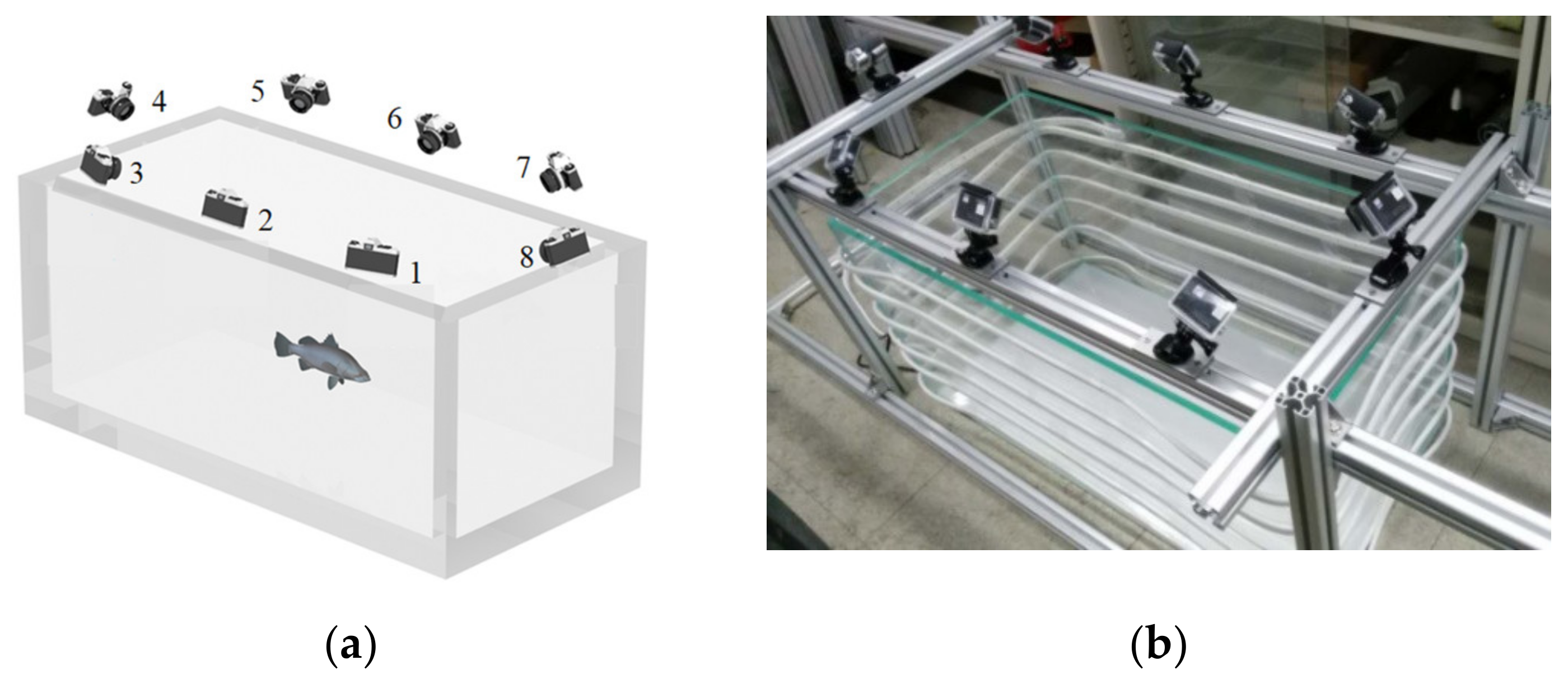
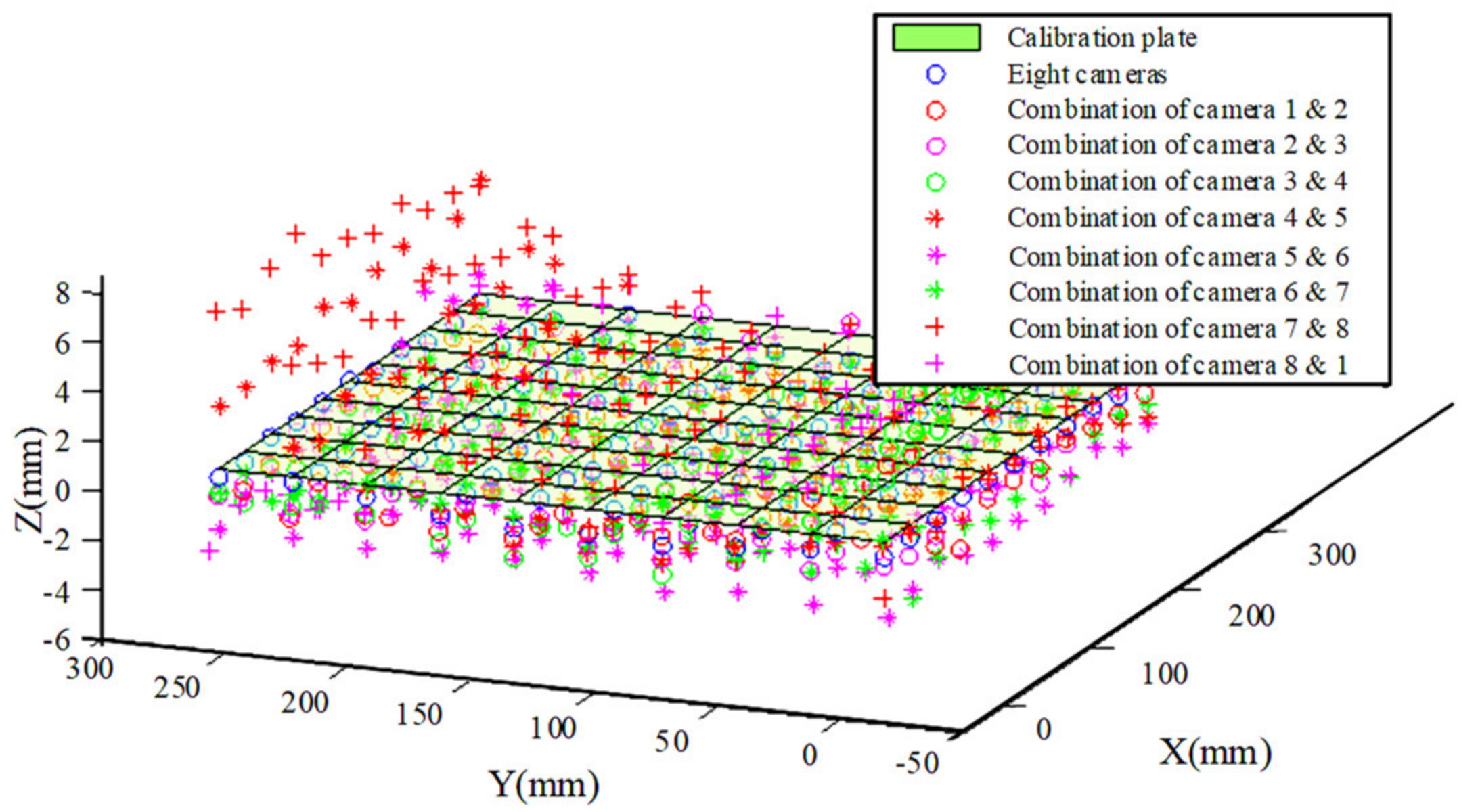
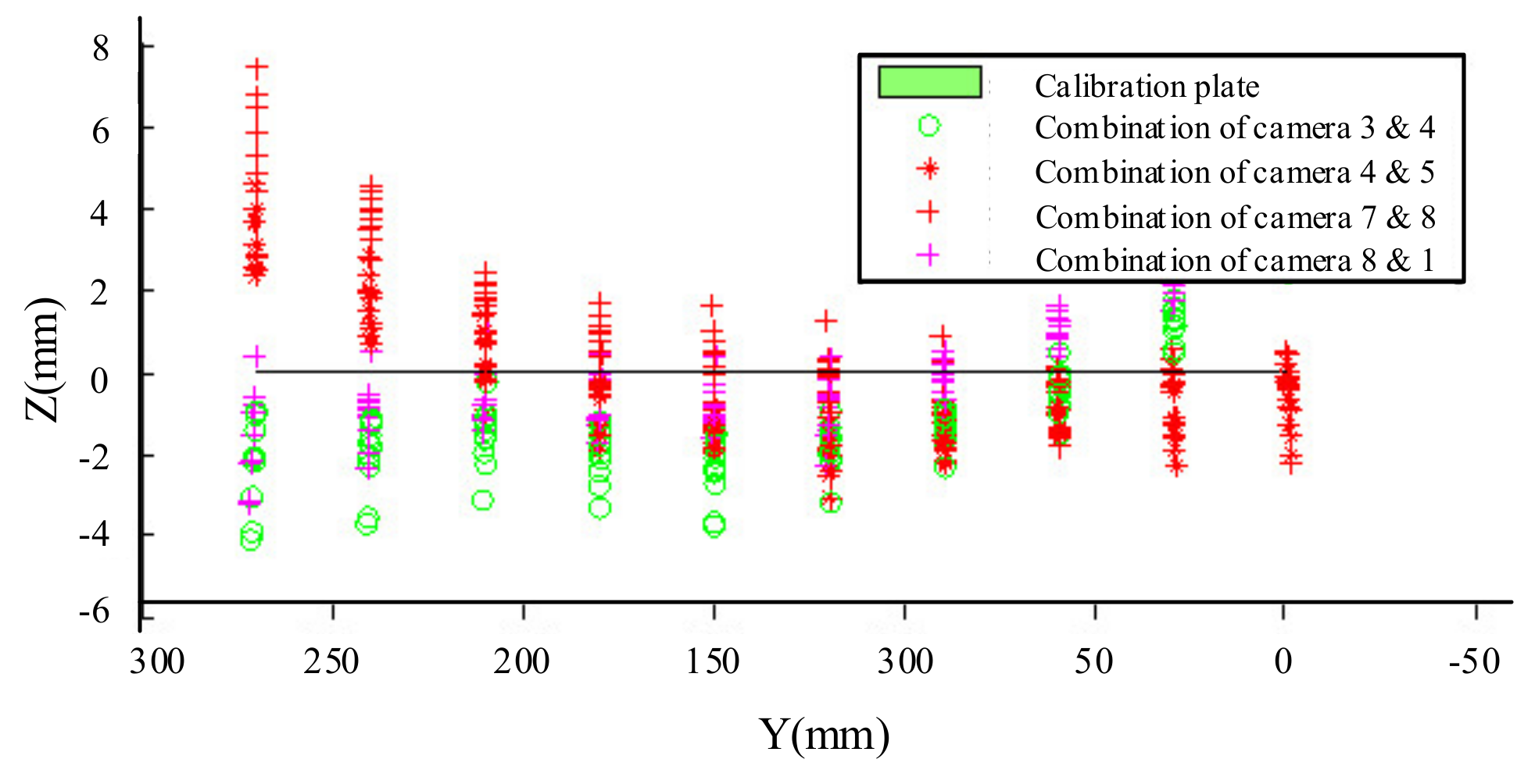
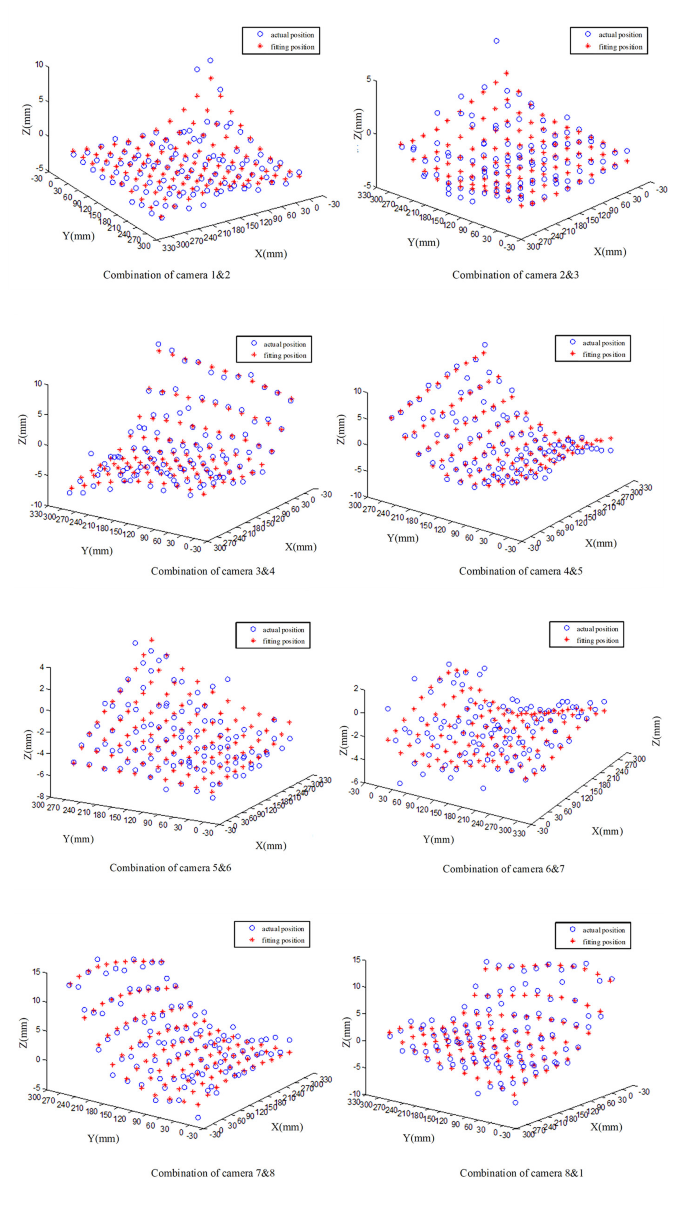
5.1. Reconstruction Experiment

In order to capture the movement information of fish and meet the image clarity, a fish tank with size of 1 m by 0.5 m by 0.5 m, with a surrounding LED strip, is used and eight numbered cameras of GoPro Hero4 with an image resolution of 1980 by 1080 and frame rate of 120 fps are fixed on an aluminum alloy bracket in the peripheral area, three of which are arranged on the long side and one is arranged on the short side. The overall experimental platform is shown in Figure 10. It should be noted that the distribution of eight cameras are centrosymmetrical to enable shooting with a wider range.
For the underwater error analysis, we fixed the calibration plate at the bottom of the fish tank and shot it from the air by the fixed camera, which set the world coordinate system with the plane of the calibration plate as Z = 0. Then we poured the water into tank, measured the water depth, and shot again. After that, the calibration plate corner can be reconstructed based on the underwater 3D reconstruction theory mentioned above. Figure 11 shows the result of underwater 3D reconstruction with water depth of 206 mm. The green plane in the figure represents the plane of the calibration plate and the positions of the intersection points are the actual positions of the calibration plate corners. It can be seen that combinations with a large error of underwater 3D reconstruction includes camera 4 and 8.
Figure 12 shows the positions of the reconstruction points of above partial combinations in the Y-Z plane, the reconstruction points are tilted at both ends of the Y axis, and cameras 5 and 7 are arranged in the positive direction of the Y axis, while cameras 1 and 3 are arranged in the negative direction of Y-axis, that is, the location where tilt is close to the camera.
By analyzing the error of 3D reconstruction in water and in the air, we can find that the error in the water is significantly larger than that in the air. The reasons for this are as follows:
(1)
The principle of underwater 3D reconstruction is to determine the intersection of the optical path and the water surface with the position of camera and marker and to solve the position with least squares method based on the intersection, which weakens the ability of least squares method to reduce the error.
(2)
Because of the accuracy of process and other issues, the plane of calibration plate and the water surface can only be approximately parallel, which introduces error simultaneously.
(3)
As we all know, the error increases as the distance of the point and camera increase.

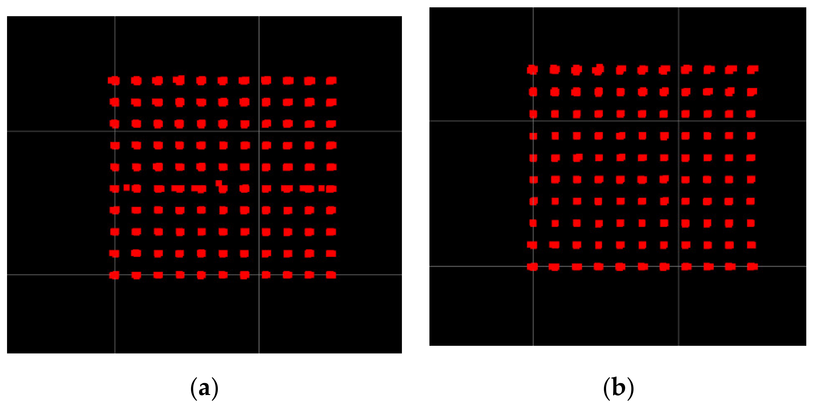
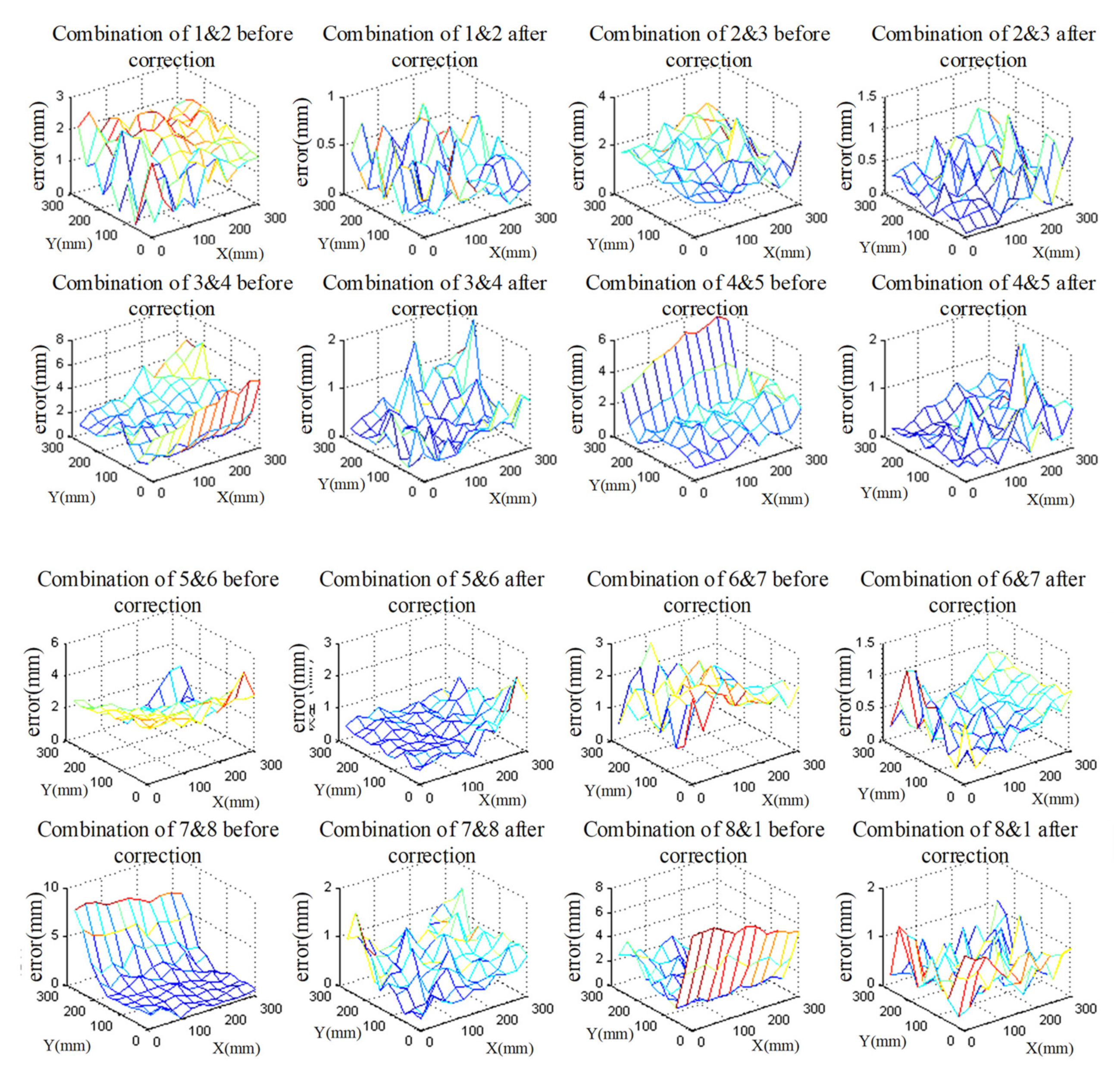
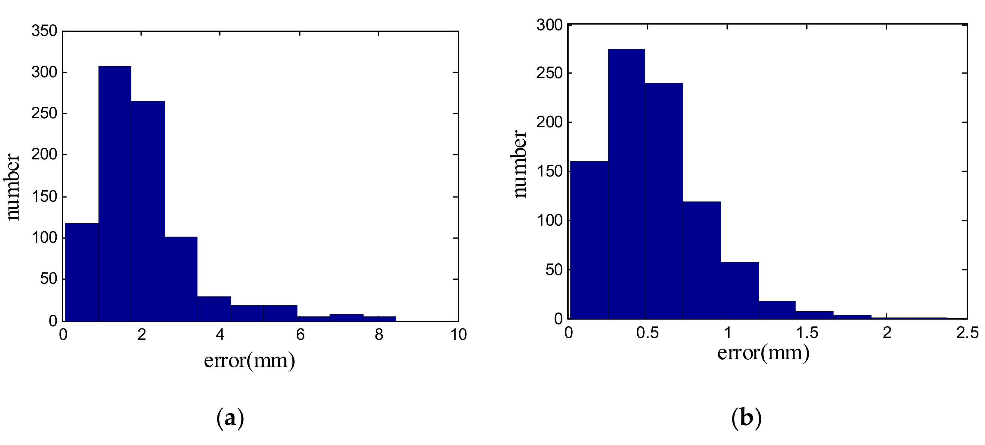
5.2. Correction of 3D Reconstruction

5.2.1. Normalization

In this paper, Equation (9) and the least squares method are used to calculate the underwater 3D reconstruction position. Moreover, the λ   in Equation (9) is related to the camera position and the intersection of optical path of physical point and water surface. When y w is approximately equal to y c , λ will be very large. While the principle of least squares method is to minimize the sum of the squares of error, if the weighting of a term is too large, the measured point will be tilted to it.
Therefore, we use the normalization method to correct Equation (9) and the corrected equation is as follows:
1 1 + λ 2 λ 1 + λ 2 0 x w + λ y w 1 + λ 2 0 1 γ λ 2 + 1 1 γ λ 2 + 1 + γ γ 1 γ λ 2 + 1 + γ 1 γ λ 2 + 1 y w + γ z w 1 γ λ 2 + 1 + γ x m y m z m 1 = 0 y m y w 1 1 + λ 2 λ 1 + λ 2 0 x w + λ y w 1 + λ 2 0 1 γ λ 2 + 1 1 γ λ 2 + 1 + γ γ 1 γ λ 2 + 1 + γ 1 γ λ 2 + 1 y w + γ z w 1 γ λ 2 + 1 + γ x m y m z m 1 0 y m > y w
After the normalization, the error when y w is approximately equal to y c is significantly reduced. Figure 13 shows the results of 3D reconstruction before and after normalization, it can be seen that when y is equal to about 120 mm, 3D reconstruction of the point is deviate from the actual position, while the deviation has been amended after normalization.

5.2.2. Correction Function

According to underwater 3D reconstruction theory, it can be deduced that the error is related to the water height, the camera position, and the marker position. Therefore, the following equation can be established to fit the Z-axis error:
z f i t = k 0 + k 1 x + k 2 y + k 3 x 2 + k 4 x y + k 5 y 2 + k 6 x 3 + k 7 x 2 y + k 8 x y 2 + k 9 y 3
where k i = g i 0 + g i 1 x c 1 + g i 2 y c 1 + g i 3 x c 2 + g i 4 y c 2 + g i 5 x c 1 2 + g i 6 y c 1 2 + g i 7 x c 2 2 + g i 8 y c 2 2 , x , y , z is the position of underwater 3D reconstruction, x c 1 , y c 1 , z c 1 and x c 2 , y c 2 , z c 2 are the positions of two cameras, which constitute the 3D reconstruction, in world coordinate system. The g i j is the ith coefficient of k i . The fitting results are as shown in Figure 14:

5.2.3. Results Verification

The verification method is as follows: fixing the calibration plate and verifying the validity of parameters of correction function at different water surface height. Figure 15 shows the comparison of errors before and after correction of the adjacent camera and we can see that the error is greatly reduced.
It can be concluded that before calibration, the maximum error is 8.45 mm and the average error is 2.06 mm and after correction, the maximum and average error are, respectively, 2.37 mm and 0.53 mm. The error distributions are shown in the Figure 16 and It is obvious that the error is significantly reduced after correction.

6. Experimental Results and Discussions

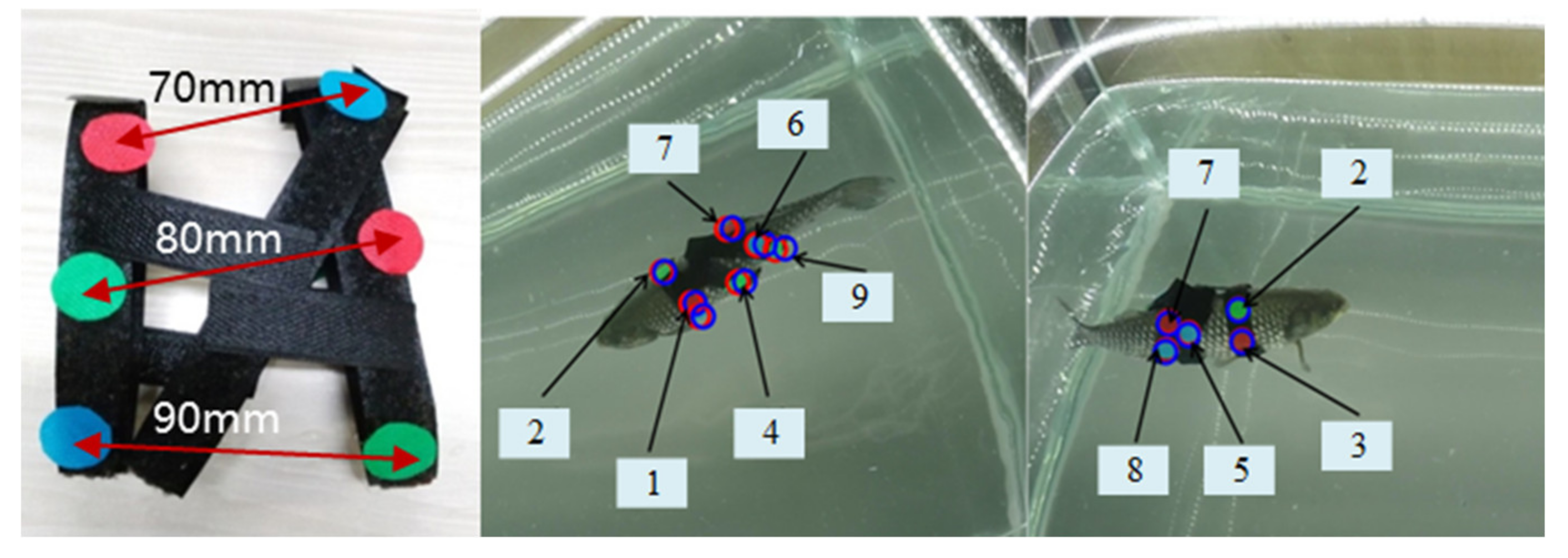
6.1. Implementation Settings
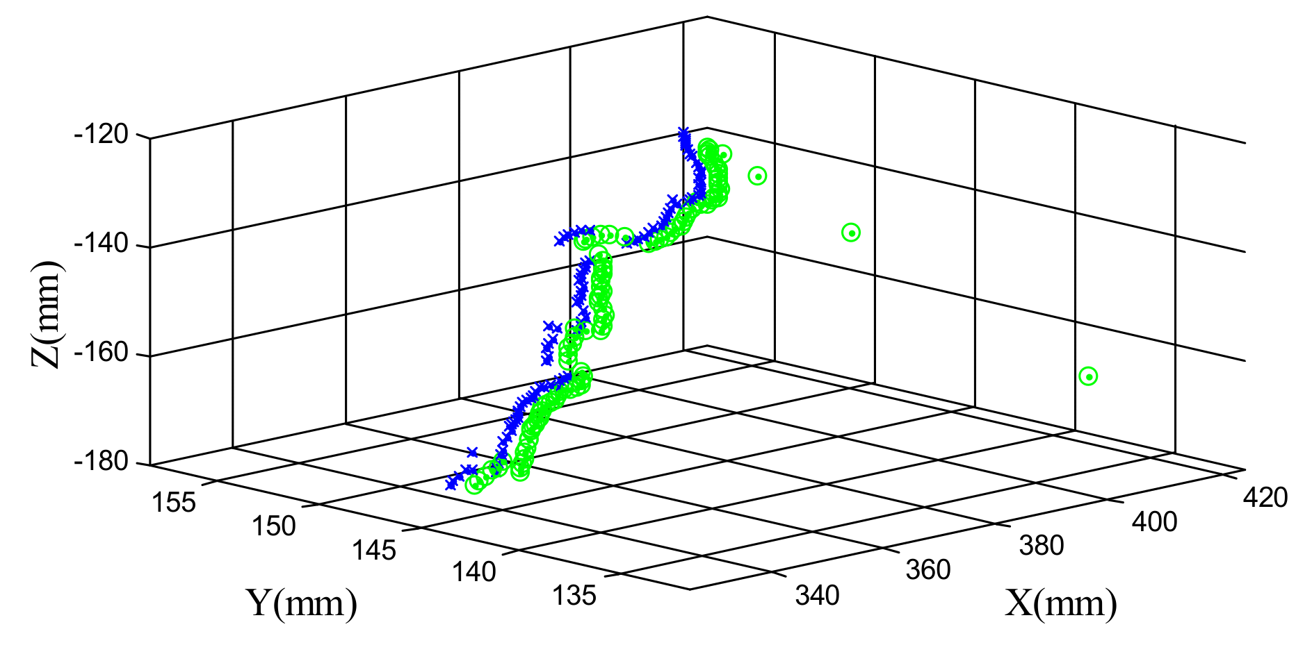
In this experiment, a carp about 0.5 kg that tied with 2 cm Velcro stuck with numbered markers is used as the experimental object. We numbered the markers attached to the fish and sorted it from the head to the tail. Figure 17 shows the pictures taken by camera 1 (left) and camera 5 (right) respectively, where marker 1 to 3 are located in the front part of the fish, 4 to 5 are located in the middle part of the fish, and 6 to 9 are located in the back part of the fish.
Based on the key technology of multi-media motion capture, we use Visual Studio, OpenCV, OpenGL, DataBase and other tools to design and develop its software system for achieving the camera calibration, motion capture, 3D display and other function. The system adopts modularization design and it is divided into six modules: log, auxiliary function, calibration, correction, 3D reconstruction and 3D display. The system structure and the software interface are shown in Figure 18 and Figure 19 respectively.

6.2. Data Analysis

After setting the world coordinate system, it starts the 3D reconstruction experiment of live fish: capturing the video of fish with 8 cameras simultaneously and reconstructing the markers attached to the fish body based on the image information with homemade motion capture software. The reconstruction result is shown in Figure 20. It displays the spatial positions of markers after 3D reconstruction taken from 0 to 700 frames with 100 frames separated, and the corresponding frame numbers by camera 6 with appropriate angle, where all markers are covered, is chosen as the comparison.
According to the previous experimental data, we can get the motion trail of fish, which is shown in Figure 21, it can be seen from the picture that the tracks of marker 1 to 3 are relatively stable, while the tracks of markers 4 to 9 swing with a certain degree, and this is consistent with the swimming model of the Carangidae that the propulsion force is mainly caused by tail swing.
Because fish swimming is a dynamic process, we take the relative movement between markers on the fish tail and markers on the front part of fish as a study object and select the motion direction of markers 1 to 3 as the motion direction of the fish. Then, the relative motion direction of each marker can be obtained, that is adjusting the overall fish swimming to the swimming along the X axis and observing the position of marker relative to it. As shown in Figure 22, the position P 0 and velocity direction can be determined by the marker 1 to 3. The position of each marker in the relative speed direction is the shortest distance from the axis of P 1 to P 0 .
Figure 23 shows the distances between each marker and the axis, it can be seen that the markers of 5, 7, and 8 are similar in motion, all of which belong to the same side. Near the 50th frame, the motion direction of these three markers is opposite to that of the other four markers, which is because the axis is in the middle of the two markers sets; the markers on one side are away from the axis and the markers on other side must be close to the axis. At the same time we can see that when the fish is suspended in the water at 500th frame, the markers of 5, 7 and 8 are farthest from the axis, this because the markers of 1 to 3 are chosen as the basic markers, which leads to the result that the axis will be tilted to this side and the markers of the other side are farthest from the axis. Observing the data from 0 to 200 frames, it can be seen that the movement of the fish tail is similar to the sinusoidal motion, which also conforms to the tail swing of the carangid in Formula (21).
Because of the limitation of the experimental conditions, the system errors in our experiment are obtained by comparing the relative distances of calibrated markers which are arranged as in Figure 17. In order to achieve accurate results, both the motion of translation and rotation are analyzed, and the results are shown in Figure 24. The maximum error in translational motion is 3.84 mm, and the maximum error during rotation is 3.22 mm, which indicates that the error between the measured value and actual value is small.

7. Conclusions

In order to explore the locomotion patterns and swimming modes of fish for improving the swimming performance of bionic robot-fish, a multi-medium motion capture system based on markers is developed in this paper. Initially, a multi-medium 3D reconstruction model is established through the least square method. Due to the multi-colored markers used in system, there will be more than one of same colored markers in same frame by different cameras. Therefore, it is necessary to match the same colored markers. We firstly match the markers in the first frame according to the flat structure of the fish, amd subsequently, with the constrains of fish speed and others, we match the markers in subsequent frames, then accomplish it through the K-means clustering algorithm. Furthermore, because of the shooting angle limit and fish movement, there are some markers that are occluded or only captured by one camera, which cannot be reconstructed. To solve this, we adopt the mean-variance adaptive Kalman filtering algorithm and add the overall swimming information of the fish in it according to its kinematics model for improving the prediction effect. Finally, through the experimental method, the kinematics model of the fish swimming is verified and the feasibility as well as effectiveness of the proposed system are demonstrated. The main models and methods of this paper can provide a reference and inspiration for the measurement of underwater objects.

Author Contributions

Conceptualization and methodology Z.Z. and X.L.; validation, and formal analysis, Z.W. and L.H.; software, S.X.; writing—original draft preparation, L.H. and X.L.; writing—review and editing, Z.Z. and Z.W.; project administration and funding acquisition, Z.Z. and B.H. All authors have read and agreed to the published version of the manuscript.

Funding

This research was funded in part by Shanghai Zhangjiang National Independent Innovation Demonstration Zone Special Development Fund Major Project Plan, grant number ZJ2019-ZD-003, in part by National Postdoctoral Program for Innovative Talents, grant number BX20190243, in part by National Natural Science Foundation of China (Grant Nos. 51975415 and 61825303), and in part by the Fundamental Research Funds for the Central Uniersities (No. 22120180562).

Acknowledgments

The author wishes to thank the editor and the reviewers for their contributions on the paper.

Conflicts of Interest

The authors declare no conflict of interest.

References

  1. Liang, J.; Wang, T.; Wen, L. Development of a two-joint robotic fish for real-world exploration. J. Field Robot. 2011, 28, 70–79. [Google Scholar] [CrossRef]
  2. Fei, S.; Changming, W.; Zhiqiang, C.; De, X.; Junzhi, Y.; Chao, Z. Implementation of a Multi-link Robotic Dolphin with Two 3-DOF Flippers. J. Comput. Inf. Syst. 2011, 7, 2601–2607. [Google Scholar]
  3. Ryuh, Y.S.; Yang, G.H.; Liu, J.; Hu, H. A School of Robotic Fish for Mariculture Monitoring in the Sea Coast. J. Bionic Eng. 2015, 12, 37–46. [Google Scholar] [CrossRef]
  4. Yu, J.; Wang, C.; Xie, G. Coordination of Multiple Robotic Fish with Applications to Underwater Robot Competition. IEEE Trans. Ind. Electron. 2016, 63, 1280–1288. [Google Scholar] [CrossRef]
  5. Junzhi, Y.U.; Wen, L.; Ren, Z.Y. A survey on fabrication, control, and hydrodynamic function of biomimetic robotic fish. Sci. China Technol. Sci. 2017, 60, 1365–1380. [Google Scholar]
  6. Thompson, J.T.; Kier, W.M. Ontogeny of Squid Mantle Function: Changes in the Mechanics of Escape-Jet Locomotion in the Oval Squid, Sepioteuthis lessoniana Lesson, 1830. Biol. Bull. 2002, 203, 14–16. [Google Scholar] [CrossRef] [PubMed] [Green Version]
  7. Conti, S.G.; Roux, P.; Fauvel, C.; Maurer, B.D.; Demer, D.A. Acoustical monitoring of fish density, behavior, and growth rate in a tank. Aquaculture 2006, 251, 314–323. [Google Scholar] [CrossRef] [Green Version]
  8. Stamhuis, E.; Videler, J. Quantitative flow analysis around aquatic animals using laser sheet particle image velocimetry. J. Exp. Biol. 1995, 198, 283. [Google Scholar]
  9. Meng, X.; Pan, J.; Qin, H. Motion capture and retargeting of fish by monocular camera. In Proceedings of the 2017 IEEE International Conference on Cyberworlds, Chester, UK, 20–22 September 2017; pp. 80–87. [Google Scholar]
  10. Yu, J.; Wang, L.; Tan, M. A framework for biomimetic robot fish’s design and its realization. In Proceedings of the American Control Conference 2005, Portland, OR, USA, 8–10 June 2005; Volume 3, pp. 1593–1598. [Google Scholar]
  11. Budick, S.A.; O’Malley, D.M. Locomotor repertoire of the larval zebrafish: Swimming, turning and prey capture. J. Exp. Biol. 2000, 203, 2565. [Google Scholar]
  12. Bartol, I.K.; Patterson, M.R.; Mann, R. Swimming mechanics and behavior of the shallow-water brief squid Lolliguncula brevis. J. Exp. Biol. 2001, 204, 3655. [Google Scholar]
  13. Yan, H.; Su, Y.M.; Yang, L. Experimentation of Fish Swimming Based on Tracking Locomotion Locus. J. Bionic Eng. 2008, 5, 258–263. [Google Scholar] [CrossRef]
  14. Lai, C.L.; Tsai, S.T.; Chiu, Y.T. Analysis and comparison of fish posture by image processing. In Proceedings of the 2010 International Conference on Machine Learning and Cybernetics, Qingdao, China, 11–14 July 2010; Volume 5, pp. 2559–2564. [Google Scholar]
  15. Pereira, P.; Rui, F.O. A simple method using a single video camera to determine the three-dimensional position of a fish. Behav. Res. Methods Instrum. Comput. 1994, 26, 443–446. [Google Scholar] [CrossRef]
  16. Viscido, S.V.; Parrish, J.K.; Grünbaum, D. Individual behavior and emergent properties of fish schools: A comparison of observation and theory. Mar. Ecol. Prog. 2004, 273, 239–249. [Google Scholar] [CrossRef]
  17. Zhu, L.; Weng, W. Catadioptric stereo-vision system for the real-time monitoring of 3D behavior in aquatic animals. Physiol. Behav. 2007, 91, 106–119. [Google Scholar] [CrossRef] [PubMed]
  18. Oya, Y.; Kawasue, K. Three dimentional measurement of fish movement using stereo vision. Artif. Life Robot. 2008, 13, 69–72. [Google Scholar] [CrossRef]
  19. Ham, H.; Wesley, J.; Hendra, H. Computer vision based 3D reconstruction: A review. Int. J. Electr. Comput. Eng. 2019, 9, 2394. [Google Scholar] [CrossRef]
  20. Jordt, A.; Köser, K.; Koch, R. Refractive 3D reconstruction on underwater images. Methods Oceanogr. 2016, 15, 90–113. [Google Scholar] [CrossRef]
  21. Liu, X.; Yue, Y.; Shi, M.; Qian, Z.M. 3-D video tracking of multiple fish in a water tank. IEEE Access 2019, 7, 145049–145059. [Google Scholar] [CrossRef]
  22. Ichimaru, K.; Furukawa, R.; Kawasaki, H. CNN based dense underwater 3D scene reconstruction by transfer learning using bubble database. In Proceedings of the 2019 IEEE Winter Conference on Applications of Computer Vision (WACV), Waikoloa Village, HI, USA, 7–11 January 2019; pp. 1543–1552. [Google Scholar]
  23. Videler, J.J.; Hess, F. Fast continuous swimming of two pelagic predators, saithe (Pollachius virens) and mackerel (Scomber scombrus): A kinematic analysis. J. Exp. Biol. 1984, 109, 209. [Google Scholar]
  24. Sfakiotakis, M.; Lane, D.M.; Davies, J.B.C. Review of fish swimming modes for aquatic locomotion. IEEE J. Ocean. Eng. 1999, 24, 237–252. [Google Scholar] [CrossRef] [Green Version]
Figure 1. Refraction model.
Applsci 10 06237 g001
Figure 2. Marker matching diagram considering the error.
Applsci 10 06237 g002
Figure 3. Markers matching flow chart.
Applsci 10 06237 g003
Figure 4. Marker forecast.
Applsci 10 06237 g004
Figure 5. Marker forecast processed by Kalman filtering.
Applsci 10 06237 g005
Figure 6. Description of bream body structure and shape.
Applsci 10 06237 g006
Figure 7. Caudal fins trajectories of carangidae.
Applsci 10 06237 g007
Figure 8. Kalman filter based on overall information of fish.
Applsci 10 06237 g008
Figure 9. Measuring position and filtered position of marker.
Applsci 10 06237 g009
Figure 10. Experimental platform. (a) The test bench layout diagram, (b) The picture of the real test bench.
Applsci 10 06237 g010
Figure 11. Underwater 3D reconstruction with combinations of adjacent cameras.
Applsci 10 06237 g011
Figure 12. Y-Z plane of underwater 3D reconstruction with partial combined camera.
Applsci 10 06237 g012
Figure 13. Results of 3D reconstruction (a) The result of 3D reconstruction before normalization, (b) The result of 3D reconstruction after normalization.
Applsci 10 06237 g013
Figure 14. Results of fitting error of combinations of adjacent cameras in Z-axis.
Applsci 10 06237 g014
Figure 15. Error of each camera combination before and after correction.
Applsci 10 06237 g015
Figure 16. Errors distribution, (a) Errors distribution before correction (b) Errors distribution after correction.
Applsci 10 06237 g016
Figure 17. Captured by camera 1 (left) and 5 (right).
Applsci 10 06237 g017
Figure 18. System structure.
Applsci 10 06237 g018
Figure 19. Software interface.
Applsci 10 06237 g019
Figure 20. D reconstruction results in software and pictures captured by camera.
Applsci 10 06237 g020
Figure 21. Marker movement trajectory.
Applsci 10 06237 g021
Figure 22. Fish swimming diagram.
Applsci 10 06237 g022
Figure 23. Distance between the markers and the axis.
Applsci 10 06237 g023
Figure 24. The system errors analysis of the relative distances of calibrated markers.
Applsci 10 06237 g024

