1. Introduction
Landslides are a major geological hazard, which can result in the loss of human life and economic damage, in many areas on Earth. According to the Centre for Research on Epidemiology of Disasters, landslides are responsible for 17% of the world’s natural hazard fatalities [
1]. To reduce damage from landslides, many scientific studies have sought to predict landslide occurrence and evaluate runout distances. Landslide prediction research has used both physically based landslide susceptibility methods and probabilistic analysis methods. Physically based landslide susceptibility assessment methods usually base a landslide initiation model on the physical properties of the soils and rocks on slopes and so predict slope instability [
2,
3,
4,
5,
6,
7,
8,
9,
10]. In probabilistic analysis methods, several parameters are considered as random variables and the statistical parameters and probability density functions of uncertain variables are estimated [
8,
11,
12,
13,
14,
15,
16,
17,
18,
19,
20,
21]. Using soil, rock, and slope maps, such analysis can identify areas of high landslide potential within a regional area. Several statistical methods can be used in probabilistic analyses to evaluate landslide susceptibility. Among these, logistic regression analysis is commonly used because its results are considered the most reliable [
22,
23,
24,
25,
26]. Logistic regression is a useful method, and applicable to landslide occurrence, when the dependent variable is categorical, and the independent variables are categorical and/or numerical. According to [
27], logistic regression has been chosen for many studies because: (i) it is one of the most common statistical methods used to model landslide susceptibility, (ii) logistic regression has the lowest rate of error, increasing confidence in the results of any comparison, (iii) logistic regression generates a statistical significance value for each covariate in the model, and (iv) logistic regression estimates probabilities of landslide susceptibility and hazard.
For landslide damage assessment, landslide runout has been modeled based on topography, the properties of the slide materials, and soil water content. Fast landslides, such as debris flows, tend to accelerate below the initial failure, and when their displacements are of high volume, they can cause critical damage, and many casualties, in the area hit by the landslide. This makes the prediction of landslide runout necessary to encourage preparedness and reduce damage. Many studies have sought to model landslide runout by considering the properties, volumes, and mobilities of the moving materials [
28,
29,
30,
31,
32,
33,
34,
35].
Since 2000, in the Korean Peninsula, the number of landslide events on natural terrain has increased continuously under the influence of increasing rainfall amounts and durations as a consequence of climate change. Considering the seriousness of landslide hazards in Korea, this study analyzed landslide susceptibility and simulated debris flows runout distances near a construction site in Chooncheon, Korea. Many landslides occurred in Chooncheon in July 2011 and July 2013 resulting in huge damage to local people and their properties. Community infrastructure was planned at the construction site at the bottom of a mountain necessitating a comprehensive evaluation of the safety of the facility. Therefore, to estimate the likelihood of damage to the site, this study used a landslide prediction map of the area, which had been drawn in 2008 with a logistic regression model suggested by [
14], to determine landslide susceptibility. The authors then simulated debris-flow runout distances in the major watersheds around the construction site. There have been few prior runout distance modeling studies in Korea and prediction of runout distances is rare. An exception is the Debris-2D model [
36,
37] for simulation of runout distances under Korean geologic and topographic conditions. Debris-2D was therefore used for this study.
2. Distribution of Regolith in the Study Area
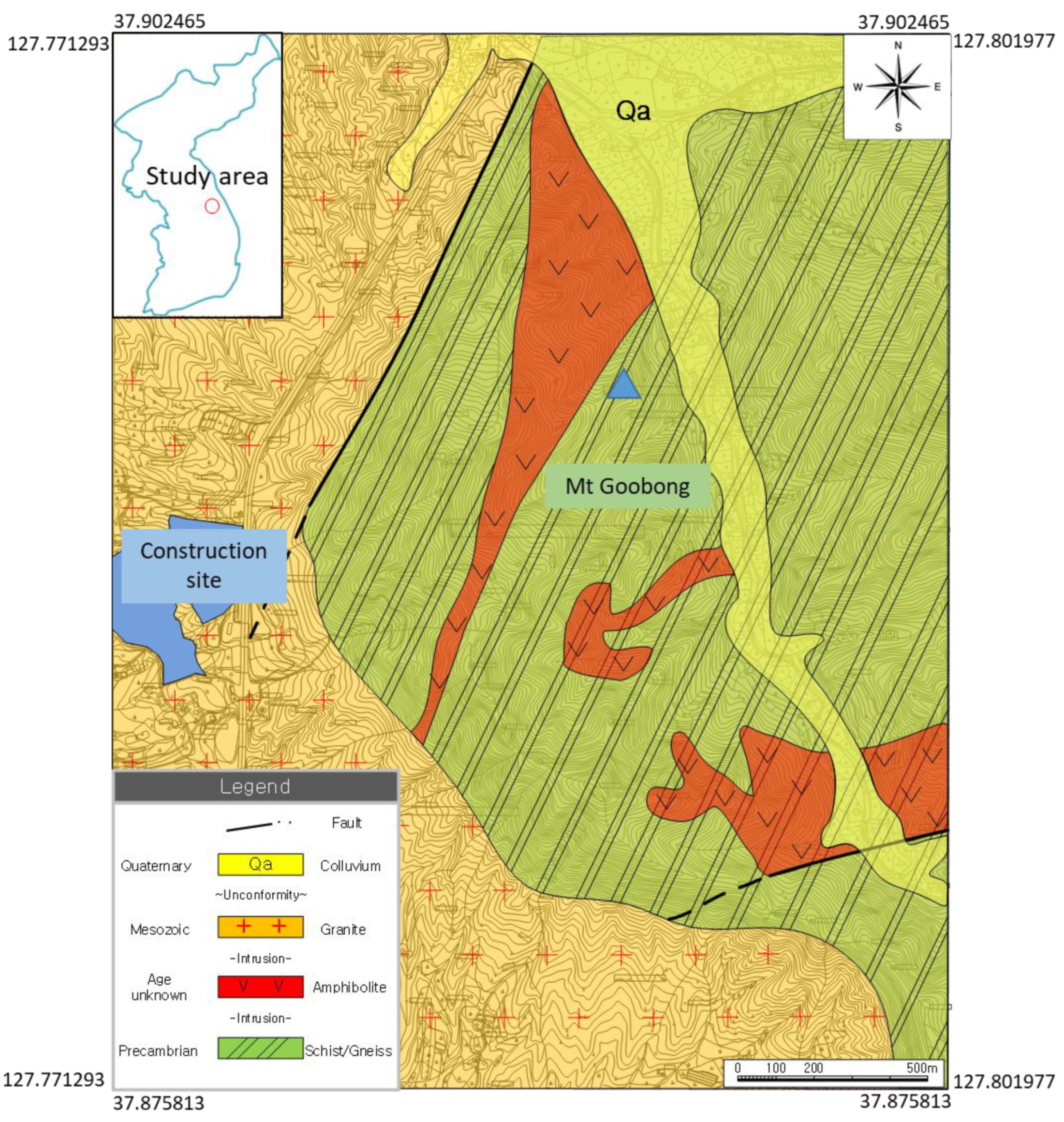
The geology of the study area includes a Precambrian gneiss and schist complex, age unknown amphibolites, Mesozoic granites, and Quaternary colluvium. The gneiss and schist complex and the amphibolites are the major lithologies of Mt Goobong. The Mesozoic granites, with highly weathered features, are distributed in the western part of the study area (
Figure 1).
The amphibolites are distributed only in Mt Goobong. The intrusion direction is N10-20E on the western part of the mountain. According to the field investigation, the amphibolites are exposed as about 20m in width on the western part of Mt Goobong. The Mesozoic granites are distributed in the western part of the survey area including the construction site. Because the granites are more susceptible to weathering, it is difficult to find granites outcrops in the field.
When the granites were intruded into the gneisses and schists in the area, the intrusion occurred along a fault with NE orientation. The boundary between the granites and the gneisses and schists complex shows linear feature. There is another fault with N10E orientation and higher density of fractures near the boundary. It indicates that the boundary between the granites and the gneisses and schists complex is thought to be a fault contact. Since the areas occupied by the granites have low elevation and gentle slope angle in the study area, it was easy to recognize lithological boundary showing marked difference of slope gradient and elevation in the field survey. According to the results of core logging in the construction site composed of the granites [
38], depth of boundary between weathered rock and weathered soil show various distribution from 6.0 m to 18.5 m below ground surface. The difference of weathering depth in the granite area has been explained by Migon [
39]. The progress of weathering vertically is controlled by the pre-existing structure of rock, its mineralogy, and the discontinuities. Because granites usually have difference of weathering depth and extent, the thickness of the saprolite may be highly variable. On the other hand, the boundary between weathered rock and weathered soil is distributed from 1.0 m to 1.5 m below ground surface in the metamorphic rock area of the study area.
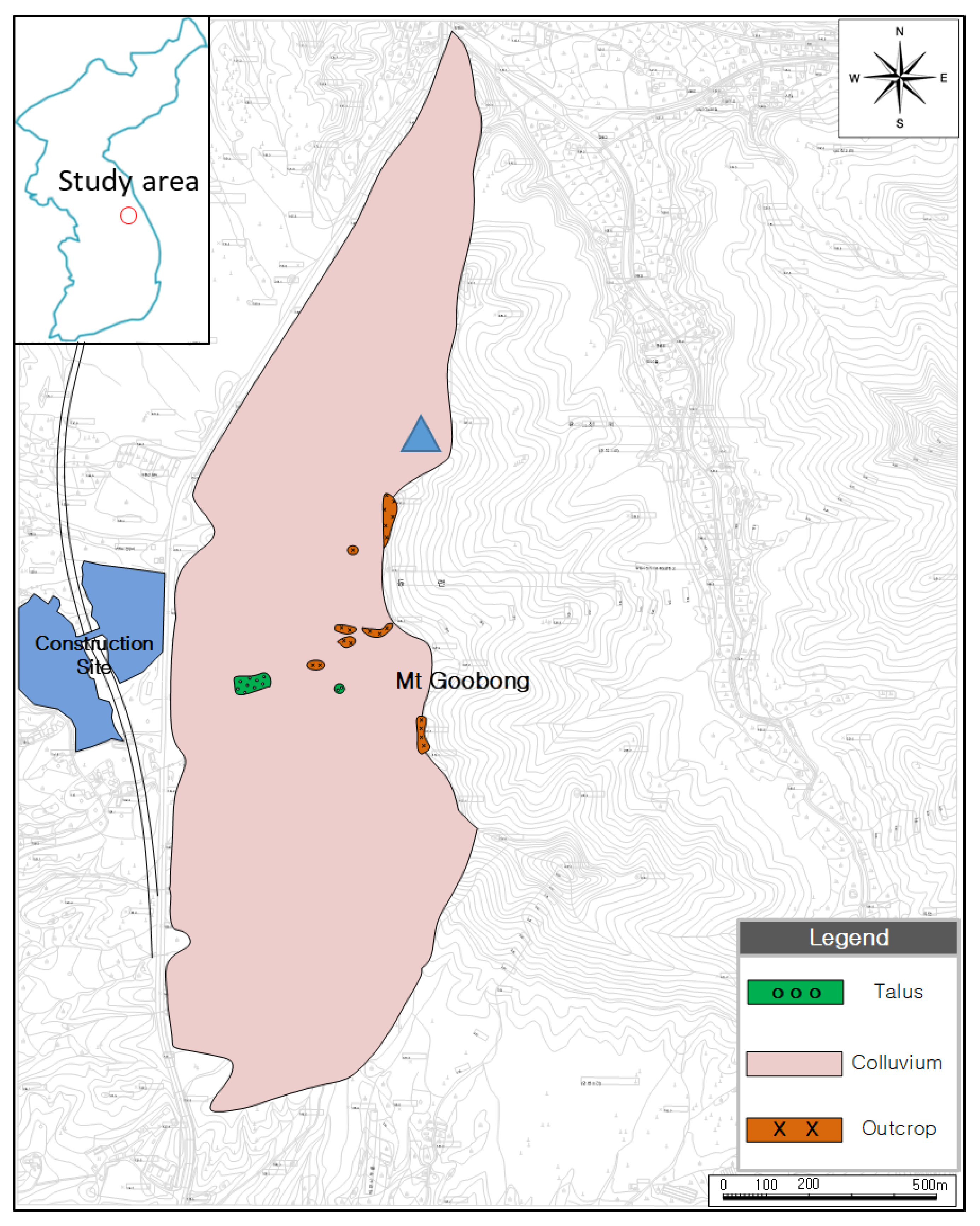
This study undertook field mapping of regolith distribution. Regolith is unlithified material distributed over bedrock. The field mapping was performed at the western part of Mt Goobong and the construction site based on a classification of regolith suggested by [
40] (
Table 1). The authors classified regolith on the surface and measured areal distribution and vertical thickness of regolith in the field. The Mt Goobong area is primarily composed of outcrops, residual colluvium, and talus (
Figure 2). The outcrops are gneisses and schists whose exposure is limited to near the top of the mountain (
Figure 3). Although the mountain has steep slope angles, of 30–40 degrees, outcrops are only exposed in very small areas on the mountain.
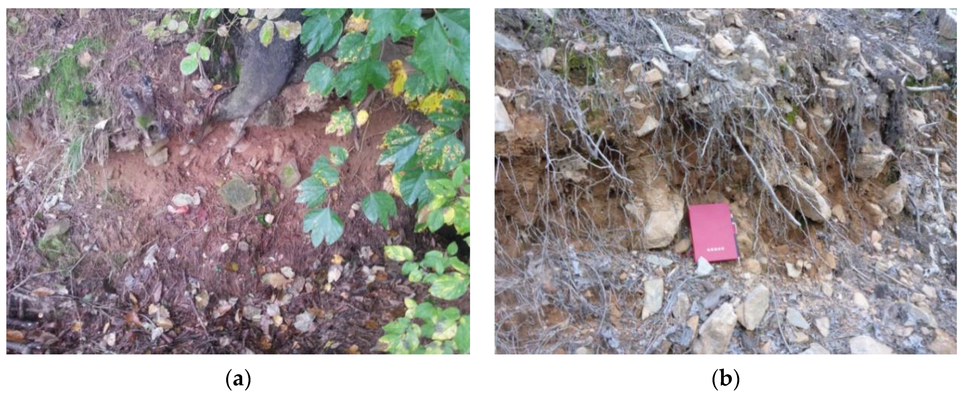
The residual colluvium is broadly distributed on Mt Goobong with a thickness of 1.0–1.5 m as observed in trenches and soil cross sections. They are composed of angular cobble size of rock fragments, clayey silts, and sandy silts (
Figure 4). On the mountain slopes, the residual colluvium has relatively similar thickness averaging 0.5 m near the top of the mountain. This thick residual colluvium, on steep slopes, can produce high volume landslide debris flows.
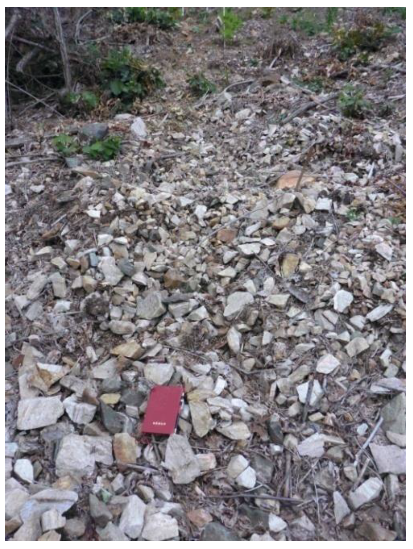
Talus has a limited distribution on the mountain slope (
Figure 5). Talus is generally formed by disintegration and collapse of highly fractured and weathered rock masses. The average size of rock fragments in talus is cobble size, of the order of 10 cm × 10 cm, in this area. This indicates that metamorphic rock masses such as gneisses and schists have detached to rock fragments under weathering along foliations and joints.
3. Method of Numerical Simulation of Debris Flows Based on Landslide Susceptibility Analysis
The Chooncheon landslide events of 2011 and 2013 suggest that further landslides and related debris flows are likely in the future under heavy rainfall. To reliably assess the potential damage from landslides and debris flows, it is necessary to assess both landslide susceptibility and the behavior of debris flows. Since the major objective of this study was to assess the safety of the construction site, relative to debris flows from Mt Goobong, numerical simulation was used to predict the runout distance of debris flows under the scenarios based on the results of landslide susceptibility analysis. Accurate simulations of debris flows require landslide information such as initiation locations and the amount of debris transported from the source areas. Therefore, this study analyzed landslide susceptibility, using a landslide prediction map, and then simulated debris-flow runout distances from areas of high landslide probability. This process improved the accuracy of debris volumes in upper mountain areas and increased the reliability of debris runout distances at the bottom of the mountain.
3.1. Analysis of Landslide Susceptibility
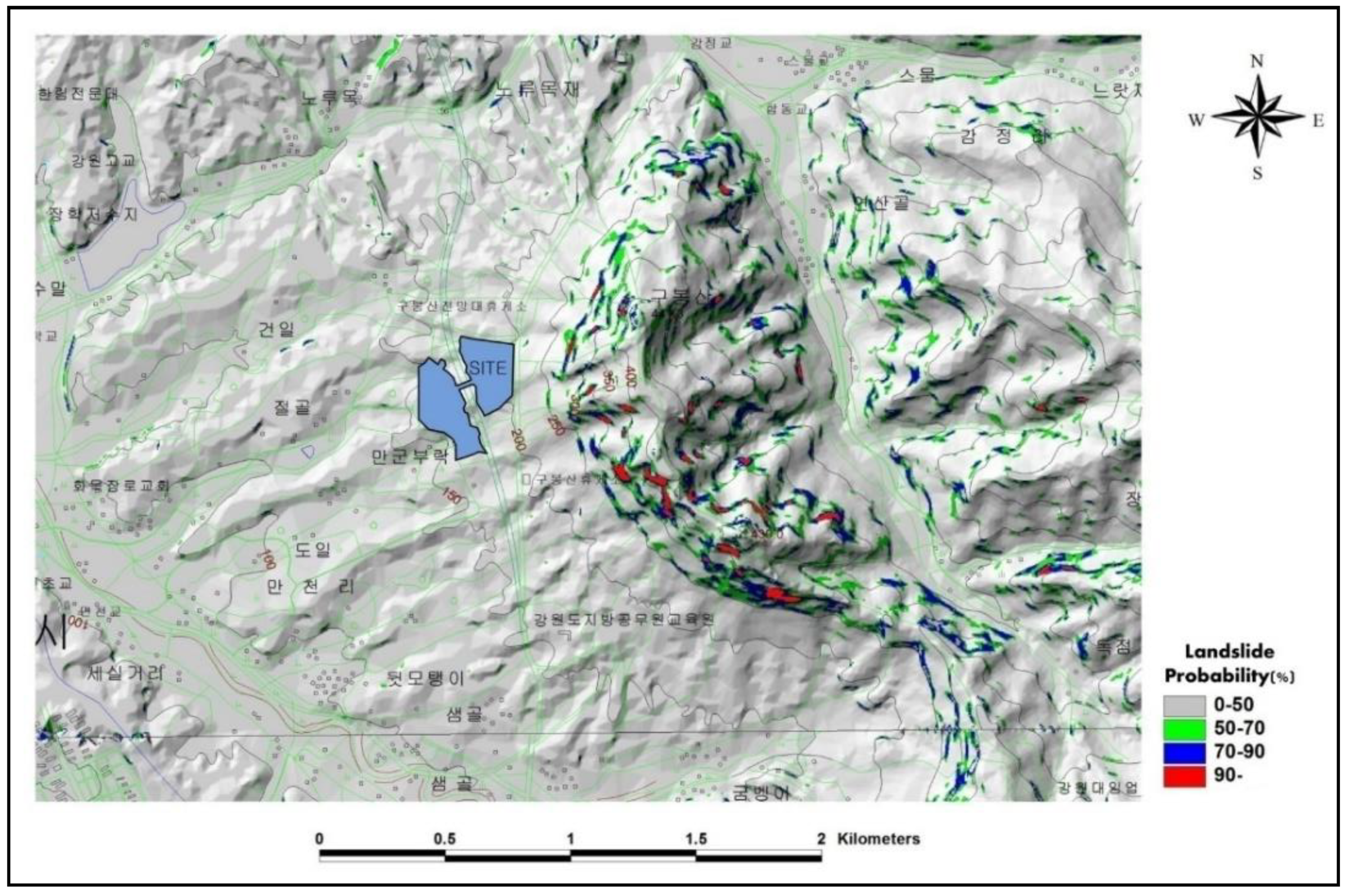
Landslide susceptibility was analyzed based on the landslide probability mapping of the area by [
11]. The landslide probability map was drawn by using a logistic regression model, developed by [
14], to predict landslide susceptibility. The target area of landslide prediction was Mt Goobong, located to the east of the construction site. The metamorphic rock complex, amphibolites and colluvium, 1.0–1.5 m thick on slopes of 30–40 degrees, make the mountain susceptible to landslides.
Chae et al. [
14] proposed a logistic regression landslide model reflecting the complex relationship among the factors (especially geology, topography, and soil properties) influencing landslides. The following is the logistic regression model for landslide prediction derived by [
14].
The output of this equation is converted to probability with the following equation.
Chae et al. [
11] used this relationship for landslide prediction mapping in the Chooncheon area including Mt Goobong. Among the factors in Equation (1), slope angle and elevation were collected by the topographic digital elevation model (DEM). Lithology was classified by a field survey for the study area. Soil properties such as dry density, permeability coefficient and porosity were acquired by the laboratory soil tests with undisturbed soil samples collected at the field. The area was divided into 10 m × 10 m cells and factor values (as in Equation (1)) were assigned to each cell. The logit values were then calculated in each cell and converted to landslide occurrence probabilities. This landslide prediction map was used to assess the landslide susceptibility of the study area, covering 12 km
2, around Mt Goobong (
Figure 6).
Focusing on the western slope of the mountain, the probability of a landslide was grouped into four grades. Areas with over 70% landslide probability, when over 250 mm of rain fell locally in 24 h, were categorized as high potential based on [
14]. According to the rainfall data in Chooncheon area from 2000 to 2019, rainfall events over 250 mm/24 h occurred three times in 2011, 2013 and 2016. Because the most highly weighted factor in the logistic regression model is slope angle, landslide probability is primarily controlled by slope angle with steep slopes having higher landslide probabilities than gentle slopes. However, steep slope areas with outcrops, and hence fewer soil materials, tend to have landslide probabilities lower than 50%. The outcrop areas were determined during the regolith mapping on Mt Goobong.
Within the prediction map, areas with 70–90% landslide probability cover 3.5% of the land and those with over 90% probability are 0.79% of the area. The location of the construction site appears to be particularly vulnerable to debris flows from two valleys, both with areas of landslide probability over 70%. Other parts of Mt Goobong, to the north and south of the construction site, also include several areas with over 70% landslide probability.
3.2. Numerical Simulation of the Runout Distance of Debris Flows
This study used the program Debris-2D [
36,
37] to simulate debris flow. In Debris-2D the theory of viscoplastic fluid, which is a branch of non-Newtonian fluid mechanics, is applied to model debris motion. The bulk of debris flow is treated as a continuum. The governing equations are based on mass and momentum conservation, with a shallow water assumption. The coordinate system is Cartesian with the average bed elevation as the
x-axis. The governing equations involve conservation of mass
and conservation of momentum in the
x-and
y-directions
where
H(x,y,t) is flow depth,
B(x,y) is constant bed topography,
u(x,y,t) and
v(x,y,t) are, respectively, depth-averaged velocities in the
x-and
y-directions,
θ is the bottom bed slope,
τ0 and
ρ are debris-flow yield stress [Pa] and density, respectively, which are assumed to be constant here,
g is gravitational acceleration, and
S denotes the effect of bottom erosion. Because the bottom shear layer is ignored, yield stress becomes the dominant bottom stress.
In applying Debris-2D, the finite difference method is used to discretize the governing equations, i.e., Equations (3)–(5). In spatial discretization, the first-order Upwind method is applied to discretize the convective term and the second-order central difference method is used for the remaining terms. The explicit third-order Adams–Bashforth method is used for time advancement. During computation, the time step Δt is fixed under the Courant–Friedrichs–Lewy condition, and the volume of debris-flow bulk is conserved.
At the start of the computation, Debris-2D uses Equation (6) to determine where debris flow can be initialized. If Equation (4) is not satisfied, the mass stays stationary with zero velocity and unchanged flow depth; otherwise, debris starts to flow. During computation, if the maximum velocity in the whole computational domain is less than the numerical error, the computation terminates automatically.
The derivatives of B and H represent pressure effects, and tanθ denotes the gravitational effect. The right-hand side is the resistance from yield stress.
The main inputs include the topography, the initial debris source distribution, and the material properties of debris flow. For Debris-2D, the topographic digital elevation model (DEM) must be in square grids. Man-made structures or engineering countermeasures, e.g., check dams, can be included in a modified DEM for more precise simulation.
In contrast to flood route modeling, Debris-2D simulates the movement of the continuum bulk of debris to simulate real debris flows better [
41]. The initial distribution of debris sources must be determined through field survey. From field survey or satellite image analysis, one can identify dry debris volumes
Vd and their corresponding triggering locations. Another input is the material properties of potential debris flow. The only rheological parameter needed is yield stress (
τ0) which can be accurately measured and calibrated from soil samples using the inclined plane test [
36] or with the help of a Couette-type rheometer [
42]. The value of yield stress varies by an order of magnitude, from 10
2 to 10
3 Pa, depending on the average size of the debris and its composition.
For Debris-2D simulation, the two inputs, i.e., initial mass distribution and yield stress, are both determined using physically based methodologies. Regarding the sensitivity of the input data, Liu and Hsu [
43] found that, if yield stress is 100 times larger, the front location of the affected area only reduces by 50 m. However, if the volume is just 10 times larger, the front location extends nearly 300 m. Therefore, results are more sensitive to initial mass volume than to yield stress.
4. Simulation of Debris Flow
4.1. Input Data for Simulation
The digital elevation model was adopted from geological map. The grid resolution of DEM was 2 × 2 m. The aerial photo was extracted from Google Maps, which was captured on 10 June 2013. As this study considered the worst scenario, potential source masses in the areas of landslide probability over 70% were assumed to be transformed into the initiation of debris flow. Since the volume of erosion process has already been considered in the total potential volume, the input topography does not depend on temporary variable.
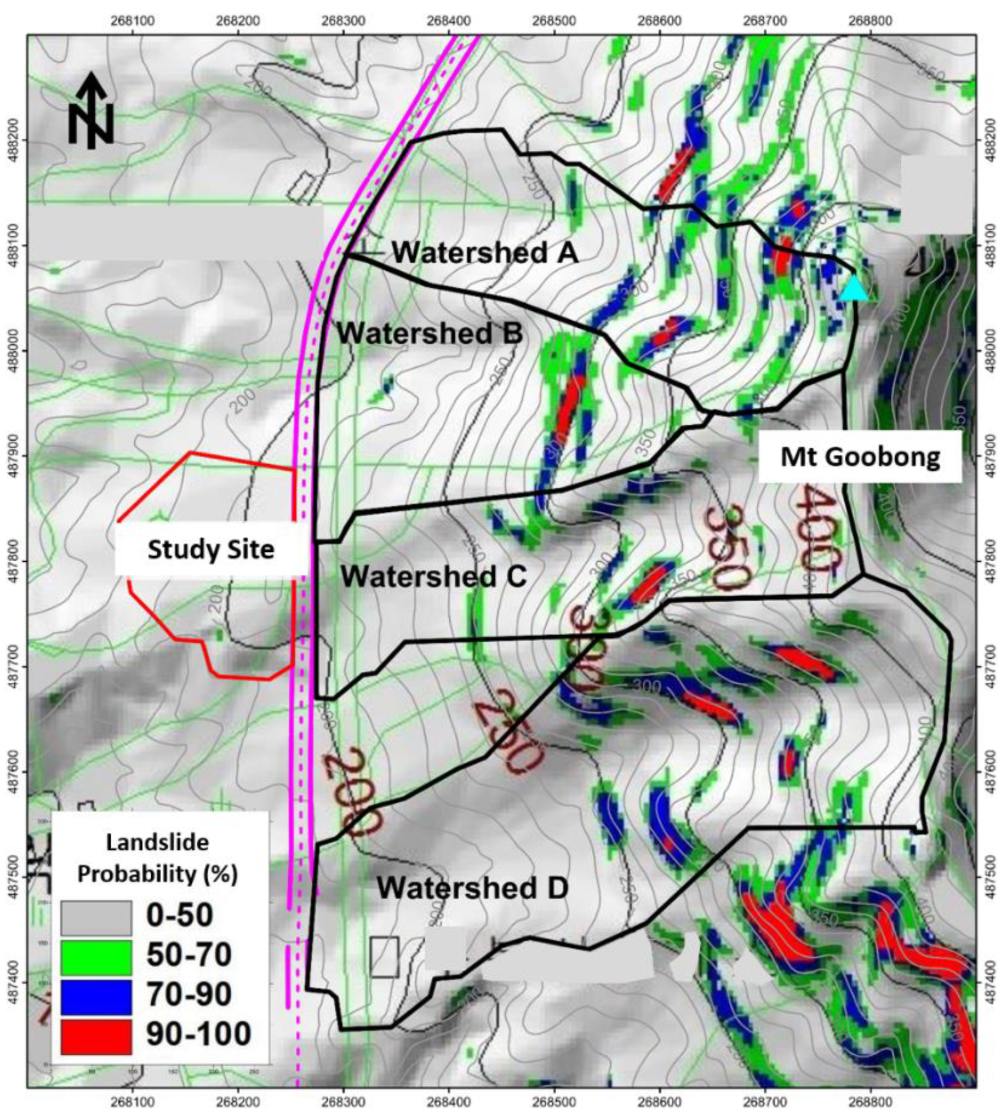
For Debris-2D simulation the mass distribution is necessary as an input factor. The distributions of dry debris were determined according to the area with over 70% of landslide probability (
Figure 7). The thickness of whole mass was set to be 1.5 m uniformly based on the survey results. The mass distributions of dry debris for each watershed are shown in
Figure 8. With the information of dry debris mass, the volume of debris flow was estimated using the concept of equilibrium concentration [
44], i.e., Equation (7). The input factors for Equation (7) are density of debris flow and average slope angle of triggering locations. Based on the measurement results, the density of saturated soil collected from the field was about 1979.6 kg/cm
3.
where
is water density,
is density of dry debris (around 2000 kg/m
3),
is internal friction angle which depends on on-site soil composition (about 37°), and
is average bottom slope angle in the field. The maximum value of
cannot exceed 0.603 [
36].
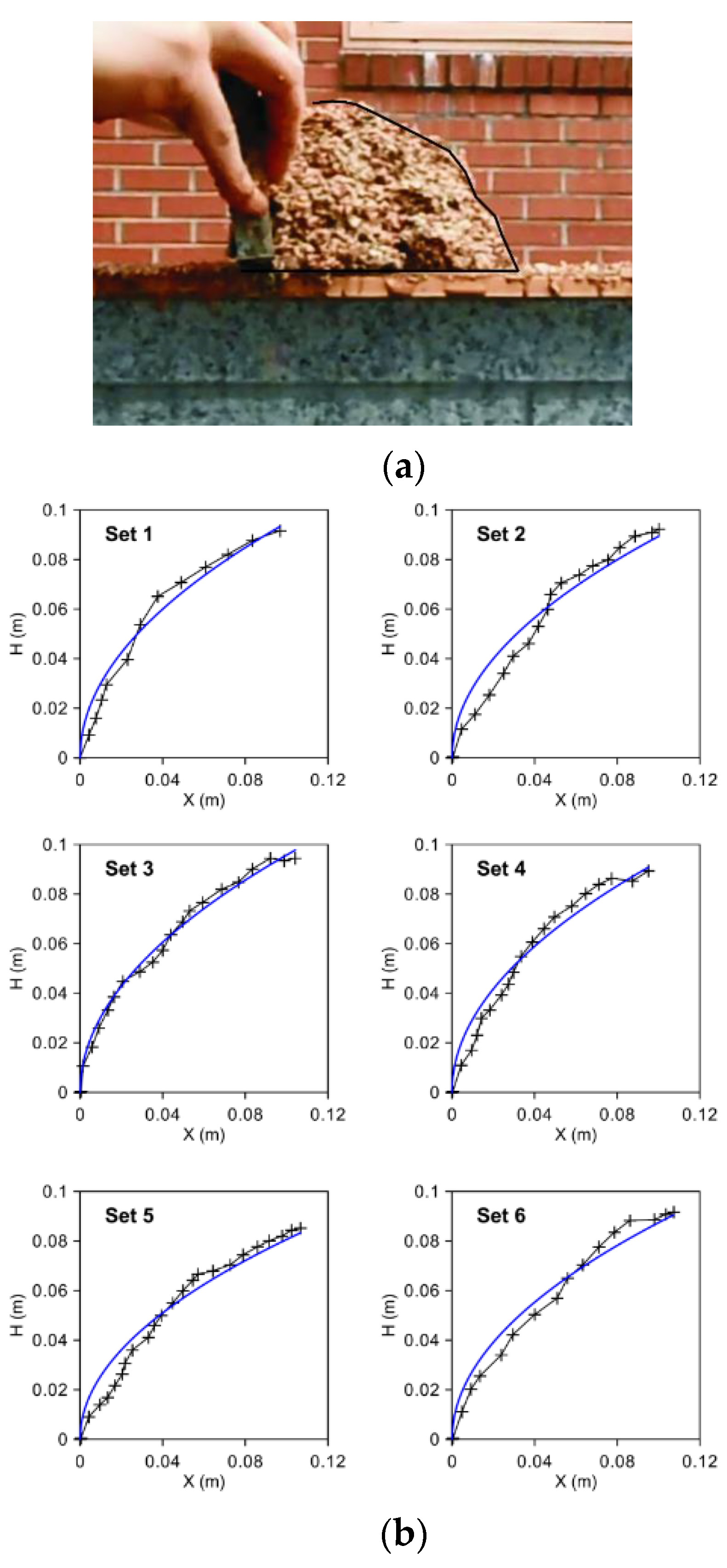
This study conducted six tests for yield stress calibration according to the method (
Figure 7a) by suggested Liu and Hsu [
43]. The test results, shown in
Figure 7b, were used to calculate the value of yield stress with Equation (8) [
43].
where
H denotes the profiles of mass and it depends on longitudinal coordinate
X.
is the yield stress. The value of yield stress was calculated 2800 Pa in this study.
4.2. Results of the Numerical Simulation of Debris Flow
There are four watersheds near the construction site, to the west of Mt Goobong, as shown in
Figure 8. Information on each watershed is listed in
Table 2. In the modeling, it is assumed that the mass of debris-flow at the initiation area comes from a landslide triggered on the slopes. The areas of the landslide and sources of mass used in the simulations were those with a landslide probability over 70%. Based on the regolith mapping, the thickness of loose soil on the slope of Mt Goobong was set to 1.5 m uniformly. On this assumption, the total volume of dry debris across all four watersheds is 24,726.78 m
3 (
Figure 9).
In preparing for damage by the debris flow, it is necessary to consider the worst-case scenario, i.e., when all potential mass becomes debris flow. The worst triggering hazard condition was considered in the simulation. A severe landslide-triggered debris flow occurred in Chooncheon on 27 July 2011 and 15 July 2013. According to Korean Meteorological Agency data, the accumulated rainfall amounts from 26 to 27 July 2011 were 427 mm, and 265 mm from 14 July to 15 July 2013. The simulation used the accumulated rainfall as water input to determine the debris-flow volume. Taking the worst-case scenario, the debris flow was assumed conceptually to involve the entire volume from bottom erosion. However, Liu and Huang [
36] set assumption that the entrained volume of debris flow from bottom erosion is not much compared with total volume of debris flow which is majorly composed of source volume of debris flow. Therefore, Debris-2D considers the initial volume of debris flow as major volume of debris flow to calculate the total volume. The increase of volume by bottom erosion can be included by assigning sufficient initial volume of debris flow. For the simulation, based on the inclined plane test of soil samples collected from the field, the average yield stress was set to 2800 Pa in the saturated condition. This calibrated value of yield stress is typical for a flow mass with a high proportion of coarse sized debris or rock, and therefore high friction, as is shown in
Figure 4,
Figure 5.
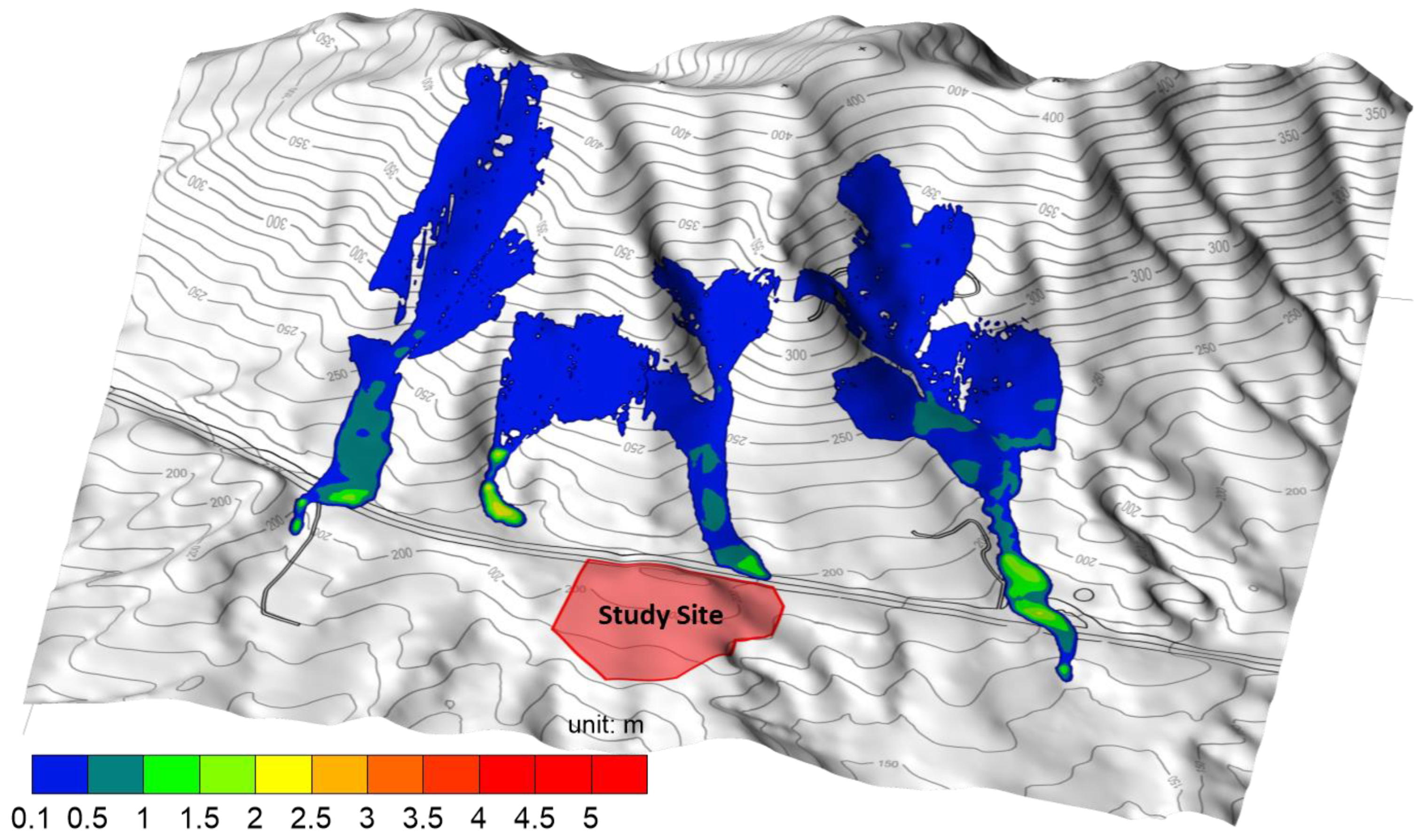
Figure 10 illustrates, in three dimensions, the eventual deposition locations in the four watersheds. The debris in Watersheds A and D flows across Jamboree Road, which is located between Mt Goobong and the site, before deposition. In Watershed B the debris is deposited on the mild slopes before reaching Jamboree Road. However, in Watershed C the final deposition of debris is very close to the southern part of the construction site. Simulated flows and debris thicknesses for each watershed are depicted in
Figure 11,
Figure 12,
Figure 13,
Figure 14 and
Figure 15.
4.2.1. Watershed A
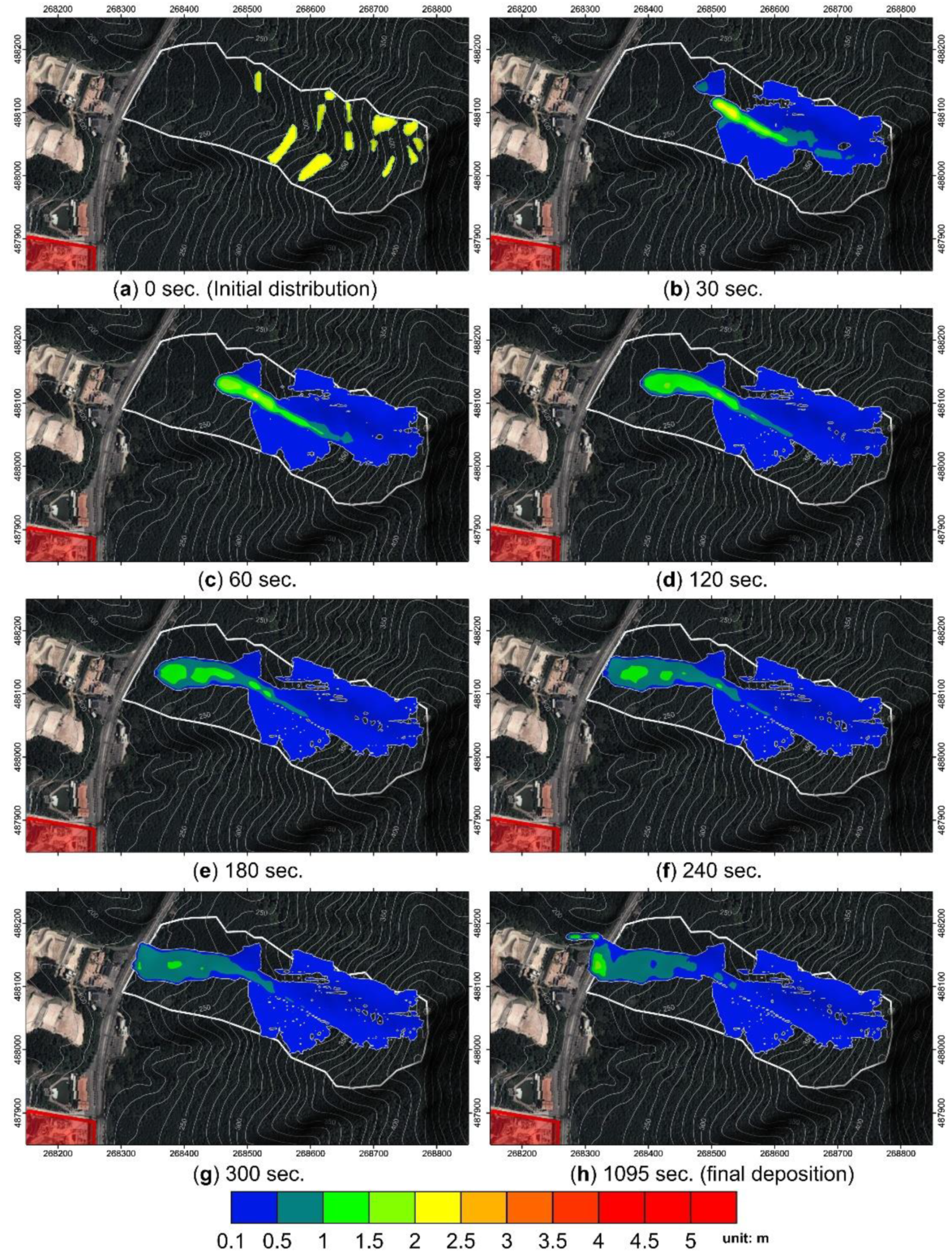
The simulated flow thicknesses, at different times, are shown in
Figure 11. Debris flow stops 1095 s after initiation.
Figure 16a shows the maximum flow speeds over the flow period. From the insert in
Figure 16a the maximum speed was 10.04 m/s at 1.6 s after initiation. At 240 s the debris flow reaches Jamboree Road and begins to slow down and deposit on the road. Then, some of the mass flows down along a small gully and finally stops at 1095 s, as shown in
Figure 11h. The simulation shows that debris flow in Watershed A does not influence the target site. However, debris flow may damage the road, the civilian area along the gully, and the nearby electric power cables.
4.2.2. Watershed B
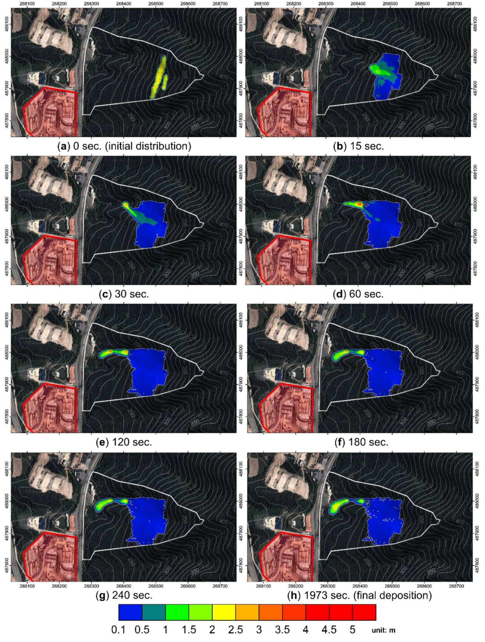
The simulated flow thicknesses, at different times, are shown in
Figure 12. Debris flow stops 1973 s after initiation.
Figure 16b shows the maximum speeds over the flow period. From the insert in
Figure 16b the maximum speed was 6.03 m/s after 6.3 s. Because the topography near the parking lot, which is located at the bottom of Watershed B, slopes gently, the flow speed decreases, and deposition occurs in this area. The final area affected by debris flow (after 1973 s) is shown in
Figure 12h. Because the distance from the final deposition to the target site is around 90 m, the results suggest no direct impact of debris flow on the construction site. However, the possibility of influence on the construction site should be considered if the assessed volume of debris is increased. In that case, debris flow could cause some damage to the road, the civilian area near the parking lot, and the electric power cables in the area.
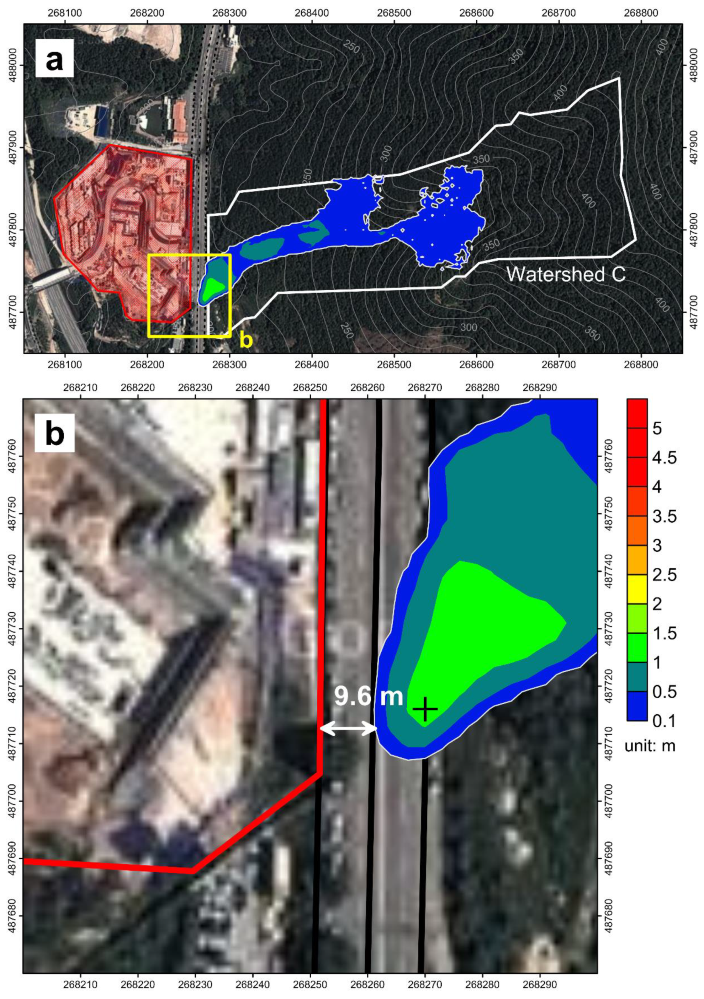
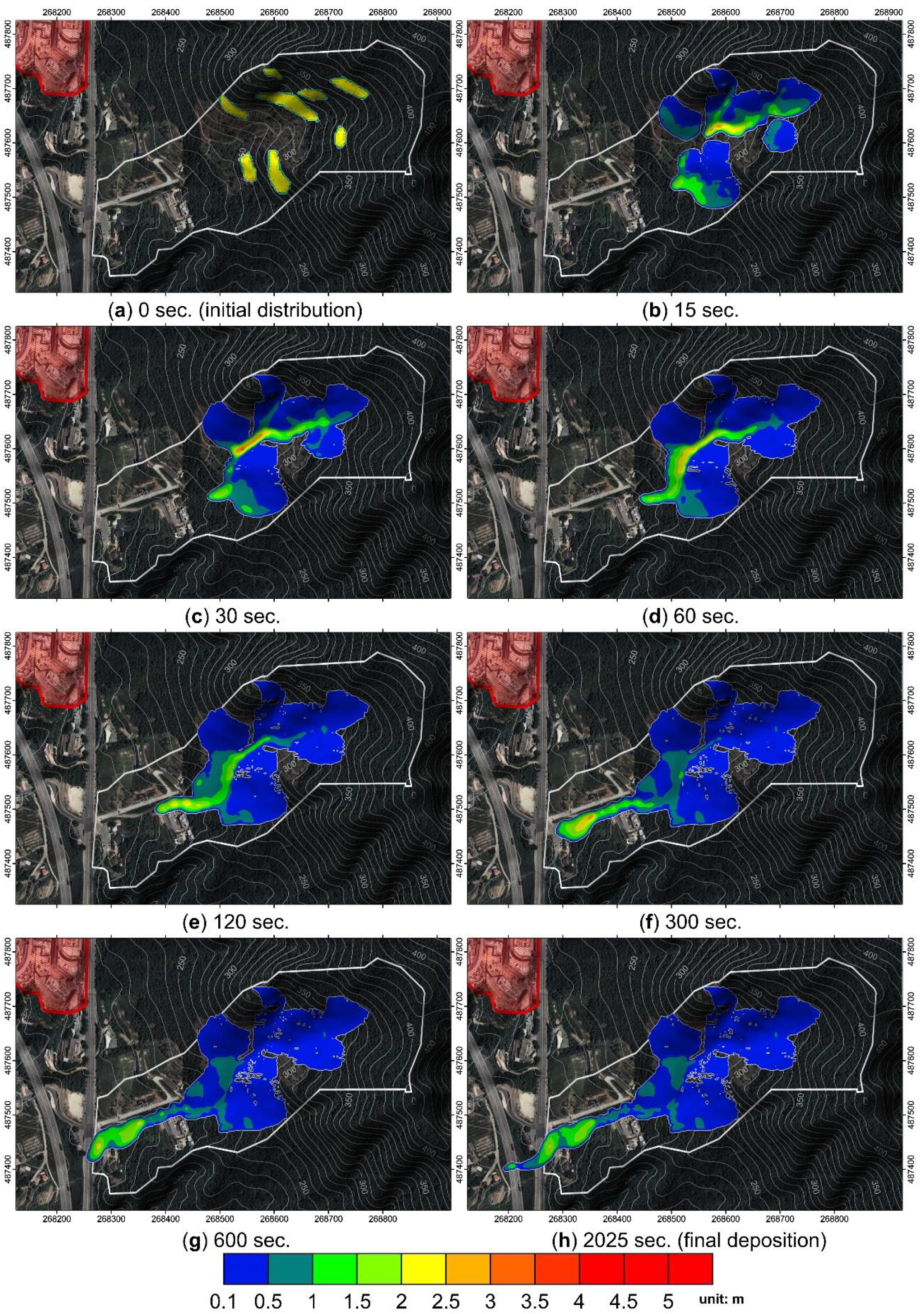
4.2.3. Watershed C
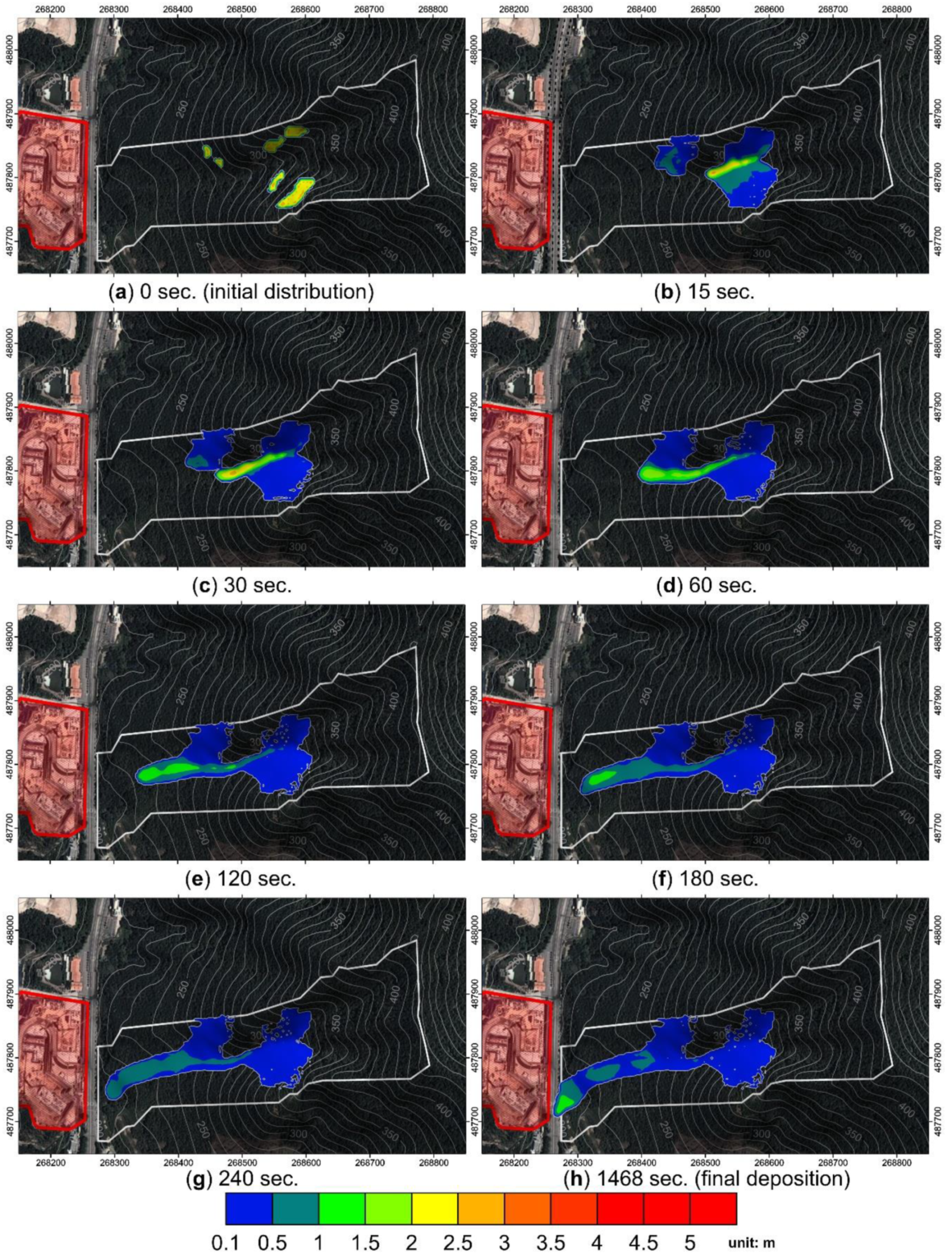
The simulated flow thicknesses, at different times, are shown in
Figure 13. Debris flow stops 1468 s after initiation.
Figure 16c shows the maximum speeds over the flow period. From the insert in
Figure 16c the maximum velocity was 10.82 m/s after 1.1 s. As shown in
Figure 13g, the debris flow approaches Jamboree Road four minutes (240 s) after initiation, and flow speed decreases over the gentler topography. The front of the final deposition is very close to the target site, only 9.6 m (
Figure 14), and the maximum depth of deposition is 1.19 m. Therefore, the construction site has the potential to be impacted by debris flow. Based on this simulation result, appropriate countermeasures should be applied in the area.
4.2.4. Watershed D
The simulated flow thicknesses, at different times, are shown in
Figure 15. Debris flow stops 2025 s after initiation.
Figure 16d shows the maximum speeds over the flow period. From the insert in
Figure 16d the maximum velocity is 10.74 m/s after 2.4 s. At 96 s the debris flow hits a house near the gully with depth more than 2 m, as shown in
Figure 15e. It reaches Jamboree Road after 456 s and starts to deposit on the road. After 2025 s the debris flow stops. In this watershed, the debris flow does not influence the target site. However, the road, and the civilian area, may be damaged by debris flow. In addition, because some electric power cables near the area are likely to be affected by the debris flow, some mitigating countermeasures are needed.
5. Discussion
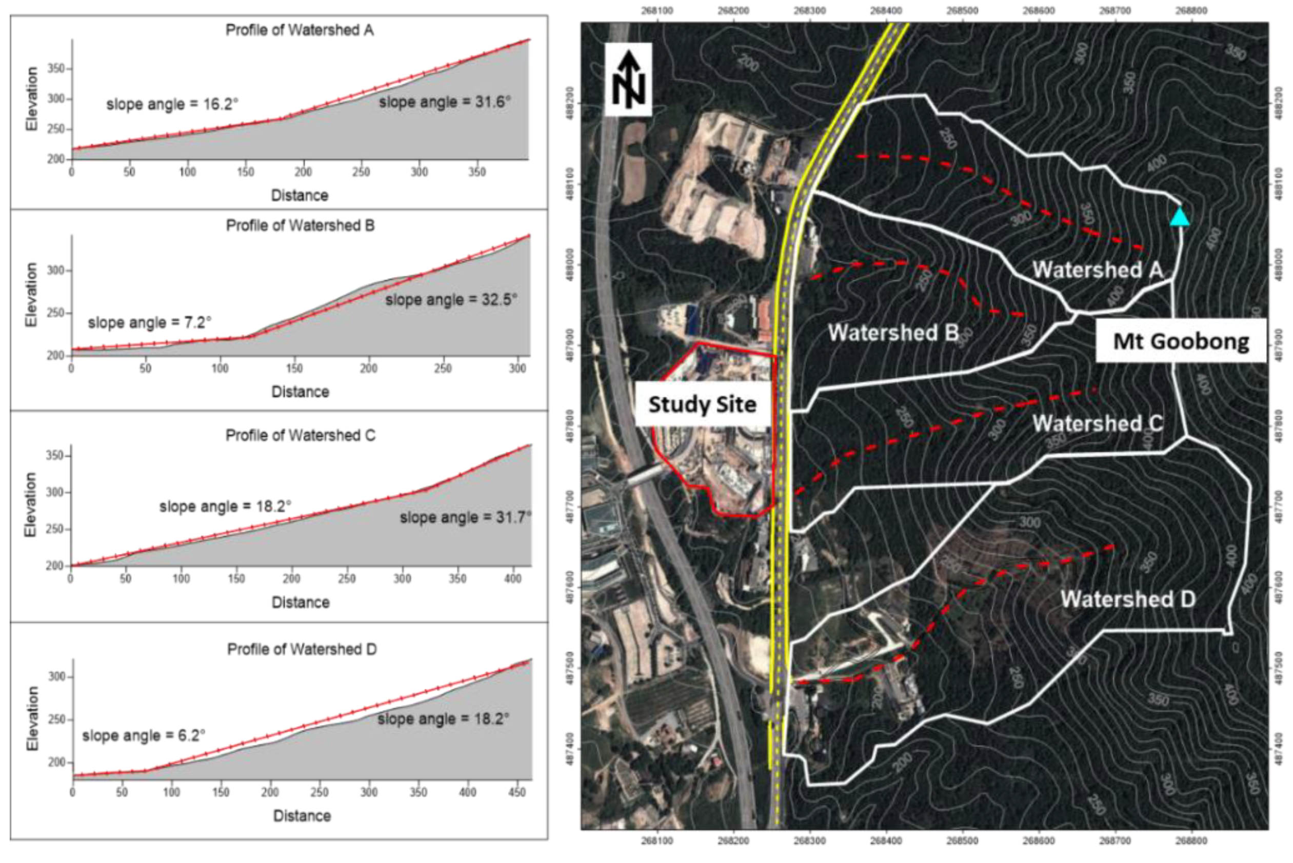
This study used slope angles to simulate debris-flow runout distances. In each of four watersheds, slopes were plotted along the debris-flow direction (
Figure 17). Because each slope section shows just one point of inflection (PI), the simulations used average slopes on either side of the PI. In Watershed A, the PI is located 183 m from the bottom of the slope. The average slope of the lower part is 16.2 degrees and that of the upper part is 31.6 degrees. In Watershed B, which has its PI at 119 m, the average slope of the lower part is 7.2 degrees and that of the upper part is 32.5 degrees. Watershed C has a PI at 322 m with average slopes of 18.2 degrees and 31.7 degrees in the lower and upper parts, respectively. In Watershed D, the PI is at 74 m and the average slopes are 6.2 degrees below the PI and 18.2 degrees above.
The simulations show a debris flow in Watershed C approaching within 9.6 m of the target site. This result reflects the relationship between debris runout distances and slope angles, with Watershed C having steeper average slopes, across both parts, than the other watersheds. The steeper slopes mean that the speed of debris flow does not reduce much until arriving at the bottom of the slope. The debris flow in Watershed C, therefore, came nearer to the target site than in the four watersheds. In the case of Watershed B, the slope below the PI is a very gentle 7.2 degrees while the upper part has the steepest average slope angle in all the watersheds. This would induce fast debris flow on the upper slope, but below the PI the gentle slope area significantly reduces the debris flow speed and the flow energy. Therefore, in Watershed B, the simulated debris flow does not reach the target site even though the debris flow starting point in Watershed B is, among the watersheds, the nearest to the target site. Based on the simulation results, the slope angle is a major factor influencing debris-flow runout distances.
Debris runout distances are determined by several factors, in addition to slope angle, including the volume of debris, quantity of water, physical and rheological properties of the soil. Debris-2D considers the volume of debris and yield stress are significant in calculating runout distance. Liu and Huang [
36] discussed model sensitivity to yield stress and the volume of debris. They explained that the effect of varying volume of debris was three to four times larger than that of varying yield stress in case of Chi-Chi debris flow. As mentioned in
Section 3.2, Liu and Hsu [
43] found that, if yield stress is 100 times larger, the front location of the affected area only reduces by 50 m. However, if the volume of debris flow is just 10 times larger, the front location increases by almost 300 m. The greater influence of debris volume is reflected here in the similar pattern of runout distances among the watersheds. Watersheds C and D which have larger debris volumes, in combination with rainfall water volume, have longer runout distances than the other watersheds (
Table 2). In particular, Watershed D has the largest area and the largest debris-flow volume in the study area. This may explain why the simulation shows the longest runout distance in Watershed D even though the average slope is gentler than in the other watersheds.
The major advantage of the methodology used in this study is that the dynamics of debris flows can be simulated accurately. In addition, initial mass volume and occurrence location were evaluated by integrating the proposed landslide susceptibility model with a mechanically based debris flow model. Therefore, this study has successfully delineated the dangerous zones and affected area of debris flows from multiple watersheds, and it will be considered as an important reference of countermeasure engineering for the construction site. On the other hand, the methodology used in this study is difficult to predict the timing of debris flow occurrence. However, this drawback can be easily overcome by installing monitoring systems to each watershed based on the analysis results. Consequently, the authors believe that the methodology is practical and sustainable for the mitigation of debris flow hazards. This study estimated the yield stress by a simplified laboratory test with soil collected in the field. Because the soil was classified as the same type of residual colluvium, which had been weathered from gneisses, the numerical simulations of debris flow were performed with identical yield stress values in all watersheds. However, the application of watershed specific values of the yield stress would likely generate more accurate simulations of debris flow. For further study, yield stresses should be estimated for the various soils based on in-field regolith mapping and prediction of the saturation characteristics of the soils in each watershed.
6. Conclusions
This study analyzed landslide susceptibility and, based on this, simulated the runout distance of debris flows near a construction site in Korea. Before the landslide susceptibility analysis, and to understand the distribution of soils in the study area, this study mapped the regolith and determined that Mt Goobong is composed primarily of outcrops, residual colluvium, and talus. The outcrops are gneisses and schists which have only limited exposure near the top of the mountain even though the mountain slopes are between 30 and 40 degrees. The residual colluvium is broadly distributed over Mt Goobong with thicknesses of 1.0–1.5 m. These thick colluvia potentially produce high volumes of debris when landslides and debris flows occur in the area. The rock fragments in the valley colluvium is composed of the same materials, such as schists and gneisses pebbles, which are distributed over Mt Goobong.
This study analyzed landslide susceptibility based on a landslide prediction map of the study area which had been drawn in 2008. The landslide prediction used a logistic regression model. In the prediction map, based on 250 mm of rainfall in 24 h, the areas with 70–90% of landslide probability were 3.5% of the analyzed area; those with probability over 90% were 0.79% of the area. Relative to the location of the construction site, the two nearest valleys both have high (over 70%) landslide probability areas. Two additional valleys, to the north and south, also have several areas with over 70% landslide probability.
Based on the landslide susceptibility analysis, numerical simulation of debris flow was performed to assess the likelihood of damage to the construction site by debris flows. According to the simulations, debris flow in Watershed C may approach very near to the boundary of the site. The distance between the front of debris deposition and the construction site was 9.6 m. Therefore, the construction site may be impacted by debris flows in Watershed C. Although the simulation results in Watersheds A and D indicate no direct influence on the construction site, they may damage the road and other facilities at the base of Mt Goobong. The simulations also showed that the debris runout distance is strongly influenced by the on-slope volume of debris in the source area and by the slopes along the debris-flow path.
This study is dealing with the case study that simulated debris runout distance coupled with landslide occurrence prediction in upper mountain areas in order to assess the safety of the construction site. In general, there are limited previous studies which analyze runout distance of debris flow and the possibility of landslide initiation together. For a more reliable simulation of runout distance, landslide information, such as triggering locations and the amount of debris transported from head areas, should be obtained. Therefore, the analysis process proposed in this study improves the reliability of debris runout distances with more accurate information of debris volumes in upper mountain areas. This approach will be effective to secure disaster preparedness in our society.
Author Contributions
Conceptualization and methodology, B.-G.C. and J.C.; formal analysis and software, Y.-H.W. and K.-F.L.; Simulation, J.C., Y.-H.W. and B.-G.C.; investigation, B.-G.C., J.C. and H.-J.P.; writing—original draft preparation, B.-G.C., Y.-H.W., K.-F.L., J.C. and H.-J.P. All authors have read and agreed to the submitted version of the manuscript.
Funding
This research was supported partly by the Basic Research Project (Grant No. 20-3412-1) of the Korea Institute of Geoscience and Mineral Resources (KIGAM) funded by the Ministry of Science and ICT of Korea and partly by the National Research Foundation of Korea (NRF) grant funded by the Korea government (MSIT) (NRF-2019R1F1A1058063). This research was also supported partly by the Korea Environmental Industry and Technology Institute grant funded by the Ministry of Environment (2020002840002).
Conflicts of Interest
The authors declare no conflict of interest. The funders had no role in the design of the study; in the collection, analyses, or interpretation of data; in the writing of the manuscript, or in the decision to publish the results.
References
- Lacasse, S.; Nadim, F. Landslide risk assessment and mitigation. In Landslides—Disaster Risk Reduction; Sassa, K., Canuti, P., Eds.; Springer: Berlin, Germany, 2009; pp. 31–51. [Google Scholar]
- Xie, M.; Esaki, T.; Cai, M. A time-space based approach for mapping rainfall induced shallow landslide hazard. Environ. Geol. 2004, 46, 840–850. [Google Scholar] [CrossRef]
- Salciarini, D.; Godt, J.W.; Savage, W.Z.; Conversini, P.; Baum, R.L.; Michael, J.A. Modeling regional initiation of rainfall-induced shallow landslides in the eastern Umbria Region of central Italy. Landslides 2006, 3, 181–194. [Google Scholar] [CrossRef]
- Godt, J.W.; Baum, R.L.; Savage, W.Z.; Salciarini, D.; Schulz, W.H.; Harp, E.L. Transient deterministic shallow landslide modeling: Requirements for susceptibility and hazard assessments in a GIS framework. Eng. Geol. 2008, 102, 214–226. [Google Scholar] [CrossRef]
- Liu, C.N.; Wu, C.C. Mapping susceptibility of rainfall-triggered shallow landslides using a probabilistic approach. Environ. Geol. 2008, 55, 907–915. [Google Scholar] [CrossRef]
- Fell, R.; Corominas, J.; Bonnard, C.; Cascini, L.; Leroi, E.; Savage, W.Z. Guidelines for landslide susceptibility, hazard and risk zoning for land use planning. Eng. Geol. 2008, 102, 85–98. [Google Scholar] [CrossRef]
- Park, H.J.; Lee, J.H.; Woo, I. Assessment of rainfall-induced shallow landslide susceptibility using a GIS-based probabilistic approach. Eng. Geol. 2013, 161, 1–15. [Google Scholar] [CrossRef]
- Corominas, J.; van Westen, C.; Frattini, P.; Cascini, L.; Malet, J.P.; Fotopoulou, S.; Catani, F.; Van Den Eeckhaut, M.; Mavrouli, O.; Agliardi, F.; et al. Recommendations for the quantitative analysis of landslide risk. Bull. Eng. Geol. Environ. 2014, 73, 209–263. [Google Scholar] [CrossRef]
- Alvioli, M.; Guzzetti, F.; Rossi, M. Scaling properties of rainfall induced landslides predicted by a physically based model. Geomorphology 2014, 213, 38–47. [Google Scholar] [CrossRef]
- Chae, B.-G.; Lee, J.-H.; Park, H.-J.; Choi, J. A method for predicting the factor of safety of an infinite slope based on the depth ratio of the wetting front induced by rainfall infiltration. Nat. Hazards Earth Syst. Sci. 2015, 15, 1835–1849. [Google Scholar] [CrossRef]
- Chae, B.-G.; Cho, Y.C.; Song, Y.S.; Kim, K.S.; Lee, C.O.; Choi, Y.S. Development of Landslide Prediction and Mitigation Technologies; Ministry of Knowledge Economy: Seoul, Korea, 2009; pp. 109–131. [Google Scholar]
- Tsai, T.L.; Tsai, P.Y.; Yang, P.J. Probabilistic modelling of rainfall-induced shallow landslide using a point estimate method. Environ. Earth Sci. 2015, 73, 4109–4117. [Google Scholar] [CrossRef]
- Dietrich, W.E.; Bellugi, D.; De Asua, R.R. Validation of the shallow landslide model, SHALSTAB, for forest management. In Land Use and Watersheds: Human Influence on Hydrology and Geomorphology in Urban and Forest Areas; Wigmosta, M.S., Burges, S.J., Eds.; American Geophysical Union: Washington, DC, USA, 2001; pp. 195–227. [Google Scholar]
- Chae, B.-G.; Kim, W.Y.; Cho, Y.C.; Kim, K.S.; Lee, C.O.; Choi, Y.S. Development of a logistic regression model for probabilistic of debris flow. Korean Soc. Eng. Geol. 2004, 14, 211–240. [Google Scholar]
- Park, H.-J.; West, T.R.; Woo, I. Probabilistic analysis of rock slope stability and random properties of discontinuity parameters, Interstate Highway 40, Western North Carolina, USA. Eng. Geol. 2005, 79, 230–250. [Google Scholar] [CrossRef]
- Zhang, L.L.; Zhang, L.M.; Tang, W.H. Rainfall-induced slope failure considering variability of soil properties. In Risk and Variability in Geotechnical Engineering; Hicks, M.A., Ed.; Thomas Telford Ltd.: London, UK, 2005; pp. 183–188. [Google Scholar]
- Yilmaz, I.; Keskin, I. GIS based statistical and physical approaches to landslide susceptibility mapping (Sebinkarahisar, Turkey). Bull. Eng. Geol. Environ. 2009, 68, 459–471. [Google Scholar] [CrossRef]
- Zhu, H.; Zhang, L.M.; Zhang, L.L.; Zhou, C.B. Two-dimensional probabilistic infiltration analysis with a spatially varying permeability function. Comput. Geotech. 2013, 48, 249–259. [Google Scholar] [CrossRef]
- Rossi, G.; Catani, F.; Leoni, L.; Segoni, S.; Tofani, V. HIRESSS: A physically based slope stability simulator for HPC applications. Nat. Hazards Earth Syst. Sci. 2013, 13, 151–166. [Google Scholar] [CrossRef]
- Ali, A.; Huang, J.; Lyamin, A.V.; Sloan, S.W.; Griffiths, D.V.; Cassidy, M.J.; Li, J.H. Simplified quantitative risk assessment of rainfall-induced landslides modelled by infinite slopes. Eng. Geol. 2014, 179, 102–116. [Google Scholar] [CrossRef]
- Raia, S.; Alvioli, M.; Rossi, M.; Baum, R.L.; Godt, J.W.; Guzzetti, F. Improving predictive power of physically based rainfall-induced shallow landslide models: A probabilistic approach. Geosci. Model Dev. 2014, 7, 495–514. [Google Scholar] [CrossRef]
- Chae, B.-G.; Park, H.-J.; Catani, F.; Simoni, A.; Berti, M. Landslide prediction, monitoring, and early warning: A concise review of state-of-the-art. Geosci. J. 2017, 21, 1033–1070. [Google Scholar] [CrossRef]
- Atkinson, P.M.; Massari, R. Generalized linear modelling of susceptibility to landsliding in the central Apennines, Italy. Comput. Geosci. 1998, 24, 373–385. [Google Scholar] [CrossRef]
- Ohlamacher, G.C.; Davis, J.C. Using multiple logistic regression and GIS technology to predict landslide hazard in northeast Kansas, USA. Eng. Geol. 2003, 69, 331–343. [Google Scholar] [CrossRef]
- Das, I.; Sahoo, S.; van Westen, C.; Stein, A.; Hack, R. Landslide susceptibility assessment using logistic regression and its comparison with a rock mass classification system along a road section in the northern Himalayas (India). Geomorphology 2010, 114, 627–637. [Google Scholar] [CrossRef]
- Suzen, M.L.; Kaya, B.S. Evaluation of environmental parameters in logistic regression models for landslide susceptibility mapping. Int. J. Digit. Earth 2012, 5, 338–355. [Google Scholar] [CrossRef]
- Budimir, M.E.A.; Atkinson, P.M.; Lewis, H.G. A systematic review of landslide probability mapping using logistic regression. Landslides 2015, 12, 419–436. [Google Scholar] [CrossRef]
- Corominas, J. The angle of reach as a mobility index for small and large landslides. Can. Geotech. J. 1996, 33, 260–271. [Google Scholar] [CrossRef]
- Hungr, O.; Evans, S.G.; Bovis, M.; Hutchinson, J.N. Review of the classification of landslides of the flow type. Environ. Eng. Geosci. 2001, 7, 221–238. [Google Scholar] [CrossRef]
- Crosta, G.B.; Cucchiaro, S.; Frattini, P. Validation of semiempirical relationships for the definition of debris-flow behaviour in granular materials. In Proceedings of the 3rd International Conference on Debris-Flow Hazards Mitigation: Mechanics, Prediction and Assessment, Davos, Switzerland, 10–12 September 2003; Rickenmann, D., Chen, C.L., Eds.; Millpress Science Publishers: Rotterdam, The Netherlands, 2003. [Google Scholar]
- Hunter, G.; Fell, R. Travel distance angle for rapid landslides in constructed and natural soil slopes. Can. Geotech. J. 2003, 40, 1123–1141. [Google Scholar] [CrossRef]
- Rickenmann, D. Runout prediction methods. In Debris-Flow Hazards and Related Phenomena; Jakob, M., Hungr, O., Eds.; Springer: Berlin, Germany, 2005; pp. 305–324. [Google Scholar]
- Simoni, A.; Mammoliti, M.; Berti, M. Uncertainty of debris flow mobility relationships and its influence on the prediction of inundated areas. Geomorphology 2011, 132, 249–259. [Google Scholar] [CrossRef]
- Berti, M.; Simoni, A. DFLOWZ: A free program to evaluate the area potentially inundated by a debris flow. Comput. Geosci. 2014, 67, 14–23. [Google Scholar] [CrossRef]
- Reid, M.E.; Coe, J.A.; Brien, D.L. Forecasting inundation from debris flows that grow volumetrically during travel with application to the Oregon Coast Range, USA. Geomorphology 2016, 273, 396–411. [Google Scholar] [CrossRef]
- Liu, K.-F.; Huang, M.C. Numerical simulation of debris flow with application on hazard area mapping. Comput. Geosci. 2006, 10, 221–240. [Google Scholar] [CrossRef]
- Liu, K.-F.; Wu, Y.-H. TXT-tool 3.886-1.1: Debris2D Tutorial. In Landslide Dynamics: ISDR-ICL Landslide Interactive Teaching Tools; Springer: Berlin/Heidelberg, Germany, 2018; pp. 181–189. [Google Scholar]
- Lim, J.S.; Jeong, K.S. Geotechnical Survey Report at NHN Choocheon Campus and IDC Construction Site; S-Tech Consulting Group: Seoul, Korea, 2011; pp. 21–47. [Google Scholar]
- Migon, P. Mass movement and landscape evolution in weathered granite and gneiss terrains. In Weathering as a Predisposing Factor to Slope Movements; Calcaterra, D., Parise, M., Eds.; The Geological Society: London, UK, 2010; pp. 33–45. [Google Scholar]
- Sewell, R.J.; Fletcher, C.J.N. Pilot Study on Regolith Mapping in Hong Kong. GEO Rep. 2000, 1/2000, 45. [Google Scholar]
- Wu, Y.-H.; Liu, K.-F.; Chen, Y.-C. Comparison between FLO-2D and Debris-2D on the application of assessment of granular debris flow hazards with case study. J. Mt. Sci. 2013, 10, 293–304. [Google Scholar] [CrossRef]
- Wu, Y.-H.; Liu, K.-F. Formulas for calibration of rheological parameters of bingham fluid in couette rheometer. J. Fluids Eng. 2015, 137, 041202. [Google Scholar] [CrossRef]
- Liu, K.-F.; Hsu, Y.C. Study on the sensitivity of parameters relating to debris flow spread. Debris Flows: Disasters, Risk, Forecast, Protection. In Proceedings of the International Conference, Pyatigorsk, Russia, 22–29 September 2008; Chernomorets, S.S., Ed.; Sevkavgiprovodkhoz Institute: Pyatigorsk, Russia, 2008. [Google Scholar]
- Takahashi, T. Debris Flow: Mechanics, Prediction and Countermeasures; Taylor & Francis: New York, NY, USA, 2007; p. 448. [Google Scholar]
Figure 1.
Geological map of the study area.
Figure 1.
Geological map of the study area.
Figure 2.
Regolith map in Mt Goobong.
Figure 2.
Regolith map in Mt Goobong.
Figure 3.
Gneiss outcrop near the top of the mountain.
Figure 3.
Gneiss outcrop near the top of the mountain.
Figure 4.
Residual colluvium at Mt Goobong. Size of the red note is 10 × 15 cm. (a) and (b) are in same scale.
Figure 4.
Residual colluvium at Mt Goobong. Size of the red note is 10 × 15 cm. (a) and (b) are in same scale.
Figure 5.
Small scale talus distribution on mountain slopes.
Figure 5.
Small scale talus distribution on mountain slopes.
Figure 6.
Landslide probability map of Mt Goobong (after [
11]).
Figure 6.
Landslide probability map of Mt Goobong (after [
11]).
Figure 7.
(a) Photo of test yield stress calibration. (b) The measured longitudinal profiles and fitting curves (blue line) of 6 sets for calibration of yield stress. (X: longitudinal coordinate, H: height of profile).
Figure 7.
(a) Photo of test yield stress calibration. (b) The measured longitudinal profiles and fitting curves (blue line) of 6 sets for calibration of yield stress. (X: longitudinal coordinate, H: height of profile).
Figure 8.
Distribution of watersheds in the simulation area overlain on the landslide prediction map.
Figure 8.
Distribution of watersheds in the simulation area overlain on the landslide prediction map.
Figure 9.
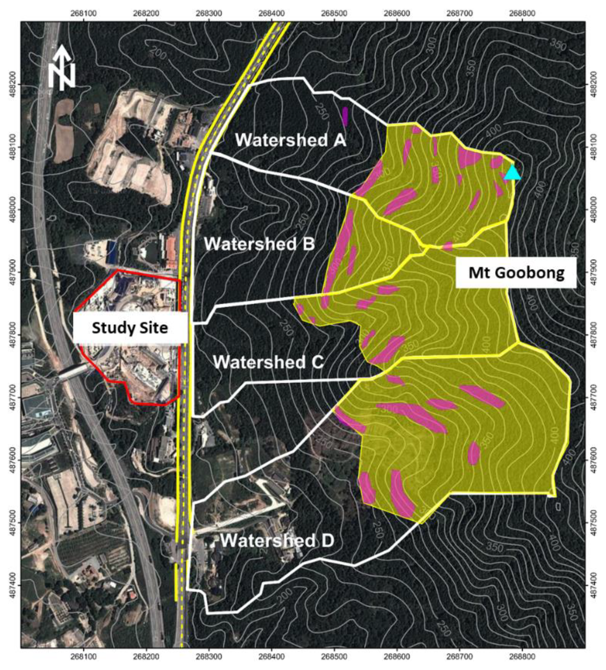
Map of effective rainfall collection areas (yellow) in each watershed. The purple areas denote initial mass distributions and the cyan triangle is the peak of Mt Goobong.
Figure 9.
Map of effective rainfall collection areas (yellow) in each watershed. The purple areas denote initial mass distributions and the cyan triangle is the peak of Mt Goobong.
Figure 10.
Final deposition area of debris in four watersheds. Color scale means thickness of deposited debris.
Figure 10.
Final deposition area of debris in four watersheds. Color scale means thickness of deposited debris.
Figure 11.
Simulated flow and thicknesses of debris at different times (a–h) in Watershed A. (a,h) represent the initial and final (at 1095 s) distributions.
Figure 11.
Simulated flow and thicknesses of debris at different times (a–h) in Watershed A. (a,h) represent the initial and final (at 1095 s) distributions.
Figure 12.
Simulated flow and thickness of debris at different times (a–h) in Watershed B.
Figure 12.
Simulated flow and thickness of debris at different times (a–h) in Watershed B.
Figure 13.
Simulated flow and thickness of debris at different times (a–h) in Watershed C.
Figure 13.
Simulated flow and thickness of debris at different times (a–h) in Watershed C.
Figure 14.
(a) Final deposition of debris in Watershed C. (b) Distance from the front of the final deposition to the site boundary.
Figure 14.
(a) Final deposition of debris in Watershed C. (b) Distance from the front of the final deposition to the site boundary.
Figure 15.
Simulated flow and thickness of debris at different times (a–h) Watershed D.
Figure 15.
Simulated flow and thickness of debris at different times (a–h) Watershed D.
Figure 16.
Simulation of maximum flow speeds over the flow period in each watershed. (a) Watershed A, (b) Watershed B, (c) Watershed C, (d) Watershed D.
Figure 16.
Simulation of maximum flow speeds over the flow period in each watershed. (a) Watershed A, (b) Watershed B, (c) Watershed C, (d) Watershed D.
Figure 17.
Slope profiles for each watershed.
Figure 17.
Slope profiles for each watershed.
Table 1.
Classification of regolith (after [
40]).
Table 1.
Classification of regolith (after [
40]).
| Main Phases | Deposits |
|---|
| Recent Colluvium | Recent landslide debris |
| Depression colluvium |
| Valley colluvium |
| Rock Fall debris (Talus) |
| Relict Colluvium | Relict landslide deposits |
| Residual colluvium |
| Saprolite formation | Saprolite |
Table 2.
Information of watershed area and total volume of debris in each watershed.
Table 2.
Information of watershed area and total volume of debris in each watershed.
| No. | Watershed Area [m2] | Total Dry Debris Volume [m3] | Designed Debris-Flow Volume † [m3] | Area for Collecting Rainfall [m2] | Designed Water Volume by Rainfall Vwater. [m3] | Designed Debris-Flow Volume by Rainfall ‡ [m3] |
|---|
| A | 67,283.35 | 6612.56 | 10,966.11 | 33,778.37 | 5556.54 | 13,996.33 |
| B | 55,942.89 | 3174.32 | 5264.21 | 14,144.71 | 2326.80 | 5860.97 |
| C | 78,296.82 | 3594.74 | 5961.43 | 45,122.06 | 7422.58 | 18,696.67 |
| D | 134,946.30 | 11,345.16 | 18,814.54 | 75,789.91 | 12,467.44 | 31,404.13 |
© 2020 by the authors. Licensee MDPI, Basel, Switzerland. This article is an open access article distributed under the terms and conditions of the Creative Commons Attribution (CC BY) license (http://creativecommons.org/licenses/by/4.0/).


