Abstract
Edge computing is an emerging paradigm that settles some servers on the near-user side and allows some real-time requests from users to be directly returned to the user after being processed by these servers settled on the near-user side. In this paper, we focus on saving the energy of the system to provide an efficient scheduling strategy in edge computing. Our objective is to reduce the power consumption for the providers of the edge nodes while meeting the resources and delay constraints. We propose a two-stage scheduling strategy which includes the scheduling and resource provisioning. In the scheduling stage, we first propose an efficient scheme based on the branch and bound method. In order to reduce complexity, we propose a heuristic algorithm that guarantees users’ deadlines. In the resource provisioning stage, we first approach the problem by virtualizing the edge nodes into master and slave nodes based on the sleep power consumption mode. After that, we propose a scheduling strategy through balancing the resources of virtual nodes that reduce the power consumption and guarantees the user’s delay as well. We use iFogSim to simulate our strategy. The simulation results show that our strategy can effectively reduce the power consumption of the edge system. In the test of idle tasks, the highest energy consumption was 27.9% lower than the original algorithm.
1. Introduction
Traditional cloud computing uses centralized large-capacity cluster devices to process massive amounts of information [1]. All computing processes are centralized in the cloud to facilitate data collection and sharing. This has spawned a series of big data applications. While cloud computing has almost unlimited computing power, to use the cloud computing, it is necessary to bear a lot of communication costs, which inevitably causes the delay. The centralized processing architecture determines that the user’s data needs to be uploaded to the cloud for processing, which makes the delay difficult to reduce. However, with the development of cloud computing, Augmented Reality (AR), Virtual Reality (VR), live video, autopilot, smart medical [2], and other real-time applications of blowout [3,4], the drawbacks of cloud computing have become increasingly prominent. Experiments have shown that edge computing is a good way to handle the application’s latency requirements [5,6]. The edge computing architecture is proposed to solve the problem of large cloud computing delay [7,8,9]. Specifically, edge computing handles tasks that require high latency on the near-user side and puts tasks that could only be processed on the cloud computing platform into the edge server [10,11]. Since the devices on the edge layer are limited power and computing capacities, poor resource allocation for the tasks will result in high latency and power consumption. In this paper, we focus on the reduced power consumption problem in edge computing. This problem is non-trivial mainly due to the following challenges: (i) Since the Internet of Things (IoT) devices generate data constantly, and the analysis must be very rapid [12,13]. One important problem is to find a scheduling strategy of edge devices that can realize the tasks within a lower latency. (ii) Partially battery-powered devices are introduced in the edge-cloud architecture, such as smartphones, laptops, and so on. Thus, the other important problem is to consider the resource allocation for the tasks to reduce the power consumption and realize the endurance of the batteries [14,15].
A preliminary version of this work has been accepted by IEEE INFOCOM 2020 workshop on ICCN [16]. We have included substantial extension over the preliminary version and a summary of differences is included here.
- We first extend our problem into multiple users and propose a two stages scheduling strategy which includes the scheduling and resource provisioning. The published version mainly introduces the resource provisioning stage. While this paper focuses on the scheduling problem between users and edge nodes with energy efficiency. In this paper, we re-formulate the problem and re-define the model. Base on that, we propose two energy-efficient scheduling strategies.
- We propose an efficient scheme based on the branch and bound method for the scheduling stage and discuss the complexity. In this paper, we first propose a scheduling scheme based on the branch and bound method in Algorithm 1, which is a fast search tree algorithm based on a depth-first searching algorithm. Then we discuss the complexity of this algorithm which is . Furthermore, we propose a heuristic algorithm that minimizes the power consumption and guarantees the users’ deadline as well as lower complexity. For Algorithm 1, the time complexity increases exponentially with the expansion of sub-tasks. Thus, we propose a heuristic algorithm in Algorithm 2. The main idea of the algorithm is to select the best node in every layer.
- We conduct various simulations for our scheduling strategy by using the platform we designed. The results are shown from different perspectives to provide conclusions.
In this paper, we focus on saving the power consumption of the system to provide an efficient scheduling strategy in edge computing. Our objective is to reduce the power consumption for multiple users while meeting the resources and delay constraints. Our contributions can be summarized as follows:
- We first implement a normal distribution-based task generation model and add the maximum tolerated delay characteristic of the tasks. We introduce the sleep mode with the lower power consumption for the edge node.
- Based on that, we approach the reduced power consumption problem by virtualizing the edge nodes into master and slave nodes and propose a scheduling strategy through balancing the resources of virtual nodes that reducing the power consumption and guarantees the user’s delay as well.
- We conduct various simulations for our scheduling strategy by using iFogSim. The results are shown from different perspectives to provide conclusions.
The remainder of this paper is organized as follows. Section 2 surveys related works. Section 3 describes the model and then formulates the problem. Section 4 investigates the reduced power consumption problem for users and introduces a scheduling strategy. Section 5 presents the simulations and results. Finally, Section 6 concludes the paper.
| Algorithm 1 Scheduling Scheme based on Branch and Bound Method (SSBB) |
|
| Algorithm 2 Scheduling Scheme based on Backtracking Method (SSBM) |
|
2. Related Work
Edge computing as a new paradigm that used to extend cloud computing to the edge of the network, thus enabling a new breed of applications and services [10]. Nowadays, there are many papers that focus on the power consumption problem in edge computing.
Taneja et al. [17] present a basic module mapping algorithm for efficient utilization of resources in the network infrastructure by efficiently deploying Application Modules in Fog-Cloud Infrastructure for IoT based applications. Barcelo et al. [18] regard energy consumption as the major driver of today’s network and cloud operational costs, and characterize the heterogeneous set of IoT-Cloud network resources according to their associated sensing, computing, transport capacity, and energy efficiency. They mathematically formulate the service distribution problem in IoT-Cloud networks, as a minimum cost mixed-cast flow problem. Zhang et al. [19] study the energy-efficient computation offloading mechanisms in 5G heterogeneous networks for mobile edge computing. They formulate an optimization problem to minimize the energy consumption of the offloading system, where the energy cost of both task computing and file transmission are taken into consideration. Guo et al. [20] consider energy-efficient resource allocation for a multi-user mobile edge computing system which establishes on two computation-efficient models, and they obtain a suboptimal solution with low-complexity by connecting it to a three-stage flow-shop scheduling problem and wisely utilizing Johnson’s algorithm. Huang et al. [21,22] propose a service merging strategy for mapping and co-locating multiple services on devices. They use integer programming to solve this problem in a multi-hop network, use heuristic algorithms to deal with the same problem in a single hop network. These works address the energy-efficient problem using mathematical formulation and propose heuristic algorithms to minimize the energy consumption.
Trinh et al. [23] study the potential of edge computing to address the energy management related applications for limited power-restricted IoT devices while providing low-latency processing of high-resolution visual data. To address the trade-off between processing throughput and energy efficiency, they proposed a smart-driven edge routing based on a sustainable strategy algorithm that uses machine learning. Mavromoustakis et al. [24] propose different methods for implementing edge computing paradigms by using Machine to Machine (M2M) communication in a dense network system with the aim of providing reliability for the delay-sensitive services. Zhang et al. [25] propose a dynamic network virtualization technique to integrate the network resources, and further design a cooperative computation offloading model to achieve high energy-efficiency and reliability in edge computing. Dinh et al. [26] aim to minimize both total tasks’ execution latency and the MD’s energy consumption by jointly optimizing the task allocation decision and the MD’s central process unit (CPU) frequency. They propose an optimization framework of offloading from a single mobile device (MD) to multiple edge devices. Gupta et al. [27] demonstrates the modeling and resource management policies of the IoT environment by using the iFogSim simulator. Besides, they verify the scalability of RAM consumption and execution time simulation tools in different situations. These works address the energy-efficient problem by considering the joint optimization which includes power consumption, latency, and reliability.
However, the above works still have some shortcomings. For example, the scheduling strategy based on machine learning and the addition of new communication links will increase the burden of the edge computing architecture. What’s more, most of these works have only focused on reducing the power consumption, however, they ignored the maximum tolerant delay of the task. These studies all attempt to give an optimal solution on the scheduling algorithm, and the energy-saving function of the edge device itself is not attempted. This paper proposes a new idea to reduce the power consumption of the edge devices based on the scheduling algorithm of device sleep mode. Based on this, the overall power consumption of the system is reduced without increasing the power consumption ratio of the edge device.
3. Model and Problem Formulation
3.1. Network Model
The network model consists of the cloud layer, edge layer, and user layer, which is shown in Figure 1. The communication between the cloud and edge nodes through the gateway and proxy servers. Wireless or wired connections are used between different layers. All notations in this paper are shown in Table 1.
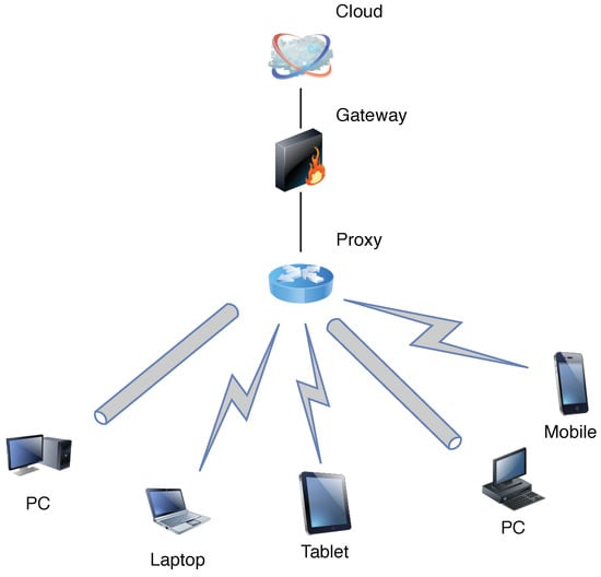
Figure 1.
Edge computing network composition architecture.

Table 1.
Notations.
3.1.1. Edge Layer
In the edge layer, given a substrate distribution of the edge nodes with set , and is the edge node in V. Let denote the computational capability of edge node in cycles per second. For each edge node, we divide one edge node into two virtual nodes, which are the master node and the slave node. and denote the computing capacities of the master and slave nodes, respectively.
3.1.2. User Layer
In the user layer, we use to denote the set of users that connected with edge node j, and denotes the user. The task of device to be processed was defined by a triplet , where denotes the size of the task in bits, and denotes the Million Instructions Per Second (MIPS) of the task. Let denotes the maximum tolerant delay of task i.
In order to ensure the feasibility of our model in a real network, we assume that a set of tasks that arrive at the same time are independent and in line with the normal distribution. Each task evaluates the size of the task by the number of clock cycles it needs to process. Since the scheduling algorithm described in this paper is independent with the amount of the computation of tasks, so we assume that the numbers of clock cycles required to process the tasks are the same. In order to ensure the stability of the experimental results, we use the normal distribution to control the frequency at which tasks are generated. Figure 2 shows the probability of the task we configured. The four lines are the mean parameters of the four normal distributions we set. The horizontal axis is the calculated delay of the next task, and the vertical axis is the possibility of the delay. So, the smaller the mean is, the larger the number of tasks handled. For example, when the value of the mean is 5, the most likely scenario is to wait for 5 clock cycles to generate the next task. With the constraint of this normal distribution probability, both the generation of dynamic tasks and the large deviation of the results will not occur in the process of executing the benchmark multiple times.
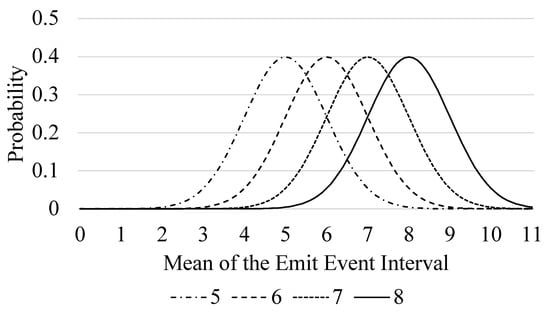
Figure 2.
Probability of the emit interval in different configurations.
3.2. Problem Formulations
In this subsection, we consider minimizing the total energy consumption of users under the latency constraints. Based on this hierarchical structure in Figure 1, users can process the requests either at local devices or remote edge nodes and return the processing results to the user. For user , we use to denote the power consumption for executing task i at local device as shown in Equation (1). is a superlinear function denoting the CPU energy consumption of device i. is a pre-configured model parameter depending on the chip architecture [28,29,30,31].
We use to denote the energy consumption for executing task i at remote edge node as shown in Equation (2).
Let denote the transmit power of device . Let denote the transmission delay which decides by the size of task and the transmission speed . The channel power gain from the device to the edge node can be represented by , where is the path-loss constant, is the reference distance, is the path-loss exponent, and is the distance from device to sensor that it connects. Let denote the channel white Guassian noise, and denote the channel path loss exponent. Hence, the speed of offloaded tasks at edge node is shown in Equation (3).
Let denote the total energy consumption of device , where . In this paper, we formulate the resource provision problem for multiple users in edge computing. Our objective is to find an appropriate scheme for the set of users U that minimizes the total energy consumption and satisfies the constraints on the resources and the maximum tolerant delays. For each device, we use to denote the computation delay, where . Let denote the transmission delay, where . The computation delay on edge node for task i is denoted as , where . Let and denote the processing time and waiting time of on edge node , respectively.
Equations (4) and (5) show the objective of minimizing the total energy consumption for the users. Equation (6) is the constraint on the deadline of the users, which means the total delay can not over the deadline for user i. Equation (7) is the constraint on the computation capacity and the transmit power of each user.
4. Energy-Efficient Scheduling Scheme
In this section, we address the scheduling problem between users and edge nodes with energy efficiency. To solve this problem, we first propose an efficient scheme based on the branch and bound method. Furthermore, we propose a heuristic algorithm that minimizes the power consumption and guarantees the users’ deadline as well as lower complexity.
4.1. Scheduling Scheme Based on Branch and Bound (PSBB)
In this subsection, we propose a scheduling scheme based on the branch and bound method which is a fast search tree algorithm based on a depth-first searching algorithm. According to the problem formulation, we have that the scheduling problem for multiple users can transform into a discrete combinatorial optimization problem. The core idea of our scheduling scheme is efficiently searching candidate solutions on the solution space tree. The candidate solution set is considered to be a rooted tree that forms a complete set on the root. The algorithm explores the branches of the tree, which represents a subset of the solution set. Before enumerating the candidate solutions of a branch, the candidate solution of the branch will be checked according to the feasibility of the current optimal solution based on the estimated upper and lower bounds of the optimal solution. If it cannot produce a better solution than the optimal one currently, the algorithm will discard the solution. The branch and bound method can be applied to a variety of maximum and minimum problems. The above problem happens to be the minimum problem that will solve finite candidate solutions, which meets the requirements of the branch and bound method. For example, if it is assumed that a task needs to be scheduled, the task has a sub-task set . Since each sub-task can be offloaded independently, each sub-task need to be determined the computing location through an algorithm. Therefore, the algorithm in this section needs to build a tree to represent the solution space of the computing location of the sub-task. The layer of the tree represents the possible calculation position of the sub-task n, and each node has 3 children, which are the possible calculation locations for sub-tasks. It is inferred from this that the output (scheduling scheme) is the path from the root to a leaf of this tree. In this algorithm, the solution space is represented as a topology G, as one of the input parameters. The specific steps of applying this algorithm to the above problem are shown in Algorithm 1.
We take the topology of fog nodes G, and the set of users U as our inputs. The output is the scheduling scheme X for the set of users U. We use and to denote the numbers of edge nodes and users, respectively. We first initialize the bound L and temporary set S in lines 3 and 5. In line 6, we calculate the power consumption of sub-tasks, where is the power consumption of sub-task for executing at local device. is the power consumption of sub-task for executing at remote edge node. We send the results into set S and find the minimum one as the branch as shown in lines 7 to 8. Then we calculate the total power consumption for sub-task in line 9. If both and satisfy the constraints, we will check whether is the last sub-task of . If , we will update the bound . Otherwise, we continue to calculate next sub-task in line 15. If either or are beyond the constraints, we will cut this branch and do not continue to traverse in line 18. The entire process ends after all edge nodes are traversed or all sub-tasks of users are finished. We calculate the total power consumption E and return X in lines 23 to 25. The key of this algorithm is to save the optimal solution boundary L as the basis for pruning. Since the power consumption of each node in the searching tree is greater than the power consumption of its parent, when a node’s power consumption exceeds the optimal solution boundary L, it must be concluded that the power consumption of the node and its children must be greater than the current optimal solution boundary. Pruning on this basis, skip the traversal process of the child nodes under this node, so as to achieve the purpose of speeding up the search.
During the running of the algorithm, if all nodes cannot be pruned, the algorithm needs to traverse all branches, which is the worst running condition of the algorithm. We can conclude that, according to the change in the number of model nodes, each additional sub-task adds triple solutions, the complexity of the algorithm is .
4.2. Scheduling Scheme Based on Backtracking Method (SSBM)
For the Algorithm 1, the time complexity increases exponentially with the expansion of sub-tasks, which can be reduced by some heuristic. In this subsection, we propose a heuristic algorithm that minimizes the power consumption and guarantees the users’ deadline as well as lower complexity.
The main idea of the algorithm is to select the best node in every layer. Generally, it seems that the composition of the global optimal solution is not necessarily optimal in every part of the solution. May be multiple sub-optimal solutions forming the global optimal solution. However, with the perspective of reducing complexity, this algorithm significantly reduces the complexity (reducing the exponential level to the linear level), and it is very suitable for scenarios that require the low complexity of the algorithm.
As shown in Algorithm 2, the input and output are the same as Algorithm 1. The first two steps of the algorithm are also completely consistent with Algorithm 1. We perform the same operations as Algorithm 1 lines 5 and 6, in line 3 and 4.The algorithm sorts the calculation results of tasks performed by different nodes by power consumption and selects the set of data with the lowest power consumption in line 5. It is determined whether the cumulative delay sum is less than the maximum tolerable delay of the task in line 6. If it is less than the value, then the power consumption value is recorded as the power consumption set S of the current sub-task in line 7. Otherwise, execute line 10 of the algorithm, that is, delete the solution in the topology tree, and then jump to step 5 to re-select the smallest value. By analogy, the feasible solution and the node path that can realize the power consumption value are output after traversing a feasible solution for the first time. The worst time complexity of SSBM is .
5. Resource Provisioning Strategy
In this section, we introduce a scheduling strategy based on the master-slave model. As the result shown in Figure 3, the master-slave model reduces the power consumption obviously, and also brings more devices able to be scheduled. An inefficient scheduling strategy will lead to the edge nodes cannot effectively participate in the calculation, and produce a huge increase in the task delay. Thus, the main idea of our strategy is triggering the sleep mode of the slave devices as much as possible to reduce the power consumption of the edge nodes, and trying to load balance the resource as much as possible to ensure low latency.
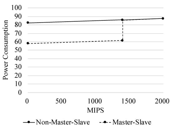
Figure 3.
Power consumption of the device in different configurations.
5.1. Edge Node Virtualization Model
For each edge node, we suppose that there are two different modes that are active and sleep. We use P to denote the power of one edge node, which includes two modes, active mode and sleep mode . Active mode is a high power mode of one edge node. Only the device in the active state can execute the task, and the task scheduling activity is also a kind of activity, which needs the support of the active state. The power consumption under the active mode is linear depending on the CPU usage, i.e., , where b is the power of the edge node under the idle and k is a coefficient that fits the power curve of the edge node. Sleep mode is a very low power mode of one edge node. A device under this mode typically only reserves power for memory and related devices that can be used to wake up. Commonly used wake-up devices are a network card, mouse, keyboard, power button, and so on. Because sleep power is processor-independent, sleep power is the same on all three platforms. In general, the power consumption of the sleep state is extremely low. For a normal PC, this power consumption is about W [32]. In this paper, we use this parameter to simulate the power consumption during sleep.
We used three different edge devices. We regard Config 1 as an original device. In order to reduce the power consumption of the edge nodes, we split the original device into two devices, Configs 2 and 3. To ensure fairness, we guarantee that the sum of MIPS of Configs 2 and 3 is equal to Config 1. We refer to a device combination with only one Config 1 configuration as a non-master-slave, and each has a combination of Configs 2 and 3 called master-slave. We set the master device to Config 2 and the slave device to Config 3. The master device is used to task scheduling and execution, and the slave device only executes tasks and goes to sleep when idles. The subsequent experimental part will be based on this configuration. The specific experimental steps and results can refer to Section 6. Figure 3 is the power consumption value of the edge node under two different strategies, where the horizontal axis is the occupancy rate of the edge node and the vertical axis is the instantaneous power consumption of the node. Figure 3 shows that the power consumption of the combination of master-slave is much lower than the non-master-slave when it is less than 1400 MIPS. This is because the device of Config 2 is running and the device of Config 3 is in the sleep state. In master-slave, devices that do not receive a task can go to sleep when the task that needs to be calculated is none. A device that is in a sleep state can be woken up by other devices through a network command. In a non-master-slave, the device cannot enter the sleep state because there is only one device in the node. The detailed configuration of the simulator is shown in Table 2.
Table 2.
Simulation parameters.
5.2. Resource Provisioning Strategy
As shown in Algorithm 3, we use , , , , , and T as the inputs. and are the numbers of running tasks on the master and slave devices, respectively. and are the capacities of the master and slave devices, respectively. is the MIPS of the target task. T is the maximum tolerated time of the target task. In addition, the rest main notations throughout Algorithm 3 are listed in Table 3. The output is the scheduling strategy for the tasks. We first consider the status of the edge node. If the number of tasks running on the edge node is , it means that there is no task received at this time. Then, we add this task into the master node and check the feasibility in lines 3 to 5. We calculate the remaining computation delay for the task and compare this value to the maximum tolerant time. If it does not exceed, we send the task to the master node. Otherwise, we calculate whether the maximum tolerated delay of the task is exceeded after adding the task to the slave node in lines 6 to 9. If neither of the nodes is satisfied, the task will be sent to the cloud in line 10. If the number of tasks running on the edge node is not 0 when a task arrives, we calculate the relative idleness of the master and slave devices in line 12. We define the value of the relative idleness is determined by the ratio of the master and slave device’s computing capacity to the number of running tasks, where . Then we start to place tasks by considering the relative idleness in lines 13 to 34. If the value is not greater than , it indicates that the slave device is relatively idle at this time. We prioritize place the task on the slave device to calculate the remaining computation delay and compare this value with the maximum tolerated time in line 13. If it is not exceeded, the task will send to the slave device in line 16. Otherwise, we calculate the maximum tolerated delay under the master device in line 18. Similarly, if the remaining computation delay is smaller than the maximum tolerated delay, we send the task to the master device in line 20. Otherwise, we upload the task to the cloud in line 22. If the value is greater than , we change the order of calculation in lines 24 to 34. We calculate the remaining computation delay for the master device first in line 24. If it does not exceed the maximum tolerated delay, we send the task to the master device in line 26. Otherwise, we do the same calculation on the slave device in line 28. If none of the above are satisfied, we send the task to the cloud in line 32.
| Algorithm 3 Resource Provisioning Strategy |
|
Table 3.
Notations.
The functions we used in Algorithm 3 are shown in lines 27 to 39. We calculate task delay after adding the scheduled task to the device in lines 31 to 39. We first add the computing capacity and the max tolerate delay required form the scheduled task to the device in lines 32 to 33, and increase the number of the running tasks by 1 in line 34. We update the computation delays for the tasks on the device, where . Then, we compare whether they exceeded their maximum tolerated delay in line 36. If any of the tasks exceed its maximum tolerated delay, the function will return false which indicates that the task cannot be added into the device. Otherwise, the function returns true. We use two functions to encapsulate the respective calculation parameters of the master and slave devices in lines 27 to 30.
6. Simulation and Results
6.1. Simulation for the Energy-Efficient Scheduling Schemes
In order to check the effectiveness of the energy-efficient scheduling schemes propose in this paper, we built a simulator based on the power and delay model described above. In addition, we have also implemented the following two algorithms as algorithm benchmarks for comparative analysis. (i) Greedy Algorithm without Backtracking (GAB): This algorithm differs from the task scheduling algorithm based on the greedy algorithm described above in that it does not judge the maximum tolerable delay in line 7 and directly enters line 8, so that the first solution is found greedily. While the solution may exceed the maximum tolerable delay. In order to compare the algorithms more fairly, in the subsequent simulation experiments, if the solution obtained exceeds the maximum tolerable delay, the solution will be multiplied by a factor, increasing the power consumption value of the solution. (ii) Greedy Algorithm with Minimum Delay without Backtracking (GAMDB): the difference between this algorithm and the previous algorithm is that the selection of the greedy algorithm, it will be sorted according to the length of the delay, and the solution with the smallest delay is selected each time, in order to expect to find the solution with the smallest delay, as a comparison group of experiments. The network architecture in the simulation is that every 5 user devices access an edge node, there are 5 edge nodes in total, and all edge nodes access one cloud node in common.
In our simulation, the parameters shown in Table 4 which are set for simulation. We pre-configure the coefficient of each edge node in Equation (1) to be 10. What’s more, we define a penalty coefficient which is 630. It denotes the penalty that exceeding the maximum tolerance. The above four algorithms are implemented separately and compared under the same parameters. We run each of the above algorithms 5000 times and average these results. When the averages are stable, record them as follows.
Table 4.
Simulation parameters.
As shown in Figure 4, we implement four algorithms (SSBB, SSBM, GAB, and GAMDB) on our simulator. According to the performance of the above algorithm in the simulator, the following conclusions can be drawn. The optimal solution solved by the SSBB has an absolute advantage among the four algorithms. The SSBM algorithm with backtracking effectively finds the sub-optimal solution. When the task transmission size is small, the gap between the optimal solution and the sub-optimal solution is larger, the maximum gap is 8%. With the increasing size of task transmission, the gap is gradually narrowing, eventually less than 1.8%. Because in the process of traversing the solution space, the first feasible solution found using the greedy algorithm may not be the optimal solution, and the branch and bound method is to subtract the impossible branch under the premise of traversing the entire solution space and found the global optimal solution. Since the algorithm GAB uses more edge-cloud nodes and calculates the transmission power consumption. It has a different slope compared with the first two algorithms. Generally, the power consumption of the local calculation is far greater than the transmission power consumption. This leads to a much smaller fluctuation in the results of this algorithm than other algorithms that use local calculations. Generally, the GAB and GAMDB using the delay to sort are still more power-intensive than other algorithms. Because a penalty coefficient is designed for solutions that use a delay that exceeds the maximum tolerance. For scenarios with low quality of service, these two algorithms can be used to reduce the complexity of the algorithm.
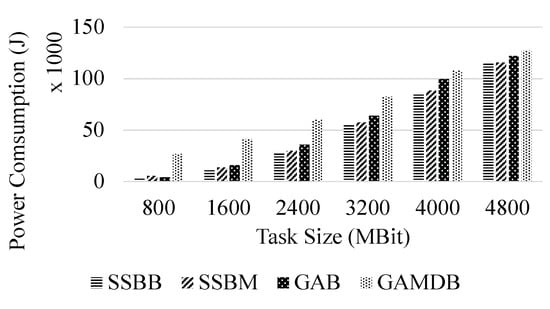
Figure 4.
Total power consumption of the users.
Figure 5 shows the delay of the four algorithms. Except for the GAB algorithm, they all come together and make little difference. However, this is not the case. The value of the solution space is discontinuous under this simulation parameter, and the gap is huge. Because we averaged the obtained data after 5000 executions of the solution obtained. The delays of the solutions of SSBB and greedy are at the boundary of the maximum tolerable delay because they use as more local calculations as possible. The longer the execution time corresponds to the lower the execution power, indicating that these algorithms make full use of task tolerance delay, which is as expected. The solution of GAB uses too much offload computing, resulting in a delay much higher than other algorithms. The delay of the solution obtained by GAMDB is at a low level, because it uses too many local calculations, resulting in very high power consumption.

Figure 5.
Total delay of the users.
6.2. Simulation for the Resource Provisioning Strategy
In this section, we conduct our experiments on the iFogSim simulator platform [27]. iFogSim is a popular simulator in the area of edge computing which implements many features of the edge architecture, such as the edge network structure, the placement of task modules, and the task system. In our simulation, we realize our scheduling strategy and modify the power consumption model to adapt the sleep power consumption mode based on the iFogSim simulator. We assume that each sensor is equipped with a set of edge nodes for receiving tasks. In our simulation, 24 edge nodes are used which divided into 4 groups. The detailed configuration of the simulator is shown in Table 4. For each group, we set six edge nodes that connect to the upper-level cloud through a gateway and a proxy server.
We first performed the scheduling strategy under the master-slave mode and non-master-slave mode. The experimental result is shown in Figure 6. The abscissa is the name of the device under a gateway in the architecture, and the ordinate is the power consumption of the edge nodes in this experiment. According to the result, we find that the power consumption has a certain fluctuation due to the normal distribution, but the mean value is still very stable which means that the power consumption of each node is similar. Thus, we have that the total number of tasks that the edge nodes process is similar which is not affected by the dynamic generation.
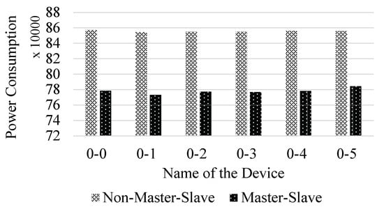
Figure 6.
Power consumption of five edge nodes in a gateway.
As shown in Figure 7, we experiment with different mission generation densities. The horizontal axis is the value of the mean in the normal distribution for each task, and the vertical axis is the total power consumption of the edge nodes in this experiment. The experimental results show that with a mean of 5, the power consumption of the non-master-slave is 3.3% lower than that of the master-slave. In the experiment with a mean of 6, the power consumption dropped by 18.5%. In the experiment with a mean of 7, the power consumption dropped by 26.3%. In the experiment with a mean of 8, the power consumption dropped by 27.9%. It can be concluded that with the intensive task generation, the advantages of the strategy under the master-slave mode are getting smaller and smaller. The algorithm proposed in this paper has obvious optimization of the power consumption when the task density is small. When the task density is large, the power consumption under both modes is nearly the same. As shown in Figure 8, we calculate the delay of two scenarios under different task volumes. The horizontal axis is the value of the mean in a normal distribution for each task, and the vertical axis is the mean of all task delays in this experiment. The experimental results show that in the experiment with a mean of 5, the delay of non-master-slave is 0.04% higher than the delay of master-slave. In the experiment with the means of 6 and 7, the delays increased by 5.25% and 16.69%, respectively. Similarly, the delay increased by 17.07% with a mean of 8. The algorithm proposed in this paper has certain side effects on delay, but in different groups of experiments, the power consumption savings ratio is greater than the delay increase ratio.
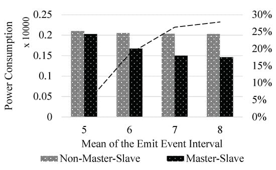
Figure 7.
Total power consumption of the edge nodes.
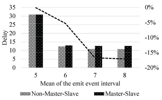
Figure 8.
Total delay of the tasks.
According to the experimental results above, we make the following conjectures. Assuming that a task is a minimum migration unit, we cannot place a task on two devices in parallel. Since the task is indivisible, in the case where the total computing power of the master-slave mode and the non-master-slave mode is the same. When there is no task to be processed, we can see that the power consumption under the master-slave mode is much lower than the non-master-slave mode. When there is only one task to be processed, the slave node must be in a sleep mode under the master-slave mode. The computing capacity under the non-master-slave mode is significantly stronger than the master-slave mode. Thus, there will be a certain increase in the delay under this scenario. When the number of tasks is larger than one, since the capacities of the edge nodes are limited, the performance gap between these two modes is not obvious.
7. Conclusions
In this paper, we focus on reducing the power consumption in edge computing by considering the resources and delay constraints. We propose a two-stage scheduling strategy. In the scheduling stage, we introduce an algorithm based on branch and bound. Base on that, we propose a heuristic algorithm that guarantees users’ deadlines to reduce complexity. In the resource provisioning stage, we approach the problem by virtualizing the edge nodes into master and slave nodes based on the sleep power consumption mode. Then, we propose a scheduling strategy through balancing the resources of virtual nodes that reduce the power consumption and guarantee the user’s delay as well. Extended trace-driven simulations on iFogSim prove the correctness and efficiency of our strategy.
Author Contributions
Conceptualization, J.F. and Y.C.; methodology, Y.C. and S.L.; software, Y.C.; validation, J.F. and S.L.; investigation, J.F., Y.C. and S.L.; resources, J.F.; data curation, Y.C. and S.L.; writing—original draft preparation, Y.C.; writing—review and editing, S.L. and J.F.; visualization, Y.C.; supervision, J.F.; project administration, J.F.; funding acquisition, J.F. All authors have read and agreed to the published version of the manuscript.
Funding
This research is supported by the National Natural Science Foundation of China (61202076), and supported by Beijing Natural Science Foundation (4192007), along with other government sponsors.
Acknowledgments
The authors would like to thank the reviewers for their efforts and for providing helpful suggestions that have led to several important improvements in our work. We would also like to thank all teachers and students in our laboratory for helpful discussions.
Conflicts of Interest
The funders had no role in the design of the study; in the collection, analyses, or interpretation of data; in the writing of the manuscript, or in the decision to publish the results.
References
- Li, J.; Huang, L.; Zhou, Y.; He, S.; Ming, Z. Computation partitioning for mobile cloud computing in a big data environment. IEEE Trans. Ind. Inform. 2017, 13, 2009–2018. [Google Scholar] [CrossRef]
- Alnoman, A.; Anpalagan, A. Towards the fulfillment of 5G network requirements: Technologies and challenges. Telecommun. Syst. 2017, 65, 101–116. [Google Scholar] [CrossRef]
- Goethals, T.; De Turck, F.; Volckaert, B. Near real-time optimization of fog service placement for responsive edge computing. J. Cloud Comput. 2020, 9, 1–17. [Google Scholar] [CrossRef]
- Ha, K.; Chen, Z.; Hu, W.; Richter, W.; Pillai, P.; Satyanarayanan, M. Towards wearable cognitive assistance. In Proceedings of the 12th Annual International Conference on Mobile Systems, Applications, and Services; ACM: New York, NY, USA, 2014; pp. 68–81. [Google Scholar]
- Premsankar, G.; Di Francesco, M.; Taleb, T. Edge computing for the Internet of Things: A case study. IEEE Internet Things J. 2018, 5, 1275–1284. [Google Scholar] [CrossRef]
- Zhang, K.; Cao, J.; Liu, H.; Maharjan, S.; Zhang, Y. Deep reinforcement learning for social-aware edge computing and caching in urban informatics. IEEE Trans. Ind. Inform. 2019, 16, 5467–5477. [Google Scholar] [CrossRef]
- Ren, J.; Guo, H.; Xu, C.; Zhang, Y. Serving at the edge: A scalable IoT architecture based on transparent computing. IEEE Netw. 2017, 31, 96–105. [Google Scholar] [CrossRef]
- Brogi, A.; Forti, S. QoS-aware deployment of IoT applications through the fog. IEEE Internet Things J. 2017, 4, 1185–1192. [Google Scholar] [CrossRef]
- Xiao, S.; Liu, C.; Li, K.; Li, K. System delay optimization for Mobile Edge Computing. Future Gener. Comput. Syst. 2020, 109, 17–28. [Google Scholar] [CrossRef]
- Shi, W.; Cao, J.; Zhang, Q.; Li, Y.; Xu, L. Edge computing: Vision and challenges. IEEE Internet Things J. 2016, 3, 637–646. [Google Scholar] [CrossRef]
- Hussain, B.; Du, Q.; Imran, A.; Imran, M.A. Artificial Intelligence-powered Mobile Edge Computing-based Anomaly Detection in Cellular Networks. IEEE Trans. Ind. Inform. 2019, 16, 4986–4996. [Google Scholar] [CrossRef]
- Zhang, T.; Xu, Y.; Loo, J.; Yang, D.; Xiao, L. Joint computation and communication design for UAV-assisted mobile edge computing in IoT. IEEE Trans. Ind. Inform. 2019, 16, 5505–5516. [Google Scholar] [CrossRef]
- Wang, T.; Wang, P.; Cai, S.; Ma, Y.; Liu, A.; Xie, M. A unified trustworthy environment establishment based on edge computing in industrial IoT. IEEE Trans. Ind. Inform. 2019, 16, 6083–6091. [Google Scholar] [CrossRef]
- Ahn, J.; Lee, J.; Yoon, S.; Choi, J.K. A novel resolution and power control scheme for energy-efficient mobile augmented reality applications in mobile edge computing. IEEE Wirel. Commun. Lett. 2019, 9, 750–754. [Google Scholar] [CrossRef]
- Gu, X.; Ji, C.; Zhang, G. Energy-Optimal Latency-Constrained Application Offloading in Mobile-Edge Computing. Sensors 2020, 20, 3064. [Google Scholar] [CrossRef]
- Fang, J.; Chen, Y.; Lu, S. A Scheduling Strategy for Reduced Power Consumption in Mobile Edge Computing. In Proceedings of the IEEE INFOCOM 2020-IEEE Conference on Computer Communications Workshops (INFOCOM WKSHPS), Toronto, ON, Canada, 6–9 July 2020; pp. 1190–1195. [Google Scholar]
- Taneja, M.; Davy, A. Resource aware placement of IoT application modules in Fog-Cloud Computing Paradigm. In Proceedings of the 2017 IFIP/IEEE Symposium on Integrated Network and Service Management (IM), Lisbon, Portugal, 8–12 May 2017; pp. 1222–1228. [Google Scholar]
- Barcelo, M.; Correa, A.; Llorca, J.; Tulino, A.M.; Vicario, J.L.; Morell, A. IoT-cloud service optimization in next generation smart environments. IEEE J. Sel. Areas Commun. 2016, 34, 4077–4090. [Google Scholar] [CrossRef]
- Zhang, K.; Mao, Y.; Leng, S.; Zhao, Q.; Li, L.; Peng, X.; Pan, L.; Maharjan, S.; Zhang, Y. Energy-Efficient Offloading for Mobile Edge Computing in 5G Heterogeneous Networks. IEEE Access 2016, 4, 5896–5907. [Google Scholar] [CrossRef]
- Guo, J.; Song, Z.; Cui, Y.; Liu, Z.; Ji, Y. Energy-Efficient Resource Allocation for Multi-User Mobile Edge Computing. In Proceedings of the GLOBECOM 2017—2017 IEEE Global Communications Conference, Singapore, 4–8 December 2018. [Google Scholar]
- Huang, Z.; Lin, K.J.; Yu, S.Y.; Hsu, J.Y.J. Co-locating services in IoT systems to minimize the communication energy cost. J. Innov. Digit. Ecosyst. 2014, 1, 47–57. [Google Scholar] [CrossRef]
- Huang, Z.; Lin, K.J.; Yu, S.Y.; Hsu, J.Y.J. Building energy efficient internet of things by co-locating services to minimize communication. In Proceedings of the 6th International Conference on Management of Emergent Digital EcoSystems, Buraidah Al Qassim, Saudi Arabia, 15–17 September 2014; pp. 101–108. [Google Scholar]
- Trinh, H.; Calyam, P.; Chemodanov, D.; Yao, S.; Lei, Q.; Gao, F.; Palaniappan, K. Energy-aware mobile edge computing and routing for low-latency visual data processing. IEEE Trans. Multimed. 2018, 20, 2562–2577. [Google Scholar] [CrossRef]
- Mavromoustakis, C.X.; Batalla, J.M.; Mastorakis, G.; Markakis, E.; Pallis, E. Socially Oriented Edge Computing for Energy Awareness in IoT Architectures. IEEE Commun. Mag. 2018, 56, 139–145. [Google Scholar] [CrossRef]
- Zhang, Z.; Zhang, W.; Tseng, F.H. Satellite mobile edge computing: Improving QoS of high-speed satellite-terrestrial networks using edge computing techniques. IEEE Netw. 2019, 33, 70–76. [Google Scholar] [CrossRef]
- Dinh, T.Q.; Tang, J.; La, Q.D.; Quek, T.Q. Offloading in mobile edge computing: Task allocation and computational frequency scaling. IEEE Trans. Commun. 2017, 65, 3571–3584. [Google Scholar]
- Gupta, H.; Vahid Dastjerdi, A.; Ghosh, S.K.; Buyya, R. iFogSim: A toolkit for modeling and simulation of resource management techniques in the Internet of Things, Edge and Fog computing environments. Softw. Pract. Exp. 2017, 47, 1275–1296. [Google Scholar] [CrossRef]
- Chen, X. Decentralized Computation Offloading Game for Mobile Cloud Computing. IEEE Trans. Parallel Distrib. Syst. 2015, 26, 974–983. [Google Scholar] [CrossRef]
- Chen, X.; Jiao, L.; Li, W.; Fu, X. Efficient Multi-User Computation Offloading for Mobile-Edge Cloud Computing. IEEE/ACM Trans. Netw. 2016, 24, 2795–2808. [Google Scholar] [CrossRef]
- Lin, X.; Wang, Y.; Xie, Q.; Pedram, M. Task Scheduling with Dynamic Voltage and Frequency Scaling for Energy Minimization in the Mobile Cloud Computing Environment. IEEE Trans. Serv. Comput. 2015, 8, 175–186. [Google Scholar] [CrossRef]
- Lyu, X.; Tian, H.; Ni, W.; Zhang, Y.; Zhang, P.; Liu, R.P. Energy-Efficient Admission of Delay-Sensitive Tasks for Mobile Edge Computing. IEEE Trans. Commun. 2018, 66, 2603–2616. [Google Scholar] [CrossRef]
- Mao, Y.; Zhang, J.; Song, S.; Letaief, K.B. Power-delay tradeoff in multi-user mobile-edge computing systems. In Proceedings of the 2016 IEEE Global Communications Conference (GLOBECOM), Washington, DC, USA, 4–8 December 2016; pp. 1–6. [Google Scholar]


© 2020 by the authors. Licensee MDPI, Basel, Switzerland. This article is an open access article distributed under the terms and conditions of the Creative Commons Attribution (CC BY) license (http://creativecommons.org/licenses/by/4.0/).