1. Introduction
The efficiency and profitability of photovoltaic (PV) plants are highly controlled by their operation and maintenance (O&M) procedures. For example, an 18MWp plant with the availability of 99% (1% caused by uncontrolled failures) can cause economic losses up to 156K euros per year [
1]. The malfunctions of a PV system are typically detected only if a significant reduction in energy production has been observed, while the time until the damage is determined can last up to a year [
2]. Thus, a reduction of up to 18.9% of the annual energy production can be caused due to undetected faults in a PV system [
3], which significantly affects the financial efficiency of the PV installation. The energy production of PV modules is degraded by faults, such as hot spots, cracks, or deposition of dirt, among others [
4]. Additionally, the Potential Induced Degradation of solar cells may also reduce their energy production by up to 30% after a few years of operation. Overall, the faults of PV modules comprise up to 73.5% a PV plant malfunctions [
5]. Thus, early and reliable detection of faults is a key aspect for the monitoring of PV plants and their effective operation during their lifetime period.
Today, the effective diagnosis of any possible fault of PV plants remains a technical and economic challenge, especially when dealing with large-scale PV plants. At present, PV plant monitoring is carried out using one of the following approaches: (a) electrical performance measurements and (b) image processing techniques. The first approach presents limited fault detection capabilities, it is both costly and time-consuming. Additionally, it is incapable of fast identification of the physical location of the fault. In the same way, Infrared Thermography (IRT) imaging has been used for the characterization of PV module failures. IRT imaging provides a real-time two-dimensional image of PV module from which temperature distribution of the module surface can be assessed [
6,
7,
8]. Hence, IRT imaging is a valuable non-destructive inspection technology to identify, classify, and locate PV modules operating with defects. The identification and classification are based on temperature anomalies present on the surface of PV module. However, the setup and processing are rather complex for manual IRT imaging analysis and an experienced human operator is required.
Unmanned Aerial Vehicles (UAVs) for IRT imaging of PV plants for health status monitoring of PV modules have been identified as a cost-effective approach that offers 10-–15 fold lower inspection times than conventional techniques [
9]. However, the implementation of a cost-effective method to scan and check huge PV plants represents major challenges, such as the cost and time of detecting PV module defects with their classification and exact localization within the solar plant [
10]. Moreover, many technological considerations should be taken into account for a proper inspection of photovoltaic plants [
11].
This work provides a fully automated approach for the: (a) detection, (b) classification, and (c) geopositioning of the thermal defects in the PV modules. The system has been tested on a real PV plant in Spain. The obtained results indicate that an autonomous solution can be implemented for a full characterization of the thermal defects. The main contribution of this work is the proposal of a comprehensive procedure for automated thermal image analysis. This procedure addresses from image pre-processing (e.g., image undistortion), the detection and classification of the defects, to the final location of the thermal defects. Moreover, this procedure also considers the best practices and conditions for image acquisition. Finally, the contribution also addresses several procedures to make the processing procedure as robust as possible (e.g., the detection of the panels surface in order to filter the thermal defects, or a quality indicator that checks if the individual panels detection was correctly performed, among others). The robustness of the panel detection procedure is also a major contribution that distinguishes this work from previous methods. A novel method that is based on image reprojection and function minimization is developed to detect the panels from the images. The proposed approach is based on a combination of adaptive thresholding and the correction of perspective distortion by considering the panel corner. Minimizing the distance from the reprojection on multiple adjacent panels ensures correct panel detection, regardless of orientation or camera position. This robust approach is verified in extensive tests.
The rest of this work is organized, as follows. In
Section 2, the main steps for image undistortion are summarized. Image undistortion is a key point when pre-processing the thermal images, because it can give a better representation of all of the elements captured by the thermal camera without optical aberrations. Aerial IRT considerations for PV applications are summarized in
Section 3. This Section is complemented with
Section 4, where the acquisition procedure to collect all of the thermal images is carried out. The automated image processing procedure is explained in
Section 5, which consists of several algorithms to properly cope with the processing of the thermal images.
Section 6 summarizes the main results when evaluating the proposed algorithm with the database. Finally, the conclusions are given in
Section 7.
2. Image Undistortion
The projection of points in the scene onto images is usually described by a series of geometric transformations using the pinhole model [
12]. First, the world coordinates in the scene are transformed to camera coordinates while using a three-dimensional (3D) rigid-body transformation that involves three rotations (
) and three translations (
). These parameters are often referred to as extrinsic parameters. The transformation can be expressed as (
1), where
and
represent the coordinates of points in world and camera coordinates, and
are the coefficients of the rotation matrix using the angles
,
, and
.
Points in camera coordinates are transformed next to pixel coordinates using a combination of perspective projection and 2D affine transformation. These transformations are usually combined in a single form as (
2), where
are the column and row of the pixel,
f is the focal distance,
and
are the size of the pixels, and
and
are the translation coefficients that compensate for displacements of the central pixel. These parameters are often referred to as intrinsic parameters.
This linear model is not accurate, as it does not take lens distortions into account [
13]. Lens imperfections produce non-linear projections of the scene points onto the image plane.
Figure 1 shows the effects of the most common lens distortions.
An additional transformation is required to compensate for these optical distortions. The most common distortion model is the polynomial model [
14]. Other models also exist, such as the division model [
15]. In general, eight coefficients are considered, six to model the radial distortion and two to model the tangential distortion. However, the last five radial distortion coefficients are only used for severe distortion, such as in wide-angle lenses. Radial distortion is related to light rays bending near the edges of the lens. Tangential distortion is related to nonalignment issues between the image plane and the lens. Distortion is usually modeled as (
3) and (
4), where
denote the distorted points,
,
are the radial distortion coefficients, and
are the tangential distortion coefficients. These radial and tangential distortion coefficients are part of the intrinsic parameters, as they do not depend on the scene viewed.
Lens distortions provoke different irregular patterns and undesirable artifacts in the image, such as curvatures of lines. Straight lines in the scene do not remain straight in the projected image, provoking difficulties in image processing and interpretation. Therefore, image undistortion is a recommended pre-processing step for further image analysis [
16]. Image undistortion is performed by applying image interpolation with a reverse distortion. This is a non-trivial problem with no analytical solution due to the non-linearity of the distortion model. Generally, iterative solvers are used. Image undistortion requires an accurate camera calibration in order to estimate the intrinsic camera parameters. Subsequently, lens distortion can be removed by applying the reverse distortion model, eliminating image artifacts due to lens aberrations.
Many different methods are available to perform camera calibration [
17]. The most common are based on calibration patterns printed on flat plates [
18], particularly using the procedure proposed in [
19]. This method requires different observations of the pattern with different orientations. Control points on the pattern with well-known correspondences to world coordinates and extracted. The set of correspondences between the image and world coordinates are used to first estimate linear projection models for each orientation. Subsequently, intrinsic camera parameters are calculated considering all orientations. Finally, a non-linear optimization method is used to finely tune the camera parameters, including distortion.
Calibration plates are readily available for most camera configurations. However, cameras that are installed on aerial vehicles usually have long focal lengths that limit the applicability of printed calibration patterns due to the required size of the pattern. In this work, an alternative approach is proposed: camera calibration that is based on natural landmarks. The landmarks are situated on a flat surface on the scene, and they are observed while the aerial vehicle moves around them while the camera rotates. Multiple images are acquired from the same natural landmarks with different orientations as a result. Therefore, they can be assimilated to images acquired from a calibration pattern on a flat plate, and the procedure proposed in [
19] can be used to calibrate the camera and estimate the distortion parameters. Moreover, the same procedure can be used for visible and infrared cameras, depending on the selected natural landmarks. Landmarks must be distinguishable in visible images, but also in infrared images, i.e, they are required to emit different infrared radiation than the surroundings in the scene. This can be achieved when using materials of different emissivity [
20]. The proposed approach in this work as natural landmarks are the corner of windows. Windows are placed on flat walls, i.e., all control points (corners) lie on the same plane. Moreover, glass and window frames have very different emissivity than walls. Thus, they can be easily distinguished in the infrared spectrum. The proposed approach has a major advantage when compared with other methods: no complex calibration apparatus is needed. Moreover, there is no need to establish artificial landmarks. The result is a straightforward method that provides a reliable estimation of the camera parameters, both for visible or for infrared cameras. These parameters can then be used to undistort the acquired images.
Figure 2 shows the results of image undistortion for visible images. Different images are acquired from the facade of a building with windows. For each image, natural landmarks on the corner of some windows are labeled. The positions of the windows on the facade are well-known. Thus, correspondences between image and world coordinates can be established, which is the required information for camera calibration. The estimated camera parameters can then be used to undistort the images, as can be seen in
Figure 2c,d. The resulting images do not present the undesirable artifacts that are caused by lens distortion: straight lines in the scene do remain straight in the images, as can be seen in the figure.
The same approach can be used with infrared images.
Figure 3 shows the equivalent images in the infrared spectrum. The same procedure is followed: corners in the images are associated with the positions in the scene and the camera is calibrated. The images are undistorted using the estimation of lens distortion. In this case, the differences between the original images and the undistorted are less noticeable, as the lenses in the infrared camera have less aberration than the lenses in the visible camera.
3. Aerial Infrared Thermography for Photovoltaic Applications
IRT can be used for the detection of a great number of defects in PV cells, modules, and strings, since the majority of the defects have an impact on their thermal behavior. Such thermal patterns have been identified and classified in previous studies (e.g., [
21,
22]) and they are now standardized in the international norm IEC TS 62446-3 Edition 1.0 2017-06. In this sense, the most common IR image patterns can be seen in
Figure 4. The IR patterns can be classified into two groups. In the first group (represented by the upper part of the image), the defects correspond to both a module or one row (sub-string) warmer than the others. On the other hand, the second group (represented by the lower part of the image) is in connection with single cells that are warmer than the others.
Therefore, the objective of a IRT inspection is to detect and classify these defects in the thermal images. Traditionally, IRT inspections for PV applications are performed with handheld IR cameras on the ground or on lifting platforms to increase the coverage. This procedure is dependent on human labor and competence and very time-consuming and labor-intensive. As a result, the monitoring accuracy is prone to human error and the uncertainty of the method increased. IRT can be combined with aerial technologies, like UAV, in order to increase the cost-effectiveness and employ IRT for large-scale PV plants or roof-mounted PV systems with limited access. Furthermore, and in connection again with the international norm IEC TS 62446-3, some considerations, which are briefly commented, as follows, should be taken into account when acquiring the thermal images in photovoltaic IR inspections. First of all, The IR-camera image shall be taken as perpendicular to the PV module surface as possible avoiding reflections from the drone. In cases where the image cannot be taken perpendicular to the PV module surface the angle between the camera and the PV module plane should still be greater than 30° to minimize the effects of reflected background. Moreover, fast camera carriers (e.g., aerial drones) can cause a negative effect on the image quality, as the typically used bolometer detectors have a long time constant and high camera movement velocities above 3 m/s [
23] may cause smearing. In connection with the environmental conditions, the recommended values are: (a) a minimum irradiance value of 600 W/m
in the plane of the PV module is necessary, (b) a maximum wind speed of 28 km/h, (c) clear sky, (d) and no soiling (cleaning is recommended, e.g., if bird droppings exist). Finally, the GSD should have a maximum value of 3 cm/pixel. Standard c-Si PV panels have a cell of 15 × 15 cm (see
Figure 5).
Therefore, norm IEC TS 62446-3 recommends that all PV modules should be recorded with a minimum resolution of 5 × 5 pixels per cell. However, this resolution seems to be not enough to properly register all of the thermal defects when performing aerial inspections of photovoltaic plants. More specifically, in [
24], the authors proved that the GSD strongly influenced the ability to detect the thermal defects. They considered that GSD of 1.8 should be necessary to properly detect all thermal defects. Finally, one last consideration when analyzing thermal defects is in connection when categorizing the severity of a thermal defect, which is not included in the norm IEC TS 62446-3. One common approach is to define ranges of temperature attending the severity of the anomalies [
24], being performed by TSK PV plant operators, which use this classification criterion in their thermography reports. Differences higher than 30 °C are considered as severe failures, from 10 °C to 30 °C are considered as medium severity failures and lower than 10 °C as minor failures. In
Figure 6, three hotspots can be seen, but only two of them can be considered as severe failures.
In conclusion, all of these considerations should be taken into account when performing aerial thermographic inspections of photovoltaic plants.
4. Database and Acquisition Procedure
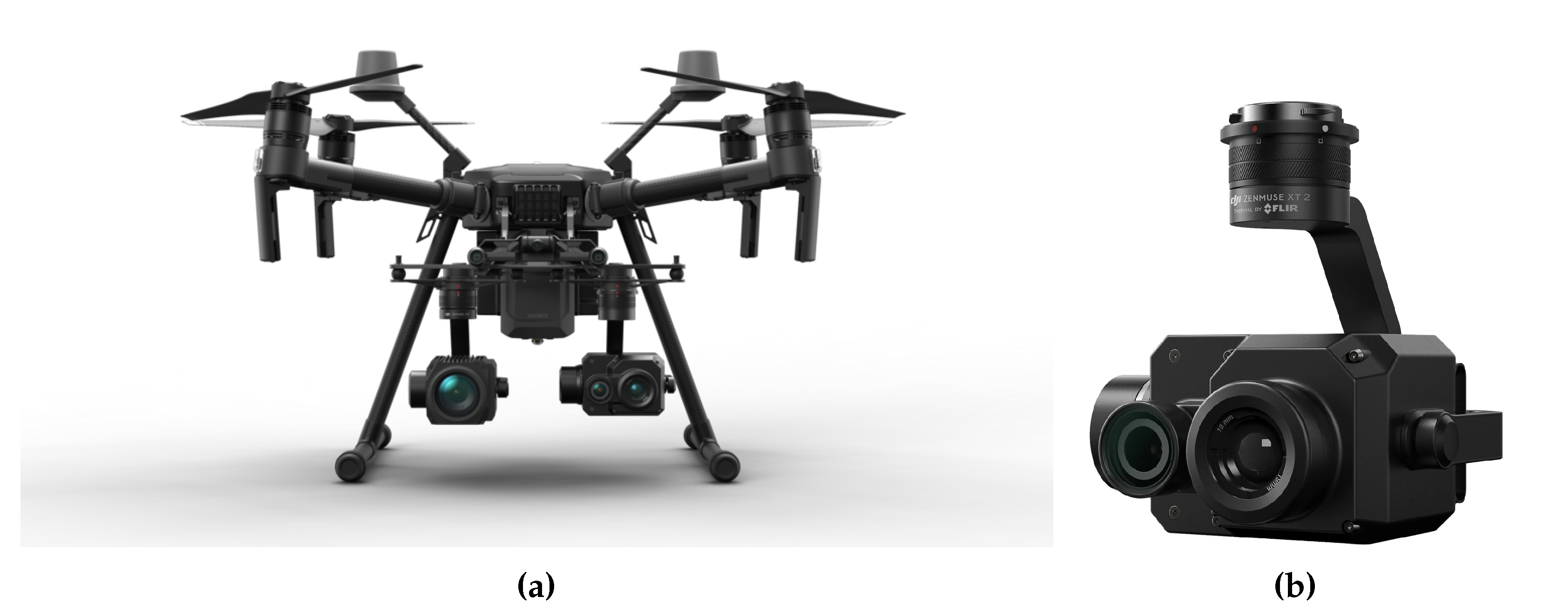
All if the images were automatically collected by a drone over a photovoltaic plant. In connection with the drone, the DJI Matrice 210 RTK V2 was used, which can be seen in
Figure 7a.
As can be seen, there are two cameras attached to the aircraft. The camera on the left is the DJI Zenmuse Z30 (not used in the acquisition process). The camera on the right is the DJI Zenmuse XT2. This camera, which can be seen in
Figure 7b enlarged, integrates a high-resolution FLIR thermal sensor and a 4K visual camera with DJI’s stabilization. Therefore, both a thermal and a visual (RGB-Red-Green-Blue) image are recorded by the XT2 camera. Under the scope of this publication, only the thermal image is used and, hence, the RGB image is not used for the detection of defects in the photovoltaic panels. The RGB image is only used for visualization purposes. The XT2 can be mounted with different lens models: 9 mm, 13 mm, 19 mm, and 25 mm. In this case, the selected lens model is the one offering 25 mm. These models provide a 25° × 20° Field Of View (FOV) angle with 0.680 mrad.
In connection with the thermal camera, an uncooled VOx Microbolometer sensor is used, providing a resolution of 640 × 512 pixels. The sensor also provides a 17 m pixel pitch size and the spectral band is in the range of 7.5–13.5 m. The thermal camera can be configured in the range of −25° to 135 °C (High Gain) or in the range of −40° to 550 °C (Low Gain). In this case, the camera was configured in the first range with a High Gain.
In
Figure 8, some key points in connection with the acquisition process are shown. The photovoltaic plant is located in the province of León, Spain. This plant has a size of 1.56 hectares.
In
Figure 8 left, it can be seen that the DJI mission planner estimated a total of 298 photos, but a total of 321 images was finally acquired.
Figure 8 right shows the GPS position associated with each image. All of the images were acquired with a relative altitude of (approximately) 25 m. The exact relative altitude associated with each image is stored using the Exchangeable Image File Format (EXIF) [
25]. In this sense, all of the necessary information that will be used in the processing procedure is stored using this image file format. As an example, in
Table 1 the main parameters associated with each thermal image can be seen. Additionally, images taken by the XT2 camera are recorded pointing to the nadir direction (the camera axis—in the direction of the lens—is perpendicular to the ground).
Based on the height and width of the camera thermal sensor, focal length and aircraft relative altitude, the Ground Sample Distance (GSD) can be calculated (see Equation (
5)).
In the case of the XT2 thermal camera,
mm,
mm,
mm, and
value depends on the specific value stored for each image, but it can be considered 25 m for clarification purposes. Using these values, a
of 1.7 cm/pixel and a value of
of 1.7 cm/pixel is also obtained. This way, it can be considered that a
cm/pixel is obtained. It should be noted that the smallest distinguishable feature will be larger than the GSD. In this sense, the smallest distinguishable element to consider is the photovoltaic cell. As previously commented, the photovoltaic cell has a size of 15 × 15 cms. On average, each cell will be represented in each thermal image with 8 × 8 pixels, which meets IEC TS 62446-3 thermography standards and also the best practice recommendations from other authors (e.g., [
24]). Moreover, all of the images were acquired following the main recommendations from the aforementioned norm. More specifically, the images were acquired under stable radiation and weather conditions, exclusively with irradiances above 800 W/m
, average wind speeds of 3 m/s, and with a clear sky.
After calculating the GSD, the thermal camera footprint can be calculated according to (
6).
This way, a footprint of m is obtained. The overlapping between the images can be calculated based on this footprint and the GPS location of each image. The obtained overlapping aligns with the theoretical overlapping calculated by the DJI mission planner. More specifically, a 10% frontal overlap ratio and also a 10% side overlap ratio is obtained. This overlap is the minimum that is allowed by the DJI mission planer. This configuration maximizes the survey area per inspection. In summary, it can be concluded that all of the images were acquired using the best practices and conditions.
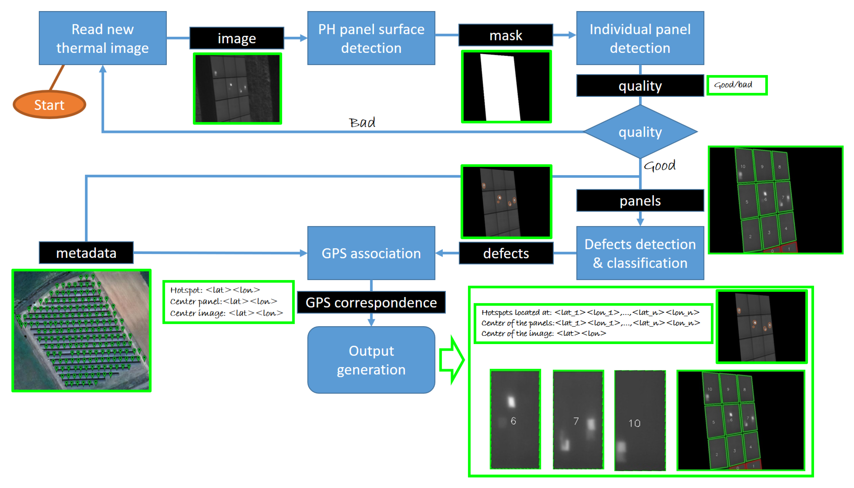
5. Automated Processing Procedure
The processing procedure can be seen in
Figure 9 and will be introduced as follows.
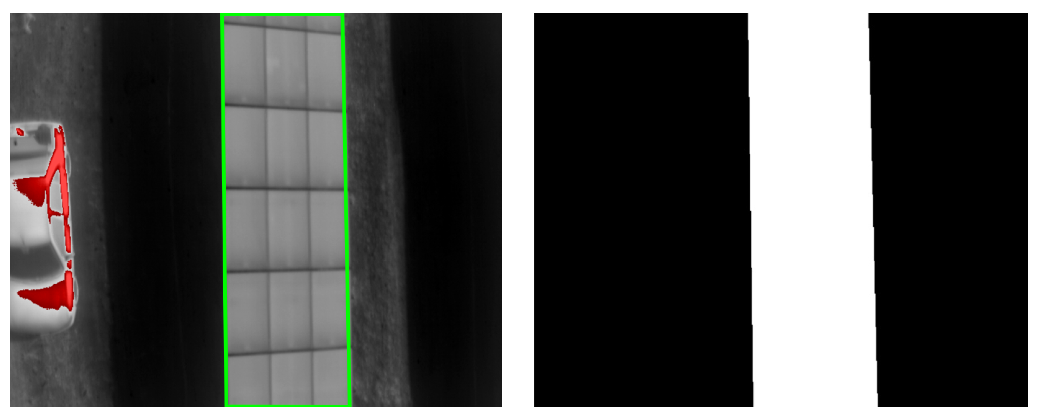
The system starts reading the thermal image of the camera, which is the input of the system. Once the image is read, the first step of the algorithm is to detect the surface of the panels. The purpose of this step is twofold. The first one is to make the algorithm more robust against abnormal elements or objects in the scene. The second one is to build a mask to be used in the next steps of the algorithm. An example that summarizes previous considerations can be seen in
Figure 10.
In
Figure 10 left, it can be seen that the hottest regions of the image are located over the car. However, if the panel surface is detected, these thermal abnormalities can be properly eliminated. The perimeter of the surface of the panels is highlighted (in green), and it can also be seen as an image mask in the right part of the Figure. For the detection of the panels surface, the K-means clustering algorithm [
26] is applied. More specifically, the thermal images are clustered into
k groups
according to the pixel intensities. Pixels that belong to a given cluster will be more similar in intensity than pixels that belong to a separate cluster. In this case, one cluster corresponds to the pixels of the background, the other cluster corresponds to the pixels of the panels shadows, and the last cluster of interest corresponds to the pixels on the surface of the panels. It should be noted that the pixels that belong to the panels surface is the cluster with the highest intensity. Therefore, it can be automatically identified.
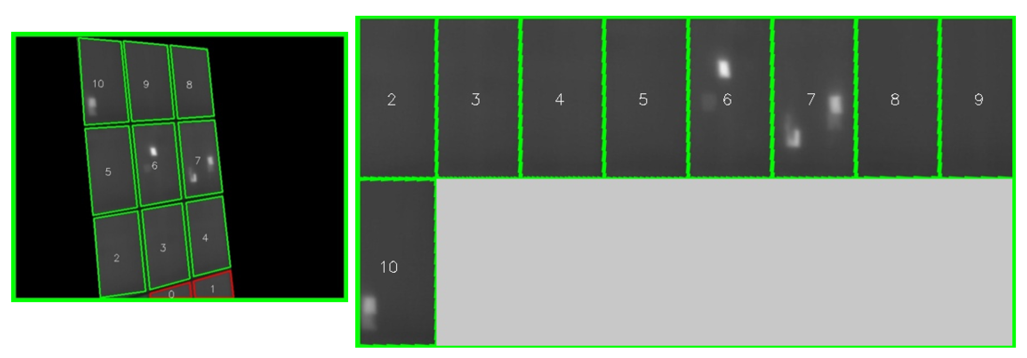
The second step of the algorithm is to perform the individual panel detection, which can be seen in
Figure 11. Given the original image (first image in
Figure 11), the algorithm tries to detect PV panels inside the mask (second image in
Figure 11). In order to do so, the first step is to detect the contours of the PV panels (third image in
Figure 11). The contours are obtained from the binary image after applying an adaptive thresholding technique [
27]. Once the contours are obtained, the next step is to correct the perspective distortion [
28] of all the detected contours. This procedure is done by calculating the best transformation matrix, which minimizes the error when correcting the perspective of all the contours in the image. The error is calculated taking into consideration the physical dimensions of a PV panel and calculating the difference (euclidean distance) between the four corners that define each contour and the four corners that define the PV panel. Therefore, this procedure is repeated as many times as the number of the detected contours in the thermal image. The transformation matrix with the lowest error is taken as the final transformation matrix and it is finally used to correct the perspective of all the contours (panels) in the image. It should the noted that, when the obtained error is too high, the image does not include panels. Therefore, this error can be used as a robust indicator to know whether the image contains PV panels or not. This step can be seen in
Figure 9 referred as ’quality’, and the result can be seen in the last image of
Figure 11, where the border of the image is green, which means that the error is low, indicating that this step of the algorithm detected panels inside the mask.
Additionally, it can be seen in
Figure 11 that the algorithm detects and identifies nine individual panels (marked in green) and also identifies two more panels (red) that are not completely seen in the image. The perspective corrected PV panels can be seen in
Figure 12. As commented before, this step is performed based on the real size of a PV panel. In this case, a PV panel has a size of 2 × 1 m.
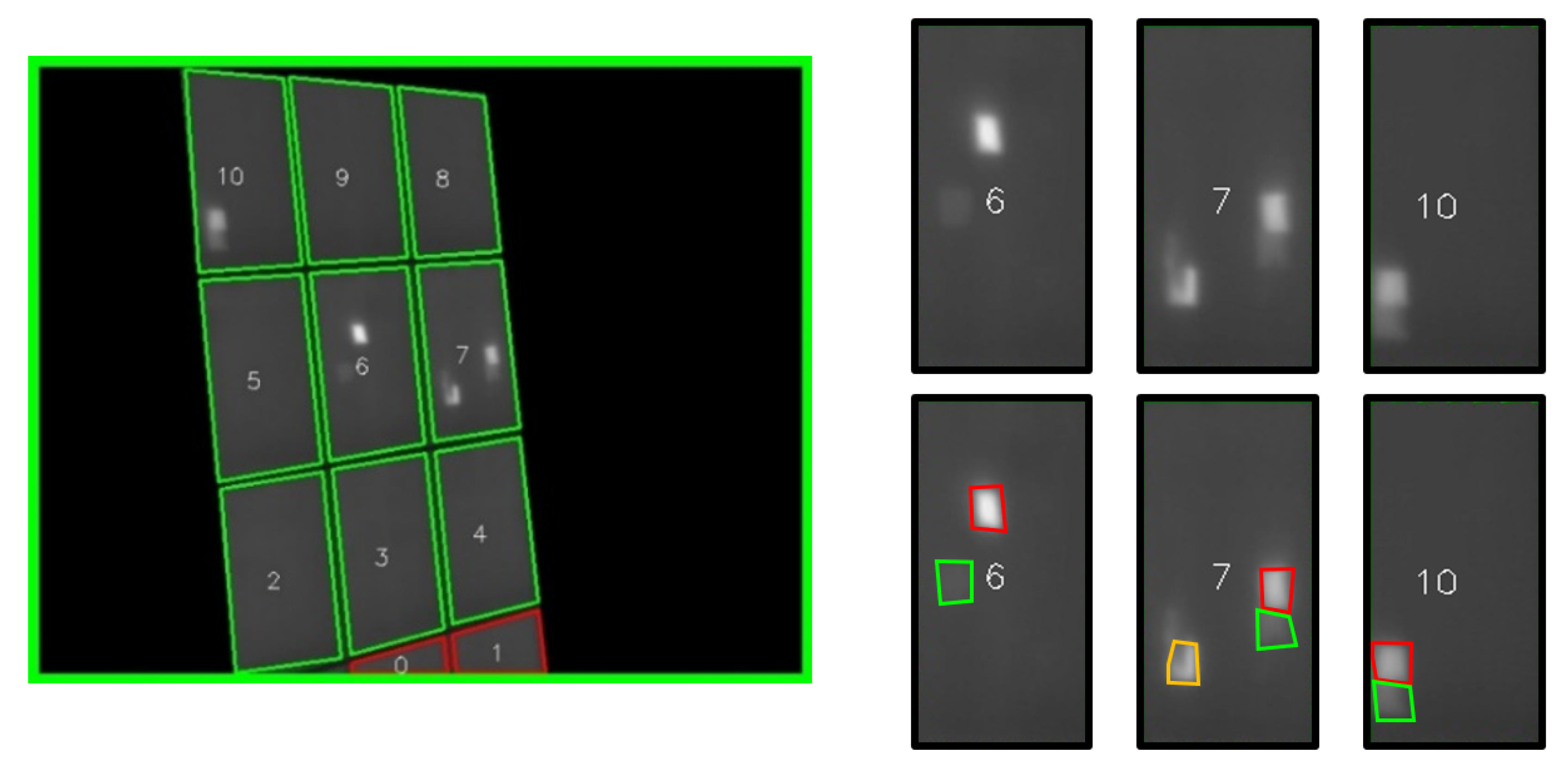
The correction of the perspective of the PV panels is a crucial step, because the correspondence between the pixels and the real positions inside the PV panel can be established. Once the panels are detected and the perspective is corrected, the next step is to independently detect the thermal defects in each panel. More specifically, each panel is treated as an independent image. In this publication, and according to the aforementioned considerations in the previous section, two different types of thermal anomalies are identified: (a) single-cell anomalies, and (b) module or row (sub-string) anomalies. Additionally, and according to the severity, the thermal defects are categorized into: (a) severe failures (differences higher than 30 °C), (b) medium severity failures (differences from 10 °C to 30 °C), and (c) minor failures (differences lower than 10 °C). This can be seen in the
Figure 13. Severe failures are shown in red, medium severity failures are shown in orange, and minor failures are shown in green.
The final step of the algorithm is to convert from pixel coordinates to GPS coordinates for every defect found in the image panels. A similar procedure than the algorithm proposed in [
29] is carried out. This way, a complete output is achieved containing both the GPS information of (1) every defect, (2) the center of each thermal panel, and (3) the center of the thermal image, and also all the generated images: (1) full thermal image and (2) the image of each thermal panel.
The images used for training and adjusting the parameters for the different steps of the algorithm were collected from previous UAV-based field inspections that were performed in two PV plants also owned by TSK. In these previous inspections, another camera was used, but the same GSD was achieved, decreasing the relative altitude of the UAV from the PV panels. More specifically, the FLIR VUE PRO camera was used. This camera is also based on an uncooled VOx Microbolometer providing a resolution of
pixels. This camera can be configured with three different lenses (9 mm, 13 mm, 19 mm). In these two inspections, the FLIR VUE PRO 13 mm was used, providing a FOV of
. The spectral band is also in the range of 7.5–13.5. In total, 500 images were collected with no overlap between them. In these images, a total of 63 hotspots and 15 bypass defects were manually identified. Finally, it should be commented that the acquisition of these images for training and adjusting the algorithms were necessary due to the lack of available public datasets, which is something that previous authors have also stated [
30].
6. Results and Discussion
The results are reported using standard metrics in a comprehensive way considering a total of 321 thermal images.
The number of defects found in this PV plant is way larger than the average number of defects found in other PV plants that were owned by the company. The reason for using this PV plant as a dataset is to have enough defects to evaluate the developed algorithms.
6.1. Results in the Segmentation of the Panels Surface
A robust segmentation algorithm of the surface of the panels is crucial. This way, all of the thermal defects found in the images are located inside the surface of the panels. Segmentation performance is commonly evaluated with respect to Gold Standard (GS) manual segmentation performed by a human expert. Furthermore, a combination of segmentations by multiple
experts is usually employed to attenuate intra-subject variability when performing the manual segmentation of
images and obtain a truthful GS. In this sense, different strategies have been proposed to combine the segmentations. In this case, the Simultaneous Truth and Performance Level Estimation (STAPLE) approach is used [
31]. When evaluating the performance of segmentation algorithms with respect to GS, a contingency table considering True Positive
, True Negative
, False Negative
, and False Positive
is commonly used, where positive and negative refer to pixels belonging to panels and background, as in accord with the GS segmentation, respectively. Based on this table, Accuracy
, Sensitivity
, and Specificity
are the most frequently adopted measures, where
is the proportion of true results, both
and
, among the total number of examined cases
.
, also referred as
rate, measures the proportion of positives, both
and
, which are correctly identified.
measures the proportion of negatives, both
and
, which are correctly identified. A formal definition of the aforementioned measures used for evaluating the results in the segmentation of the surface of the panels can be seen in (
7). For the evaluation of the segmentation algorithm of the panels surface,
,
.
Based on the values included in
Table 2, the obtained results are:
,
, and
, showing that the proposed algorithm for the PV panels surface detection is adequate for filtering the thermal defects inside the PV panels.
6.2. Results in the Binary Classification of the Images (Images with/without Defects)
The idea behind this classification is that the operators will only review images that have triggered one or more thermal defects by the algorithm. This is because, by average, there are many more images without defects than images containing defects, and the fact that the operator will review the images only containing defects is faster than reviewing both the negative images (images without defects) or even all of the images. Therefore, this can be seen as a two-class classification problem. In this case, positive refers to a thermal image with one or more defects, while negative refers to a thermal image with no thermal defects. In a similar fashion as in the previous sub-section, Accuracy , Sensitivity , and Specificity can be calculated. In this case, all of the thermal images (321) are considered for the evaluation of this binary classification.
Based on the values that were included in
Table 3, the obtained results are:
,
, and
. These results show that the binary classification of the images can be an efficient way of automatically filtering all of the images allowing the operator to only review the positive images due to the high specificity of the proposed processing procedure.
6.3. Results Detecting the Thermal Defects of the Images
When evaluating an algorithm in the context of object detection, some concepts and metrics should be properly defined forehand. Intersection Over Union
is measured based on Jaccard Index that evaluates the overlap between two bounding boxes. It requires a ground truth bounding box and a predicted bounding box.
is calculated as the area of the overlap divided by the area of the union. By comparing the
with a given threshold
t, a detection can be classified as being correct or incorrect. In this context, a
is considered as a correct detection of a ground-truth bounding box (detection with
), a
is considered as an incorrect detection of a nonexistent object or a misplaced detection of an existing object (detection with
), and
is considered as an undetected ground-truth bounding box. It is important to note that, in the object detection context, a
result does not apply, as there is an infinite number of bounding boxes that should not be detected within any given image. For evaluating the algorithm, the threshold
t was set to
. The standard metrics are precision and recall in order to evaluate an object detection algorithm [
32].
Precision is the ability of a model to only identify the relevant objects. It is the percentage of correct positive predictions. Recall is the ability of a model to find all of the relevant cases (all ground truth bounding boxes). It is the percentage of true positive detected among all relevant ground truths. A Precision of 0.976 and a Recall of 0.923 are achieved detecting the thermal defects of the images.
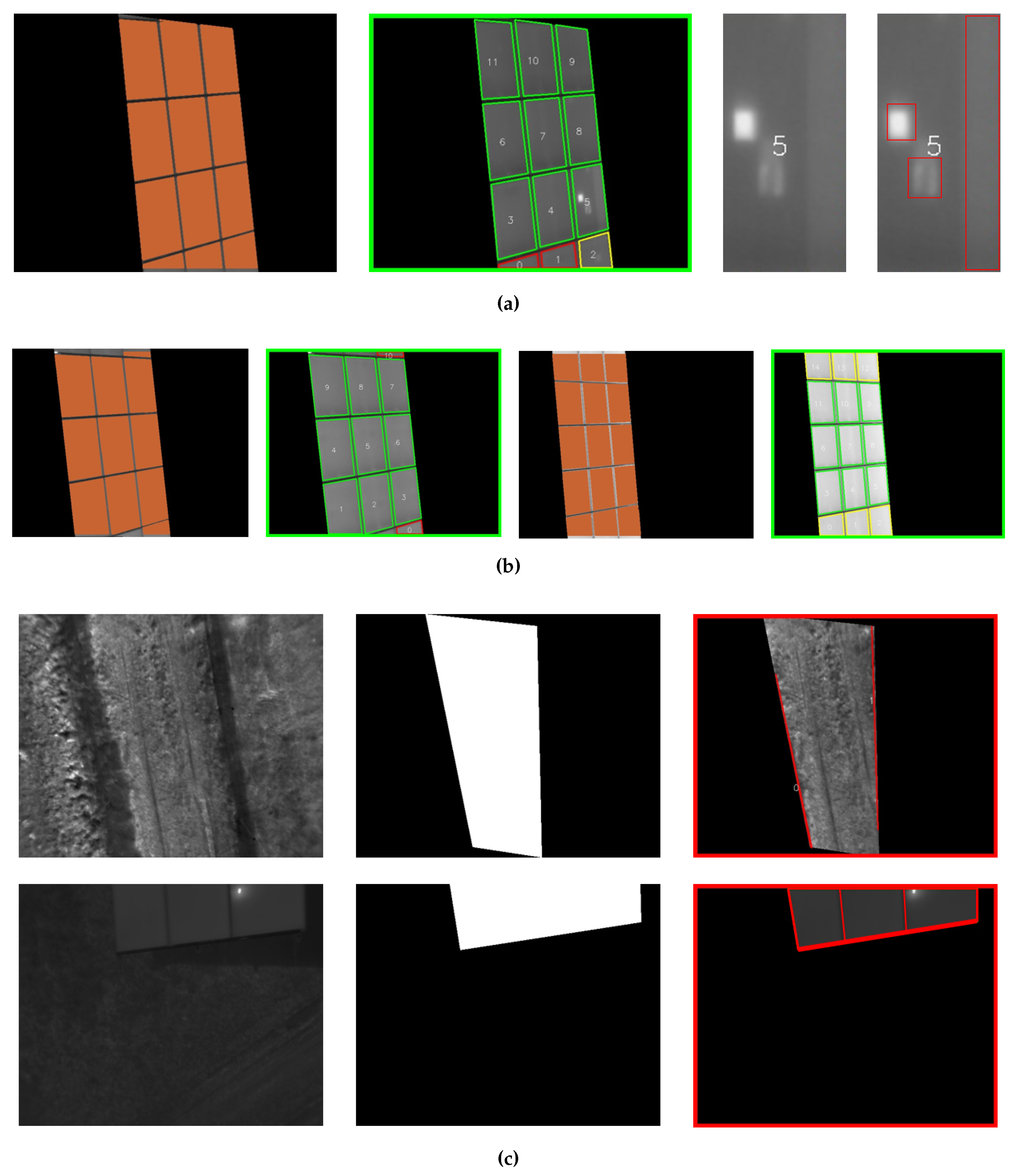
Figure 14 provide a qualitative perspective of the results included in these previous subsections.
More specifically, in
Figure 14a, the results detecting the thermal defects are shown. In can be seen that all of the thermal defects are identified. Additionally, the image has also been classified as correct, because the calculated error after correcting the perspective of all the identified PV panels is low.
Figure 14b shows two images without thermal defects, reflecting that the operator will only review positive images (containing defects) and, hence, will not review negative images.
Figure 14c shows two images where the processing procedure calculated a high error when correcting the perspective of the detected PV panels. In both cases, the images do not contain full PV panels. In
Figure 14c, the first image corresponds to the background. Many images captured by the UAV only contains background. Additionally,
Figure 14c shows a second image where not the PV panels are fully registered. In both cases, the processing procedure does not continue processing the images.
The proposed algorithm can provide state-of-the-art results in the context of detecting, classifying and geopositioning thermal defects. Based on the review of the literature, and as far as the authors know, this is the first time that the surface of the panels is detected. This way, all of the thermal defects that can be potentially detected by the next steps of the proposed system are located inside the panels. Hence, many false-positive thermal anomalies can be efficiently eliminated. Moreover, this is also the first time that the panels are perspective corrected. Applying perspective correction, the geometry of the thermal defect can be properly obtained. Furthermore, this is also the first time the thermal defects are automatically geopositioned. This way the latitude and longitude of every defect can be automatically obtained. In a previous work ([
10]) the defects are manually located. Therefore, the operator needs to manually assign the exact location of each fault to the individual PV module.
Finally, and for the sake of completeness, some images that were not correctly processed by the system are included. More specifically, both
Figure 15 and
Figure 16 have been included. In
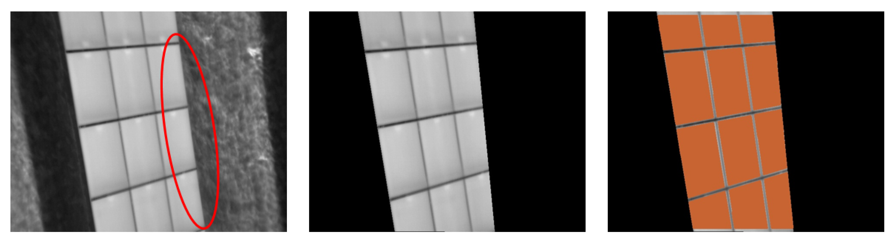
Figure 15, it can be seen that the segmentation of the panels was not correctly performed. In this sense, this initial segmentation of the panels surface affects the detection of three individual panels.
In
Figure 16, it can be seen that, despite the fact that the system performs an accurate segmentation of the panels and also a good identification of the individual panels, one cell that is warmer than the others (in panel 5) is not detected. Additionally, the system only detects a single cell instead of a one row that is warmer than the other rows in the module (in panel 9).
7. Conclusions
It is essential to monitor the health status of the PV system in order to identify and locate premature faults that could severely affect the output power generation. IRT imaging is the gold standard to identify, classify and locate defect(s) or defective PV module(s). However, ground-based IRT imaging analysis performed by qualified operators is a time-intensive complex inspection process that increases the operation costs. Moreover, it is impractical for the inspection of large-scale PV systems.
Therefore, the adoption of UAV-based approaches is justified. However, the implementation of a cost-effective method to scan and check huge PV plants represents major challenges, such as the cost and time of detecting PV module defects with their classification and exact localization within the solar plant. Moreover, many technological considerations should be taken into account for a proper inspection of photovoltaic plants. In this work, a fully automated approach for the detection, classification, and location of the thermal defects in the PV modules is carried out. In this work, a robust and comprehensive procedure is proposed, providing innovative characteristics not addressed before in the literature. The system has been tested in a real large PV plant owned by TSK company, showing that the proposed system can be used for a proper automated thermal inspection of PV plants.


 ,
, 


