Fast and Improved Real-Time Vehicle Anti-Tracking System

Abstract

Safety on roads and the prevention of accidents have become major problems in the world. Intelligent cars are now a standard in the future of transportation. Drivers will benefit from the increased support for driving assistance. This means relying on the development of integrated systems that can provide real-time information to help drivers make decisions. Therefore, computer vision systems and algorithms are needed to detect and track vehicles. This helps traffic management and driving assistance. This paper focuses on developing a reliable vehicle tracking system to detect the vehicle that is following the host vehicle. The proposed system uses a unique approach consisting of a mixture of background removal techniques, Haar features in a modified Adaboost algorithm in a cascade configuration, and SURF descriptors for tracking. From the camera mounted at the rear of the host vehicle, videos are captured. The results presented in this paper demonstrate the potential and efficiency of the system.

1. Introduction

As the number of vehicles increases, the demand for driver assistance systems also increases, ensuring safe and comfortable driving. Over the last decades, many criminals have been resorting to the method of stealing cars commonly referred to as carjacking. This most frequently happens while the owner is driving the vehicle and is temporarily stopped, e.g., at a traffic light, gas station, convenience store, ATM, hotel, etc. Carjacking can be prevented by equipping a vehicle with an anti-tracking system which alerts the victim vehicle to being tracked by suspicious criminals.

From this perspective, the intelligent transportation industry has conducted various studies. This is achieved by installing high-tech equipment and other control systems on the vehicle rather than on the road. In this case, many visual sensors are used [1]. The vision system installed in the transport vehicle can provide the location and size of other vehicles in the traffic environment, as well as provide information from roads, traffic lights, and other road users. All this information captured by the vision system is very useful in the event of traffic incidents (such as an accident or carjacking) [2].

The proposed system uses information from the visual system represented by one camera. This provides a picture and video of the scene behind the car. The purpose of the system is to identify vehicles located in this space and following the host vehicle. However, some factors are obstacles to the reliability and robustness of the tracking system, such as:

(1)

Occlusion. Some parts of the vehicle of interest may be blocked by objects or other vehicles [3]. In our application, placing the camera behind the car will create many occultations between the vehicles.

(2)

External conditions. Color, intensity, texture, and lighting vary from image to image. The following vehicle is subject to many variations; not only the extrinsic changes produced by the visual system (lighting conditions, location of the camera), but also the intrinsic differences in the vehicle type (color, height, etc.) must be taken into account [4].

(3)

Position of the object of interest. In an image, a vehicle can be seen from the front, in profile, or from any angle. The system must also be able to deal with low-resolution images, which usually make it difficult to detect and recognize an object accurately [5].

(4)

Computation load. The exhaustive search of potential positions of vehicles in the full picture is prohibitive for real-time applications. The response speed is measured, in fact, for the entire system: most of the execution of all processes is done in “real-time”. Here, the term implies that the system is capable to detect and recognize a following vehicle present in the vehicle environment before it reaches it, so the driver is warned of a dangerous situation.

Many researchers have tackled these issues in their work to get better results. Keyu et al. proposed a method based on there being motion in an image [6]. In such a case, the intensity value of a pixel will be different from the corresponding pixel in the next frame or the reference frame. Generally, the subtraction of the background is achieved as follows: An initial model is created to model the background image. The difference between the current image and the background model is estimated to spot moving objects; and finally, the background template is updated. The regions thus detected form probable objects of interest. Ekta Saxena et al. proposed an object tracking algorithm that takes an image from a camera and converts it to a pre-processed image in grayscale [7]. Then the image goes through the process of canny-edge detection. If the number of vehicles is large enough after filtration and expansion, that area is selected and vehicles are detected on the image in the form of a bounding box. Finally, the algorithm uses a blob analysis for the detection of a separate number of vehicles. Yingfeng et al., to update the background model, based their approach on the texture of the image, using processing such as the texture-based moving object detection method (TBMOD), in which each distribution is adjusted by weight [8]. The TBMOD models each pixel by a binary pattern calculated by a comparison between a pixel and its neighborhood. More specifically, a histogram is associated with local patterns in a circular region. Then the decision is determined by comparing the various histograms. Mahabir et al. have developed a technique to detect and recognize vehicles from RGB images using image morphology and target spectra [9]. The quality result of the detection process is 65% higher and false detection occurs when using a car with sunlight and spectral values. Engel and his team proposed a multi-object tracking approach which is based on a cascade filter of detector objects [10]. This filter is made up of the following constraints: the size of the objects, the weighting of the background, and the smoothness of the trajectories of the target objects.

The performance of the whole of the developed systems depends on the results provided in the output of the processing chain. This corresponds to the results of good recognition of vehicle shapes. The goal of the method proposed in this paper is to first develop an anti-tracking system, which is a combination of detection and recognition of following vehicles, capable of detecting a following vehicle at any time. The second goal is to improve the speed and accuracy of such a vehicle tracking system. Achieving this second goal involves making choices of methods in terms of execution time; a method is required that is capable of detecting and recognizing multiple vehicles without error, and in real-time speed. The system will then be evaluated through standard performance measures, comparison with other similar systems, its effectivness against occlusion, and its effectiveness when presented with different vehicle shapes as well as varying external conditions.

2. Proposed Model

As shown in Figure 1, the main steps of the system are as follows.

2.1. Data Preprocessing

As mentioned before, different algorithms and methods used or made will have to be inexpensive in computing time at runtime. Digital images, as they are acquired from the camera, are very often unusable for image processing—they include noisy signals. To remedy this, as shown in Figure 2, we use the following pretreatments:

• Resizing: Due to the large number of digital cameras sold, the development of sensor technology has led to the emergence of many new products, including those with an increase in the number of sensor pixels. Having a high-quality camera is good for the eyes, but image processing does not always benefit from larger image sizes. A large number of pixels will quickly cause a large number of mathematical operations, resulting in a large number of calculations on the computer. Resizing the image is desired to improve computation. Figure 3 shows an example of adjusting the image from 240 × 360 to 190 × 290. The subject in question is still clearly visible. This is because each pixel must be processed when starting to process the image.
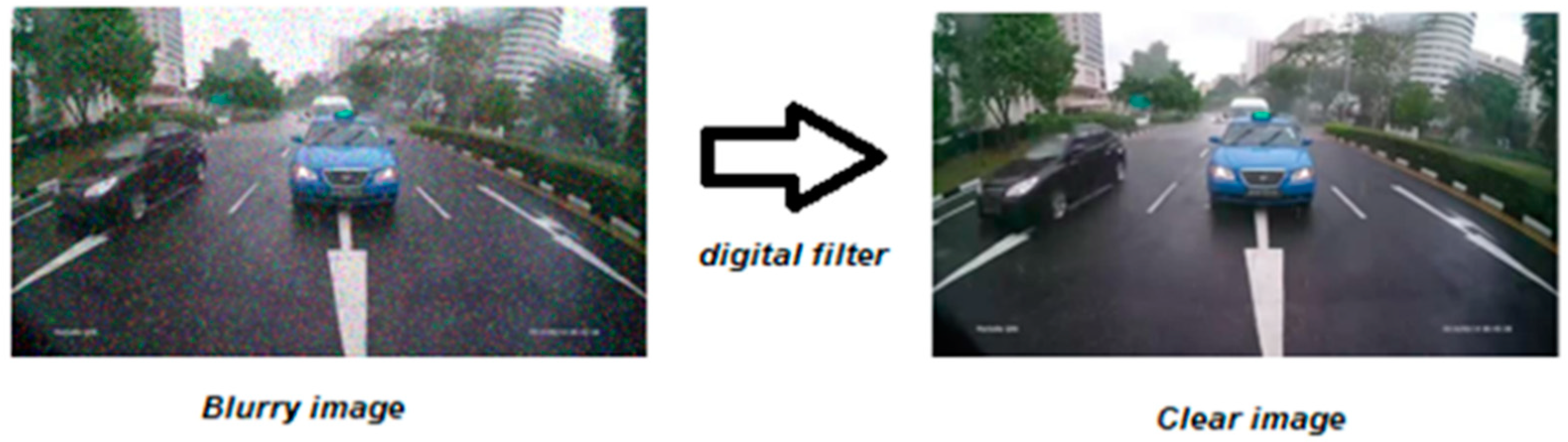
• Noise removal: To manipulate an image, we work on an array of integers that contains the components of each pixel. The treatments always apply to grey-level images, and sometimes also to color images. To improve the visual quality of the image, we must eliminate the effects of noise (parasites) by making it undergo a treatment called filtering (Figure 4). The filtering consists of modifying the frequency distribution of the components of a signal according to given specifications. The linear system used is called a digital filter.

2.2. Vehicle Detection

2.2.1. Adaboost Cascade Classifier with Haar Features

The initial detection system uses the Adaboost cascade classifier with Haar features. To do so, a sample of an image is used to extract those features (Figure 5). This process considers the adjacent rectangular areas at a specific position in the detection window, then adds the intensity of the pixels in each area and calculates the difference in size.

The use of integrated AdaBoost is a form of “general learning” that uses multiple learners to create more powerful learning algorithms. AdaBoost works by selecting a basic algorithm and optimizing it by reporting examples of wrong classifications in the training set [11]. The entire training model is given the same initial weight, and the basic algorithm is selected to train the weak learners. As a result, the weight of the incorrect samples increases. Each time, the primary learner uses the updated weight on the training set, and the training is repeated n times. The final decision is to determine the total weight of n learners.

The Adaboost steps [12] can be summarized as follows:

• Given example images $(x_1, y_1)\dots .(x_n, y_n$) where $y_i$ = 0, 1 for negative and positive examples respectively.
• Initialize weights $w_{1,i}$ =$\frac{1}{2m}$ or $\frac{1}{2l}$ for $y_i$ = 0 or 1, respectively. The variables $m$ and $l$ are the numbers of negatives and positive, respectively.
• For $t=1,\dots ,T:$
  • Normalize the weights,

    $$w_{t,i}\leftarrow \frac{w_{t,i}}{{{\displaystyle \sum }}_{j=1}^n{w}_{t,j}}.$$

    (1)
  • Select the best weak classifier for the weighted error:

    $${ϵ}_t=mi{n}_{f,p,\theta }{{\displaystyle \sum }}_i{w}_i\left|h\left(x_i,f,p,\theta \right)-y_i\right|.$$

    (2)
  • Define $h_t\left(x\right)$ = $h\left(x,f_t,p_t,{\theta }_t\right),$ where $f_t,p_t$ and ${\theta }_t$ are the minimizers of ${ϵ}_t$.
  • Update the weights,

    $$w_{t+1.i}= w_{t,i}{\beta }_t^{1-e_i},$$

    (3)

    where $e_i=0$ if example $x_i$ is classified correctly, $e_i=1$ otherwise, and ${\beta }_t=\frac{{ϵ}_t}{1-{ϵ}_t}$.
• The final strong classifier is

  $$C\left(x\right)=\{\begin{array}{c}1, if {\displaystyle \sum }_{t=1}^T{\alpha }_t{h}_t\left(x\right)\ge \frac{1}{2}{\displaystyle \sum }_{t=1}^T{\alpha }_t\hfill \\ 0, otherwise\hfill \end{array},$$

  (4)

  where ${\alpha }_t= log\frac{1}{{\beta }_t}$.

To achieve this overall learning strategy, many classifiers are combined, and each classifier is based on the results of one or more Haar features. The cascade classification includes a list of steps, and each step includes a list of weak learners. The algorithm detects cars by placing and moving sliding windows on the image. Each stage of the classification denotes the specific area defined by the current sliding window position as positive (vehicle detected) or negative (vehicle not detected) (Figure 6). If the marking result is negative, the classification of this specific region is now complete and the sliding window position moves to the next position. If the mark gives good results, the area (32 × 32 numbers) will move to the next classification step. Objects are identified as they go through all stages of classification. This document focuses on three steps.

Further modifications were done to improve the speed and accuracy of the system.

2.2.2. Background Removal

Segmentation is one of the critical steps in image analysis that determines the quality of subsequent measurements. Segmentation makes it possible to isolate in the image the objects on which the analysis must be made, thus separating the regions of interest from the background. Traditional background removal techniques have been developed based on the simple static background method [13]. This is because if the images have the same static background (such as a video taken from a CCTV camera on the road or a fixed room), the foreground and background can be separated. However, in our case, the background is constantly changing. So we have our unique approach to detect the region of interest.

The area of search on the image is limited by the use of the general knowledge of a street perspective. Vehicles cannot be found in the sky or a building—they are always on the street. Then, the image is analyzed through a moving window and is assessed by a detector of a different resolution, a multiple of 32 × 32. This is the smallest resolution allowed for a recognizable car. Vehicles are only detected and tracked as they enter a region of interest (ROI); when vehicles leave the ROI line, tracking stops. To track the region of interest, boundaries around vehicles are created, and the process continuing.

To determine the exact location of the region of interest, we run the dummy vehicle detection software on the system while on the road. We detect vehicles and we notice that all the vehicles are located in a certain region. The heat map result shows that for an image of 620 × 340 pixels, the vehicles are located in the region of interest, as shown in Figure 7, inside the yellow rectangle, between y1 = 100 and y2 = 300. If this area of the frame is the only field of view, we will obtain the best output. Of course, this depends on the placement of the camera and the angle of view, which cannot be changed.

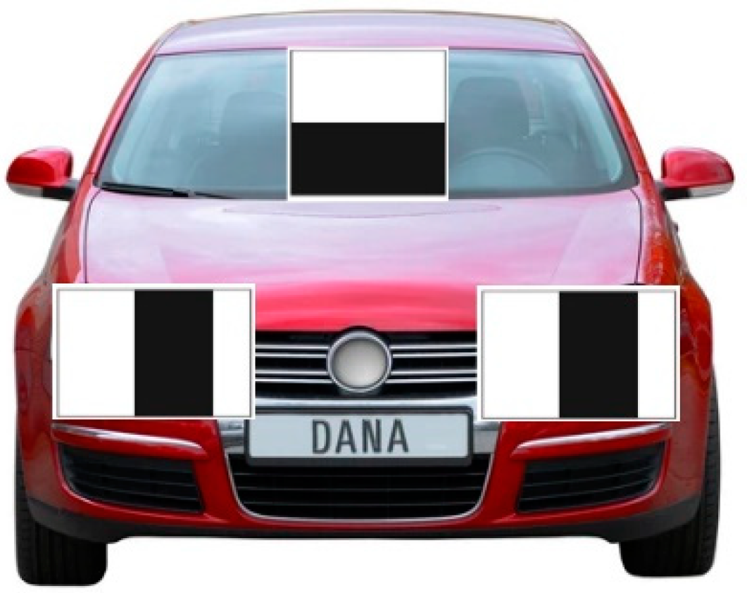
2.2.3. Front View of the Vehicle

The goal of the system is to track vehicles that might be following us. We should not be paying attention to vehicles that are still or are going in the opposite direction. To achieve that we feed more front-views of vehicles into the positive samples database and, together with the narrowed region of interest, we increase the robustness of detecting the following vehicle as the overall computation time of the algorithm is reduced and accuracy of the overall system is increased. Figure 8 shows examples of images of the front-views of vehicles added in the positive samples database and needed to improve the accuracy and robustness of the system.

2.2.4. Feedback System

We insert a road test shot set into the AdaBoost classifier. The AdaBoost classifier generates refined search results with both positive and negative images. We use these results as reference input. As shown in Figure 9, the positive database has been reconstructed with positive results from the previous steps. However, the negative database has been reconstructed as a negative result of the previous step. Negative results were street signs, such as railings and traffic signs. Rare image patches on common roads such as signs, buildings, and skies are excluded. We used the output from the previous step to re-learn the classifier, creating the correct classifier. The performance of the categorizer has been improved over previous steps whenever the database has been rebuilt.

Additionally, in the online mode, we run the software with actual footage we recorded with our camera, bearing in mind that people usually use the same roads in their daily activities. We, therefore, run our algorithm on the video recorded going to all those places, and save all negative samples in the “experimental negative sample”. These samples are fed back to the original cascade. In so doing, we again increase the accuracy of the detection.

2.3. Vehicle Recognition

Tracking is the process of recognizing a previously detected vehicle at any following frame. Template-based object matching is the method mostly used when you have two objects of the same nature, but we need a fast scale-invariant method. Therefore, we use the speeded-up robust features (SURF) algorithm for the template matching. The SURF algorithm is faster and more accurate than template-based methods and proves to be more robust as regards certain transformations. This method includes three steps: extraction of points of interest, calculation of descriptors, and matching of points of interest (Figure 10).

The SURF method uses the fast-Hessian algorithm for the detection of points of interest and an approximation of the Haar features to calculate the descriptors (Figure 11) [14]. They make it possible to estimate the local orientation of the gradient and therefore to provide the invariance concerning the rotation. The responses of the Haar features are calculated in x and y in a circular window whose radius depends on the scale factor of the point of interest detected. These specific responses contribute to the formation of the characteristic vector corresponding to the key point. Regarding the matching of descriptors (Figure 12), i.e., the search for the best similarity between the descriptors of two images, the criterion used is the same as that used in most algorithms, the Euclidean distance.

We have applied the algorithm to a video sequence containing vehicle images. The training database consisted of previously detected vehicles and the test image is the newly detected vehicle. In our detected vehicle database, we already have a template of the vehicle. Therefore, there is no need to crop the vehicle image or subtract the background. We need to minimize the computational time, as the detected vehicle database will increase with time. This causes the recognition system to become slower and slower over time, because of the number of detected vehicles stored in the database.

Therefore, our system will complete the recognition process after 30 s minimum, as there is generally not much change in the camera view for vehicles going in the same direction. We will maintain the assumption that all vehicles will follow our host for a minimum of 30 s to be considered as a potential follower. Also, we have decided to separate the recognition system from the detection system. In doing this, we are able to recognize all previous detected vehicles without interfering with the tracking process. Figure 13 shows the combination of the detection and recognition phases, without them interfering with one another.

2.4. Vehicle Anti-Tracking

The goal of the research was to study the possibility of developing an anti-tracking system for vehicles on the road. This means detecting and tracking pursuing vehicles, and recognizing them if they have been following the host for a long time. We use output data from the combination of the detection and recognition systems to inform the host that it might be followed by another vehicle. After detected, all vehicles are placed in the detection database, and each newly detected vehicle is compared to the ones in the detection database; those that match are placed in the recognition database.

When the same vehicle has been recognized for over two minutes, it is labeled as a potential suspicious follower and the host vehicle driver can be alerted to pay attention to that vehicle via a simple alarm system connected to our system. Data on the following vehicle can be used in case of any criminal activity occurrence. Figure 14 shows the example of the yellow vehicle being detected at frame t, and the same vehicle is detected again and recognized by the system every 30 s for a total of two minutes and is labeled as a potential pursuer.

3. Implementation and Results

For our study, the acquisition of video sequences is realized through the vehicle’s rear-mounted camera. This allows us to quickly obtain a significant amount of data, thus being able to track signals. The video feeds are captured at various locations at different times of the day. The height of the mounted camera is unknown. Initial testing of our algorithms and methods described in this paper was conducted using a dataset found on the internet. We also used video footage of traffic recorded from the rear of vehicles to perform the preliminary tests. These footages were found on YouTube. For a practical experiment, 5 videos were recorded on the streets of Pretoria, South Africa. Approximately 1560 frames of the traffic environment are used as positive images, and 2000 are used as negative samples. Some negative samples came directly from our experiment. All identified vehicles are labeled “cars” and are enclosed in rectangles (Figure 15); a vehicle being tracked is enclosed in a red rectangle (Figure 16). Using axial symmetry, the positive sample array is multiplied by the mirror image composition. Of the 31,200 images, two-thirds are used for the positive training set, and the rest are used for the positive verification set. The latter is used to set the classification threshold based on the correct detection rate and the false-positive rate.

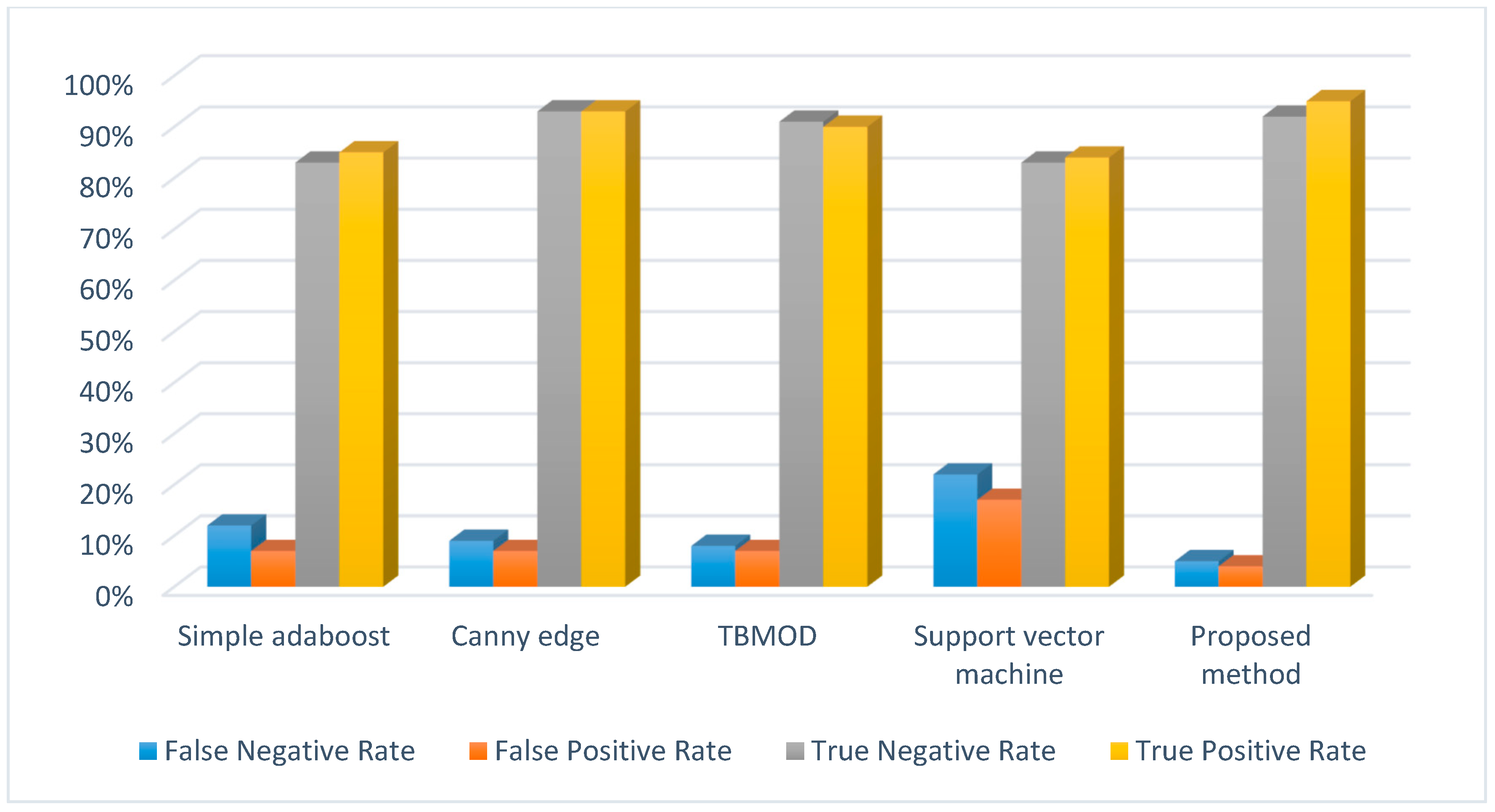
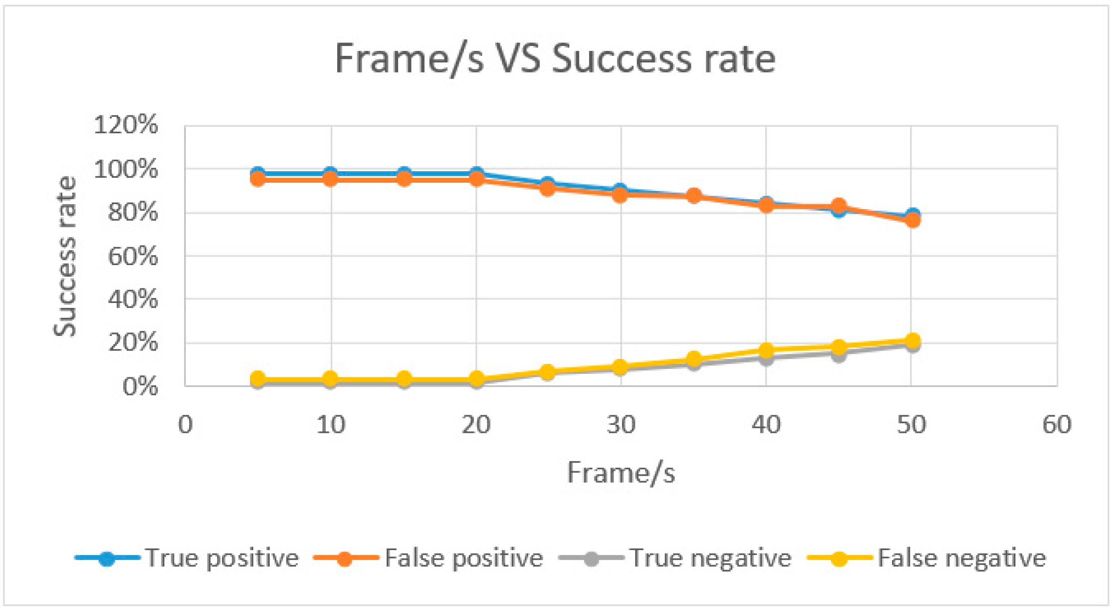
3.1. Detection System

Figure 17 shows the rate of false negatives (FN), false positives (FP), true negatives (TN), and true positives (TP) in the system’s vehicle detection success rate. The proposed method has a high success rate in both positive and negative results, which means high reliability. The success rate is calculated by the following formulas:

True-Positive Rate = TP/TP + FN
False-Positive Rate = FP/FP + TN
True-Negative Rate = TN/TN + FP
False-Negative Rate = FN/FN + TP

For good classifiers, TPR and TNR both should be near to 100%. On the contrary, FPR and FNR both should be as close to 0% as possible.

The proposed system is also compared to other methods that give the best results. We applied their concepts and algorithms to our system under the same circumstances and compared the overall results. The total system computation time of the proposed multi-vehicle detection system is up to 51 ms, and it is possible to operate perfectly at a frame rate of up to 30 frames per second.

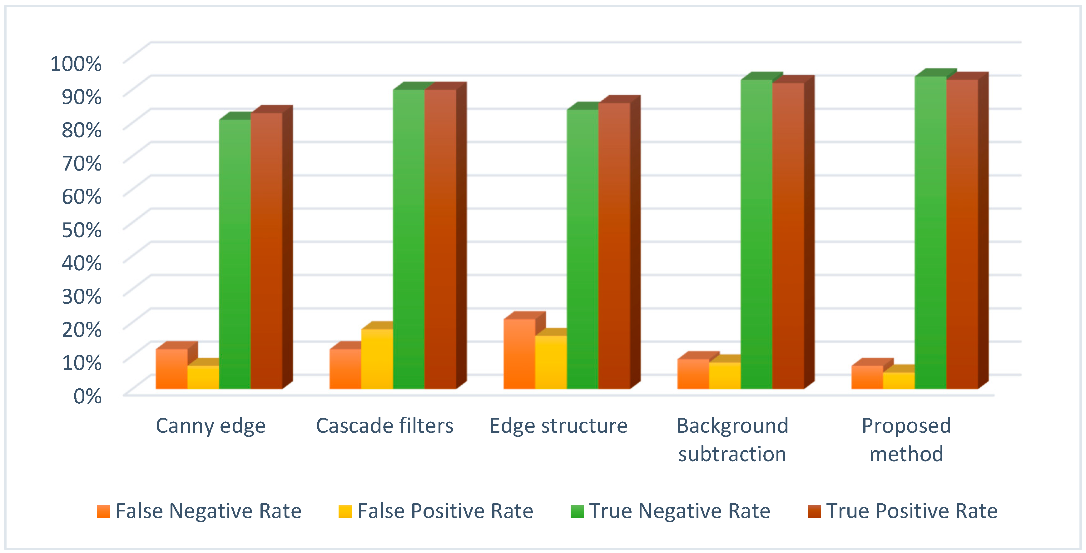
3.2. Recognition System

The tracking results are also very accurate (Figure 18). As stated, in the tracking phase we used the SURF method on our detected vehicles database to recognize a newly detected vehicle. What sets our approach apart from other techniques, is that the detected database is made up completely of already cropped vehicle images. There is no need to remove any other unwanted object in the picture. This leads to less time in computation, and less error in the recognition accuracy.

3.3. Overall System Performance

● Occlusion

For the relevant representation of the signature of a vehicle in the recognition phase, the SURF descriptor, which allows extracting characteristics invariant to scale and object rotation, is applied to detect points of interest of vehicles and to extract characteristics around these points. The SURF algorithm was used, but gave even better results because the training–image database only had vehicles stored in it. There was no background removal technique needed, nor cropping methods. This saves a great deal of time on the overall duration of the algorithm, which is what we wanted. The recognition system was very effective against the presence of occlusions and different viewing angles in the images; it was able to find a match with a very high threshold.

● External Conditions

Each video is recorded in different places and in different scenarios. Part of the scenario suffers from a lack of accuracy. In the rainy scene (Video 5) various lights shine on the vehicle, and rain falls on the camera accidentally; due to unstable shots, owing to camera shake, the success rate decreased to 90%, which is still good. The resolution of this video sample is set to 320 × 240, and the duration is set to 180 s. Sample results for all of the subsystems are presented below (

Table 1. Overall system performance.

Video	Frame Rate (fps)	Total Vehicle	Detction Success Rate (%)	Tracking Success Rate (%)
Video 1 (Sunny)	25	37	100	100
Video 2 (Sunny)	25	18	100	100
Video 3 (Sunset)	30	52	97	95
Video 4 (Foggy)	30	45	97	92
Video 5 (Rainy)	35	22	94	90

).

● The Shape of the Object

Figure 19 shows that the system is effective for various categories of vehicles. We then examine the vehicle types’ detection success rate. It is important to highlight that we did not work on vehicle classification. This is merely to see how effective our algorithm is when it needs to detect a car, truck, or bus. The results obtained are more or less what was expected. Normal-sized vehicles have a higher chance of being detected than the remaining types, because of their small size. For the training database, we used a large number of normal-sized vehicles (70%) compared with truck images (13%) and bus images (17%). Balancing the database will certainly increase the success rate of both trucks and buses; however, the results obtained are already more than satisfactory.

Recognition results are a little less impressive compared with the detection because of the color dilemma. In one video, we had two identical vehicles with the same color and it was difficult to identify which vehicle was detected previously. The result gave a high threshold value for both, and of course one will be considered a false positive and the other a true positive, thus impacting the statistics.

● Real-Time Performance

One of the most important aspects of our research has been the real-time element and the overall computation time of our system. Our system started showing some performance issues when we increased the frame rate of the videos. However, with a frame rate under 30 fps, the system gives excellent results, as shown in Figure 20.

4. Conclusions

The experimental results obtained show that our system of tracking presents the best results by using the Adaboost algorithm and SURF algorithm to detect a possible following vehicle. The proposed anti-tracking system has three mains parts: preprocessing, detection, and recognition. In the detection work, the proposed method was based on the AdaBoost algorithm with three cascades of classifiers (front view, left profile, and right profile) to detect vehicles in the video sequences. This algorithm, combined with good input image processing, is fast and robust in its ability to detect vehicles of different shapes and different brightnesses. The combination of three cascades allows us to obtain a higher rate of good detections. The SURF algorithm was used to detect previously detected vehicles in a new frame. An improvement can be made by enriching the base of images of different positions and rotations to cause several cascades of different poses—but that was not enough. We needed to find a system robust and accurate enough for our objective, so we improved the algorithm with a precise positive dataset, a feedback system, and a new segmentation method that gave us excellent results. Finally, the anti-tracking system determines which vehicle is a possible follower by running the recognition system every 30 results. The vehicle that is repeatedly recognized by the system is labeled as a potential pursuer. Further improvement to this project to get even more impressive results would be to associate a license plate recognition system to our tracking system to remove the vehicle color complexity.

References

1. Guvenc, I.; Koohifar, F.; Singh, S.; Sichitiu, M.L.; Matolak, D. Detection, tracking, and interdiction for amateur drones. IEEE Commun. Mag. 2018, 56, 75–81. [Google Scholar] [CrossRef]
2. Yang, L.; Luo, P.; Loy, C.C.; Tang, X. A large-scale car dataset for fine-grained categorization and verification. In Proceedings of the 28th IEEE Conference on Computer Vision and Pattern Recognition (CVPR), Boston, MA, USA, 7–12 June 2015; pp. 3973–3981. [Google Scholar]
3. Milan, A.; Leal-Taixe, L.; REID, I.; Roth, S.; Schindler, K. MOT16: A benchmark for multi-object tracking. CoRR 2016. [Google Scholar]
4. Ofor, E. Machine Learning Techniques for Immunotherapy Dataset Classification. Master’s Thesis, Near East. University, Nicosia, Cyprus, 2018. [Google Scholar]
5. Yildrim, M.E.; Ince, I.F.; Salman, Y.B.; Song, J.K.; Park, J.S.; Yoon, B.W. Direction-based modified particle filter for vehicle tracking. ETRI J. 2016, 38, 356–365. [Google Scholar] [CrossRef]
6. Lu, K.; Li, J.; Zhou, L.; Hu, X.; An, X.; He, H. Generalized haar filter-based object detection for car sharing services. IEEE Trans. Autom. Sci. Eng. 2018, 15, 1448–1458. [Google Scholar] [CrossRef]
7. Saxena, E.; Goswami, M.N. Automatic vehicle detection techniques in image processing using satellite imaginary. Int. J. Recent Innov. Trends Comput. Commun. 2015, 3, 1178–1181. [Google Scholar] [CrossRef]
8. Cai, Y.; Wang, H.; Zheng, Z.; Sun, X. Scene-adaptive vehicle detection algorithm based on a compositre deep structure. IEEE Access 2017, 5, 22804–22811. [Google Scholar] [CrossRef]
9. Mahabir, R.; Gonzales, K.; Silk, J. A system for morphological detection and identification of vehicles in RGB images. J. Mason Grad. Res. 2016, 2, 84–97. [Google Scholar]
10. Engel, J.I.; Martin, J.; Barco, R. A low-complexity vision-based system for real-time traffic monitoring. IEEE Trans. Intell. Transp. Syst. 2016, 18, 1279–1288. [Google Scholar] [CrossRef]
11. Hua, S.; Kapoor, M.; Anastasiu, D.C. Vehicle tracking and speed estimation from traffic videos. In Proceedings of the IEEE/CVF Conference on Computer Vision and Pattern Recognition Workshops (CVPRW), Salt Lake City, UT, USA, 18–22 June 2018. [Google Scholar]
12. Arreola, L.; Gudino, G.; Flores, G. Object recognition and tracking using haar-like features cascade classifiers: Application to a quad-rotor UAV. In Proceedings of the 2019 International Conference on Unmanned Aircraft Systems, Atlanta, GA, USA, 11–14 June 2019. [Google Scholar]
13. Sharma, B.; Katiyar, V.K.; Gupta, A.K.; Singh, A. The automated vehicle detection of highway traffic images by differential morphological profile. J. Transp. Technol. 2014, 4, 150–156. [Google Scholar] [CrossRef] [Green Version]
14. Bay, H.; Tuytelaars, T.; van Gool, L. Speeded up robust features. Comput. Vis. Image Underst. 2007, 110, 346–359. [Google Scholar] [CrossRef]
15. Bambrick, N. Support Vector Machines for Dummies; A Simple Explanation; AYLIEN—Text. Analysis API—Natural Language Processing: Dublin, Ireland, 2016; pp. 1–13. [Google Scholar]
16. Cootes, T.F.; Taylor, C.J. On representing edge structure for model matching. In Proceedings of the IEEE Computer Society Conference on Computer Vision and Pattern Recognition (CVRP 2001), Kauai, HI, USA, 8–14 December 2001; pp. 1114–1119. [Google Scholar]
17. Seenouvong, N.; Watchareeruetai, U.; Nuthong, C.; Khongsomboon, K.; Ohnishi, N. A computer vision based vehicle detection and counting system. In Proceedings of the 2016 8th International Conference on Knowledge and Smart Technology (KST), Chiangmai, Thailand, 3–6 February 2016; pp. 224–227. [Google Scholar]
Figure 1. Proposed model of the system.
Applsci 10 05928 g001
Figure 2. Data preprocessing steps.
Applsci 10 05928 g002
Figure 3. Image resizing.
Applsci 10 05928 g003
Figure 4. Noise removal.
Applsci 10 05928 g004
Figure 5. Haar features on vehicle image.
Applsci 10 05928 g005
Figure 6. Example of a cascade for detecting a vehicle.
Applsci 10 05928 g006
Figure 7. Region of interest.
Applsci 10 05928 g007
Figure 8. Samples of front views added in the positive dataset.
Applsci 10 05928 g008
Figure 9. Feedback Adaboost system.
Applsci 10 05928 g009
Figure 10. Steps of the SURF algorithm.
Applsci 10 05928 g010
Figure 11. SURF descriptors.
Applsci 10 05928 g011
Figure 12. SURF matching descriptors.
Applsci 10 05928 g012
Figure 13. Detection and recognition phases combined.
Applsci 10 05928 g013
Figure 14. Anti-tracking system.
Applsci 10 05928 g014
Figure 15. Detected vehicles.
Applsci 10 05928 g015
Figure 16. Tracked vehicle.
Applsci 10 05928 g016
Figure 17. Detection success rate and comparison with other methods: Simple adaboost, Canny edge [7], TBMOD [8] and Support vector machine [15].
Applsci 10 05928 g017
Figure 18. Success rate of identification of the detected vehicle and and comparison with other methods: Canny edge [7], Cascade filters [10], Edge structure [16] and Background subtraction [17].
Applsci 10 05928 g018
Figure 19. Success rate for various types of vehicle (true-positive rate) and comparison with other methods: Support vector machine [15], TBMOD [8] and Canny edge [7].
Applsci 10 05928 g019
Figure 20. Real-time performance.
Applsci 10 05928 g020