Article

An Enhanced pix2pix Dehazing Network with Guided Filter Layer

School of Information Science and Technology, Northwest Univesity, Xi’an 710127, China
*
Author to whom correspondence should be addressed.
Appl. Sci. 2020, 10(17), 5898; https://doi.org/10.3390/app10175898
Submission received: 27 July 2020 / Revised: 21 August 2020 / Accepted: 24 August 2020 / Published: 26 August 2020
(This article belongs to the Section Computing and Artificial Intelligence)

Abstract

:
In this paper, we propose an enhanced pix2pix dehazing network, which generates clear images without relying on a physical scattering model. This network is a generative adversarial network (GAN) which combines multiple guided filter layers. First, the input of hazy images is smoothed to obtain high-frequency features according to different smoothing kernels of the guided filter layer. Then, these features are embedded in higher dimensions of the network and connected with the output of the generator’s encoder. Finally, Visual Geometry Group (VGG) features are introduced to serve as a loss function to improve the quality of the texture information restoration and generate better hazy-free images. We conduct experiments on NYU-Depth, I-HAZE and O-HAZE datasets. The enhanced pix2pix dehazing network we propose produces increases of 1.22 dB in the Peak Signal-to-Noise Ratio (PSNR) and 0.01 in the Structural Similarity Index Metric (SSIM) compared with a second successful comparison method using the indoor test dataset. Extensive experiments demonstrate that the proposed method has good performance for image dehazing.

1. Introduction

Haze has become a traditional climate phenomenon [1], and is one of the factors that early warning weather forecasting takes into account. This phenomenon makes it difficult to acquire data by means of computer vision equipment, as haze results in color distortion, blurring and reduction in the contrast of image data acquired by this equipment. Thus, haze affects the wider application of a visual system [2].
Many algorithms exist in the field of image dehazing. The most successful methods are based on an atmospheric scattering model [3], which can be expressed as:
I ( x ) = J ( x ) + ( A J ( x ) ) ( 1 t ( x ) )
where x represents the pixel location, I(x) represents the observed hazy image, J(x) is the clear image, A is the global atmospheric light called the airlight [3,4] and t(x) represents the transmission map. According to this model, obtaining a clear image relies on estimation of the atmospheric light and the transmission map. Many previously attempted methods are based on prior information, such as dark channel prior (DCP) [4], which uses dark channel features to estimate transmission maps. These methods, based on prior information, achieve good results, but the acquisition of prior information in practical applications is affected by certain factors that present variable characteristics, making it impossible to accurately estimate the transmission map and resulting in unclear current predictions of haze-free images, as shown in Figure 1. Since 2006, many methods of image dehazing using convolutional neural networks have been employed. Many of these are based on the atmospheric scattering model. Therefore, the quality and effectiveness of these methods depend to a large extent on the estimation of the atmospheric light value and the transmission map.
To eliminate the influence of the inherent physical model on the dehazing image, some methods use a deep neural network, such as Deep Residual Learning (DRL) [5], to directly learn mapping from a hazy image to produce a haze-free image. DRL [5] uses Residual Network (ResNet), which consists of 13 layers, to learn mapping. With the successful application of an image-style transfer based on a generative adversarial network (GAN) [6], we can liken the process from a hazy to haze-free image to the transition between two styles of images. However, the image-style transfer method cannot be directly applied to image dehazing because the haze concentration at different pixels of the image and at different scene depths is not uniformly distributed. Also, a halo-like [7] effect and detail loss cannot be avoided in most dehazing methods.
Considering that many image preprocessing techniques are effectively applied to image dehazing, such as digital filtering methods, time-scale or time-frequency multidimensional signal decomposition and reconstruction methods, a modified dehazing model using Wiener’s adaptive filter was proposed in [8], and a multiplicative noise removal method based on sparse analysis model with enhanced regularization was proposed in [9]. Thus, we here use a method to introduce a guided filter into the network and use a guided filter layer to construct a residual channel filter to retain the edge and details of the hazy image to a maximum extent. In this way, the filter effectively helps the generator suppress the halo-like effect produced by the dehazing process.
In this paper, we propose a pix2pix dehazing network combined with a residual guided filter layer. This network includes three parts, the generator, the discriminator and the residual channel guided filter. We enhanced the network by adding a measure of perceptual loss and reducing the size of the pix2pix network to be suitable for dehazing. To reduce the halo-like effect, we design a filter to obtain the contour information of the hazy image, which is then combined with the enhanced pix2pix network.
Our method contributes the following:
  • We propose an enhanced pix2pix network for dehazing based on perceptual loss;
  • We design a residual guided filter that effectively obtains the contour information of a hazy image and combine it with the enhanced pix2pix network;
  • We provide a pipeline to map the contour information to higher-dimensional features, which aims to protect global detail feature information from local features.

2. Related Work

2.1. Single Image Dehazing

Most of the existing single image dehazing methods are based on the atmospheric scattering model. The most commonly used estimation methods can be roughly divided into two categories, namely, a priori information-based methods and learning-based methods.
A priori-based dehazing: He et al. [4] observed haze-free images and found that there was always a channel in each image phase with a low gray value that approached 0, therefore, they proposed a dark-channel a priori knowledge method. Nishino et al. [10] converted the regularization of the atmospheric scattering model into the problem of maximum posterior probability and then regularized the probability model to obtain image depth and the transmission map. In [11], Zhu et al. restored the depth information using color attenuation a priori information. In [12], the inherent boundary constraint of the transfer function was used in the estimation process, which is called context regularization. In nonlocal image dehazing as described in [13], which is based on a priori knowledge, the number of different colors in a haze-free image is much lower than the number of pixels in the image. All of these methods use some prior knowledge to estimate A and t in the atmospheric scattering model of Equation (1), so the final effect of the dehazing depends on the accuracy of the estimations of A and t based on a priori knowledge. In this way, physical models that are more in-line with reality have great potential in cases involving heavy haze, but generally require more time to accomplish dehazing.
Learning-based dehazing: Inspired by the successful application of deep learning technology in image-style transfer, super resolution and image denoising, increasing numbers of researchers proposed new learning-based algorithms to solve the problem of image dehazing. In [14], Ren et al. used a multi-scale convolution neural network (CNN) to estimate the transmission map. Cai et al. [15] proposed an end-to-end dehazing model based on CNN called DehazeNet, alongside a nonlinear activation function called bilateral rectified linear unit (BReLU). Li et al. [16] proposed unification of A and t through a K(x) estimation module and then completed the reconstruction of clear images based on K(x). In [17], a method of haze image restoration based on a threshold fusion network was proposed, consisting of an encoding and a decoding network. By means of significant training, these methods can directly estimate A and t without a priori information.

2.2. GANs

GANs began to progress rapidly in recent years. The generator and discriminator game idea is conducive to the recovery of a clearer image. In particular, Li et al. [18], inspired by ResNet [19] and U-Net [20], introduced long and short skip connections in the symmetrical layer. Instead of simply connecting all channels in the symmetrical layer, they adopted the summation method to obtain more useful information. In [21], Engin et al. enhanced the CycleGAN formulation by combining cycle consistency and perceptual loss information to improve the quality of textural information recovery and generate visually better, haze-free images. In [22], Du et al. proposed the use of a deep residual network to learn a nonlinear mapping process between hazy and haze-free images, adding a postprocessing module using a guided filter to solve the possible halo-like effect. Zhang et al. [23] proposed a new end-to-end single image dehazing method, which simultaneously learned the transmission map, atmospheric light and dehazing processes. The combination of GAN and image dehazing is still in its early stages, therefore, few methods are successful if used independently; the physical scattering model and its networks are still required.

3. Proposed Method

3.1. Pix2pix Dehazing Network with Guided Filter Layer

As shown in Figure 2, our network consisted of 3 modules. The first part was a color image decomposition module used to extract the contour information required. The second part was a generator that conducted the image restoration, and the last part was the discriminator.

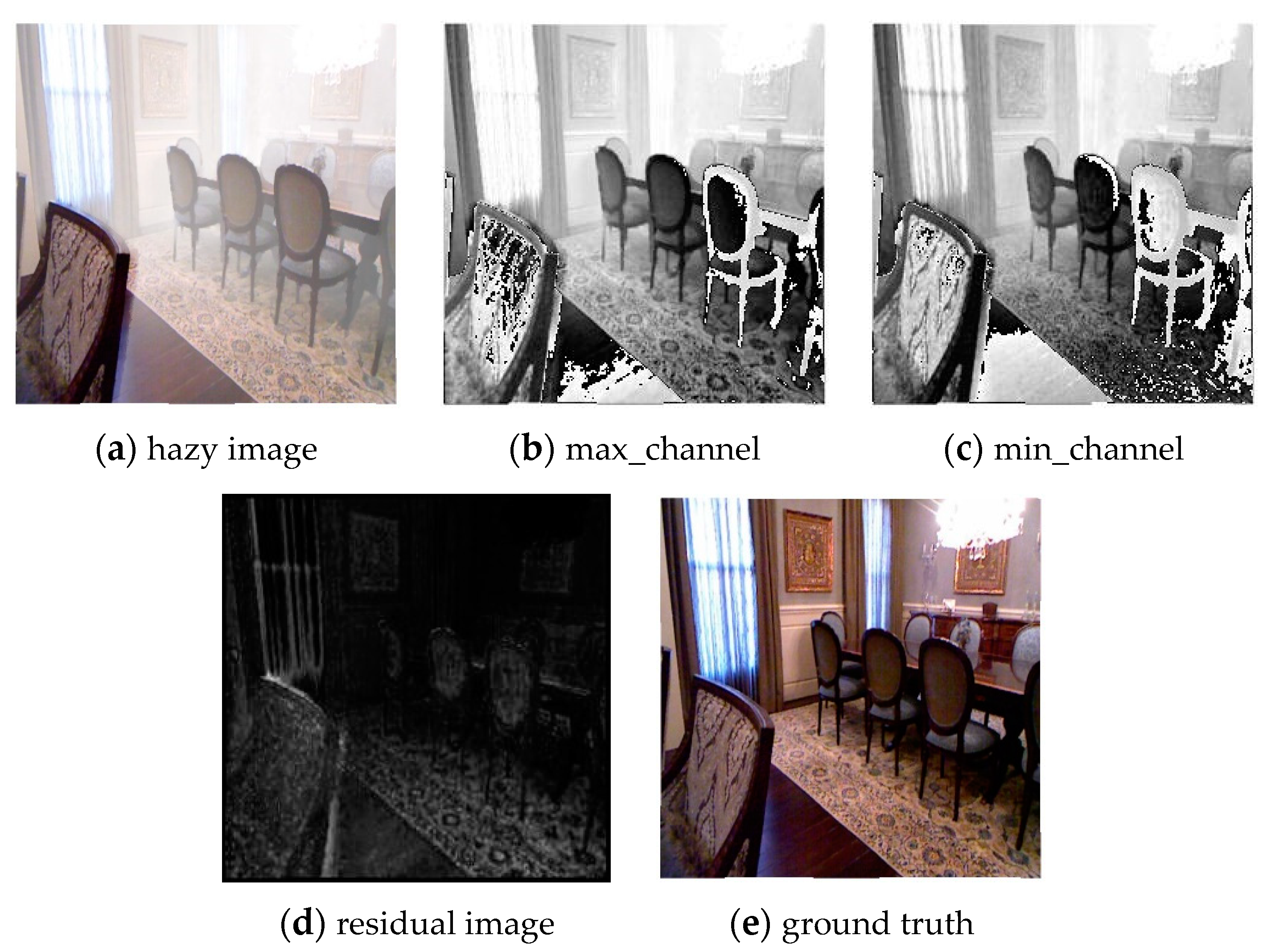
3.1.1. Transfer and Guide Module

In the input hazy image, due to the presence of haze, the recovery of contour information was affected during the entire process of image restoration, often causing a halo-like phenomenon. Therefore, we designed a transfer module to obtain the background of the hazy image, then used the background, as shown in Figure 3, to guide the training of the guide filter layer. We obtained the reference image (called the residual image) by subtracting the minimum channel value from the maximum channel value of each point in the RGB (Red Green Blue) image.
Inspired by [24], we created a separable CNN layer as shown in Figure 4 that could be distinguished during training. Also, we obtained a hazy image with high resolution (IH) and downsampled it to obtain a hazy image of low resolution (IL). Next, we produced a guided image (IR) with our transferring operator. Finally, we fed the three images into the guided filtering layer to obtain the high-frequency component.
The principle of the guided filtering layer is as follows:
I R i = a L k I L i + b L k , i w k
O L = a H I H + b H
where i is the pixel position. Suppose that in the filtering window wk with a radius of r (k is the label of the window), there is a linear relationship shown in Equation (2). aH and bH are obtained by upsampling aL and bL. These parameters are obtained by training the guided filtering layer [24]. Specifically, first send IL into the convolutional layer, then send its output and IR into the mean filter and local linear model (Equation (2)), and get the aL and bL by minimizing the loss of input and output. Therefore, two parameters need to be set before training, i.e., the radius r of the mean filter window (smoothing kernel) and the regularization coefficient ε. Finally, the low-frequency component OL is output by Equation (3). Specifically, we first smoothed the image. Starting with input (IH,IL,IR), the smoothed image was the low-frequency component OL, and we obtained the high-frequency component OH by means of the following subtraction: OH = IH − OL.
The most important thing in this module is that we used the residual image [25] as the guide image to guide the filter in our low-pass smoothing process. Such guided filtering resulted in a small amount of high-frequency information in the low-frequency components. Therefore, only the contour information of the background was included in the high frequency information, which greatly facilitated our subsequent restoration of the contour details.
In order to obtain more details of the contour, as shown in Figure 2, we took some columns of smoothing kernels. In particular, by guiding the filter layer, we connected all the high-frequency components and mapped them to higher dimensions through a feature-mapping channel, providing feature information for subsequent image reconstruction.
The high-frequency components were obtained by setting different smoothing kernels and regularization coefficients, as shown in Figure 5. The main influence on the results was the smoothing kernel. The larger the kernel, the more textures and details it captured, while the regularization coefficient was mainly used to prevent parameters from getting too large. Different smoothing kernels could help us capture more details and may solve the problem regarding the haze concentration, which often changes significantly in different regions of the hazy image.

3.1.2. Generator

Generators are used to generate clear images by retaining the structure and details of the image and eliminating the haze. We adopted the symmetrical encoding and decoding structure of “U-net” [20] and “ResNet” [19]. The encoder was composed of convolutional layers and performed downsampling operations, and the features were mapped to the corresponding layer in the decoding process. The decoder consisted of a convolutional layer and a nonlinear spatial transmission and performed an upsampling operation. In addition, we connected the contour information obtained by the decomposition guidance module with the highest layer of the encoder after implementing the mapping channel, which effectively prevented the global contour information from being affected by the local feature information in the downsampling process, yielding more complete and clear contour features.

3.1.3. Discriminator

The discriminator accepts the output of the generator and determines whether the generated image is a real and clear image. Similar to [26], we designed a neural network, the basic operations of which were convolution, batch normalization and Leaky Rectified Linear Unit (LeakyReLU) activation.

3.2. Enhanced Loss Function with Perceptual Loss

The generator introduces three losses, as shown by Equation (4). Namely, Ladv is the adversarial loss, Lpixel is the pixel loss, Lperceptual is the perceptual loss and μ is the weight of the perceptual loss.
L a l l = L a d v + L p i x + μ L p e r c e p t u a l
where Ladv adopts the adversarial loss of GAN, as in Equation (5). Here, x is the input hazy image, Pdata(x) is the dataset of x, G is the generator and D is the discriminator:
L a d v = E x P d a t a ( x ) [ log ( 1 D ( G ( x ) ) ) ]
The pixel loss was originally used to compute paired image-to-image transfer tasks, but now it is used to compute the L1-Norm between a generated image and a really clear image (ground truth):
L p i x = E x P d a t a ( x ) , y P d a t a ( y ) [ y G ( x ) 1 ]
where y is the ground truth and Pdata(y) is the dataset of y. However, this only computes the loss of a style transfer between the generated image and the really clear image, which is not sufficient to restore all texture information, because most of the hazy images are very blurred. Therefore, we added a perceptual loss function to maintain the original image structure by extracting high-level and low-level feature information from the second and fifth pool layers of the Visual Geometry Group 16 (VGG16) [27] architecture. The expression of the perceptual loss function is as follows:
L p e r c e p t u a l ( y ^ , y ) = 1 C i H i W i ϕ i ( y ^ ) ϕ i ( y ) 2 2 = 1 C 2 H 2 W 2 ϕ 2 ( y ^ ) ϕ 2 ( y ) 2 2 + 1 C 5 H 5 W 5 ϕ 5 ( y ^ ) ϕ 5 ( y ) 2 2
where ( y ^ , y) is a pair of the generated images and the really clear image, i represents the ith layer of VGG16 [27], ϕi( y ^ ) and ϕi(y) are the feature maps of layer i of VGG16 induced by the network output and the really clear image and CiHiWi is the size of the feature map in the ith layer. In this way, we can compare the image in the feature space instead of the image in the pixel space and use the generated image and the really clear image to reconstruct the features in the two spaces for comparison to maintain a higher definition of the image that is similar to the really clear image.

3.3. Training

Training of the GAN module. After the Transfer and Guided modules, we obtained the 10 high-frequency components and concatenated them. Then, according to Algorithm 1, we resized our training data before feeding it into the network and ran the network with 1449 pairs from the training dataset. In each iteration, the high-frequency components (GM) obtained from the guided filter and the encoder output (XE) were concatenated and sent (Xcombination) to the decoder to get the output of the generator. Finally, the generator and discriminator were updated separately.
Algorithm 1 GAN module training
Input:
nb ← the batch size;
n ← epochs of training;
λ ← the hyper-parameter;
 Sample hazy examples X = {X(1),…,X(nb)}
 Sample clear examples Y = {Y(1),…,Y(nb)}
 Resize(X, [256, 256])
 Resize(Y, [256, 256])
for epoch = 0; epoch < epochs do
 Guided map GM = Residual_Guided_Filter(X)
 Encode XXE
 Concat XE, GMXcombination
 Decode Xcombination, the output of generator(G)
 Update generator(G) by descending the gradient of Equation (2)
 Update discriminator(D) by descending the gradient of the sum of MSE(D(Y,X),1) and MSE(D(,X),0)
In order to make the GAN module learn the nonlinear mapping from the hazy image and create a clear image, we recursively feed the output back to the generator once.

4. Experiments and Results

Here, we validate our method using synthetic datasets and real datasets and compare our proposed method with five state-of-the-art methods: DCP [3], DehazeNet [15], AOD-Net [16], cGAN [28] and DCPDN [23]. In addition, ablation studies are carried out to prove the effectiveness of our method.

4.1. Experimental Settings

Dataset. We used the Nyu-depth v2 dataset [29] as our training images. Nyu-depth V2 dataset consists of 1449 pairs of indoor color images with dense markers of ground truth depth information, with sizes of 640 × 480. For each image in the training set, we extract 40 × 40 patches with a stride number of 30, resulting in 466,435 training patches generated in total.
We used three test sets, namely, O-HAZE [30], I-HAZE [31] and SOTS (Synthesis Object Testing Set). I-HAZE and O-HAZE contain 35 and 45 pairs of images consisting of hazy images and clear images (ground truth), where the smoke is produced by a professional haze-generation machine, and SOTS belongs to RESIDE [32], a synthetic outdoor dataset, setting the atmospheric light a of each channel between [0.7, 1.0], and uniformly randomly selecting the beta between [0.6, 1.8].
Training details. We adopted the ADAM optimizer with a batch size of 1. The learning rate was set to 0.0002 and the exponential decay rates were (β1, β2) = (0.5, 0.999). We took μ as 0.001. We implemented our method with PyTorch framework and nvidia 1080 Ti GPU on the ubuntu 16.04 system and used the PyCharm software.
The guided filtering layer. The smoothing filter radii were set to {2, 4, 8, 16, 32}, and the regularization coefficients were set to {0.001, 0.0001}.

4.2. Quality Measures

We used two evaluation indicators to evaluate our method, including the Peak Signal-to-Noise Ratio (PSNR) and the Structural Similarity Index Metric (SSIM). These are common indicators for image quality evaluation. PSNR is generally used for engineering projects between maximum signal and background noise. It is based on the error between the corresponding pixels, expressed as:
P S N R = 10 × log 10 { L 2 M S E }
M S E = 1 m n i = 0 m 1 j = 0 n 1 [ y ( i , j ) x ( i , j ) ] 2
where x represents the generated image, y represents the really clear image and the image size is m × n. MSE represents the mean square error between x and y and L is the dynamic range of the pixel values. The higher the PSNR value, the better the generated image. SSIM is used to evaluate the similarity of two images by using the mean value as the brightness estimation, the standard deviation as the contrast estimation and the covariance as the structure similarity measurement. The SSIM expressed as:
S S I M ( x , y ) = ( 2 μ x μ y + c 1 ) ( 2 σ x y + c 2 ) ( μ x 2 + μ y 2 + c 1 ) ( σ x 2 + σ y 2 + c 2 )
where μx and μy are the averages of x and y, σ x 2 and σ y 2 are the variances of x and y, σxy is the covariance of x and y, c1 = (k1L)2 and c2 = (k2L)2 are the constants used to maintain stability and k1 = 0.01 and k2 = 0.03 are the default values. The value range of SSIM is 0 to 1. The closer the SSIM value is to 1, the more similar the two images are.

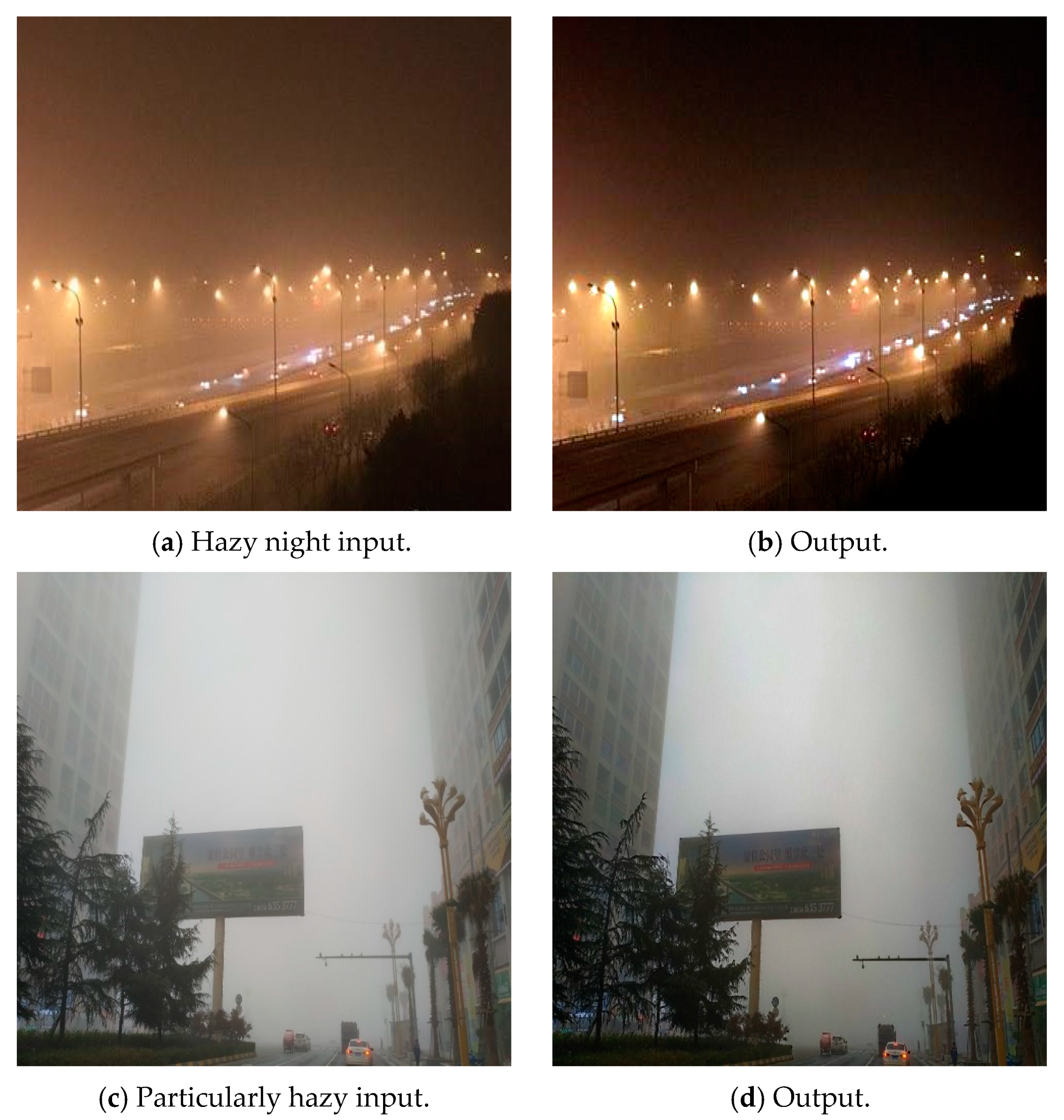
4.3. Comparisions with State-Of-Art Methods

Results of the synthesis dataset. We recorded the results of our method and other advanced methods using the SOTS [32] test set, as shown in Table 1.
For the synthesis dataset of SOTS [32], our network achieved a good performance with respect to both the PSNR and the SSIM. Table 1 demonstrates that our method performed best using the indoor dataset of SOTS, and produced increases of 1.22 dB in the PSNR and 0.01 in the SSIM compared with the second most successful method.
For the outdoor dataset of SOTS, our method achieved the best performance in terms of PSNR and ranked second in terms of SSIM compared with other methods.
In Figure 6, we show three examples of SOTS [32]. All of the methods were shown to be effective on this dataset, but DCP [3] rendered recovered images that were too heavy in color and also generated artifacts in the images, which led to blurriness. AOD-Net [16] brought out deep color, and DehazeNet [15] gave the images high contrast.
O-HAZE and I-HAZE use hazy images generated by a professional haze generating machine. Table 2 shows the results of the average of the PSNR and SSIM values, and we display some sample results in Figure 6.
Results using real-world images. The visual comparison results of the images obtained by these methods using real hazy images can be seen in Figure 7. Several observations can be made: (1) Our method effectively removes the haze of real haze images, even during training on a synthetic dataset, thereby proving the robustness of the method; (2) DCP [4] causes color distortion in the sky area, but our method does not have this problem, instead eliminating the negative effects caused by DCP [4]; and (3) DehazeNet [15] and AOD-Net [16] are poor dehazing methods, whereas DCPDN [23] and cGAN [28] cannot effectively eliminate haze in images with dense fog. The method we propose demonstrates better visual effects.
As shown in Figure 7, DCP cannot properly handle the area of sky in the hazy image, therefore, it is likely to generate artifacts during the dehazing progress, as seen in the 1st, 2nd and 4th images in Figure 7. Also, heavy artifacts exist around the ground in the 7th image in Figure 7. DehazeNet [15] blurs the background in some images, such as in the 3rd, 4th and 6th images in Figure 7. AOD-Net [16] performs well on a synthesis dataset, creating a low brightness image, causing the foreground of these images to fade, as observed in the 7th and 8th images of Figure 7. The colors of the image restored by cGAN and by our method are more distinct than other methods, as shown in Figure 7, but our method is demonstrably better than cGAN in terms of prospective image recovery; our method is more realistic and effective in color and contour restoration.

5. Analysis and Discussion

Here, we analyze and discuss the effect of our method with respect to network architectures and loss functions. We also demonstrate the effectiveness of our proposed method in terms of modules and loss functions by means of an ablation study. Finally, we discuss the limitations of our work.

5.1. Ablation Study

To better demonstrate the effectiveness of the architecture of our method, we conducted an ablation study combining three factors, namely, cGAN, the decomposition guided module (DGM) and the pipeline and perceptual loss (PL). We constructed the following variants with different component combinations: (1) cGAN, where only pix2pix [28] was used; (2) cGAN + DGM, where the results of DM and the hazy image were concatenated to be passed on to pix2pix; (3) cGAN + DM + pipeline, where a pipeline extracted the features of the results of the decomposition guided module; and (4) cGAN + DGM + pipeline + PL, which considered additional perceptual loss to train the network.
We implemented ablation experiments on SOTS [32]; these results are given in Table 3. The results demonstrated that the proposed method achieved the best image dehazing performance compared with pix2pix [28]. PSNR and SSIM improved by 2.71 dB and 0.023, respectively.

5.2. Limitations

The decomposition module of our method was adopted from [24], where we trained a transfer and guided module as an independent CNN layer and our model was trained based on the synthetic dataset. However, the proposed method may be not be able to generate clear images, while the dehazing model is not suitable for hazy images. According to our experiments, our model does not work well for hazy night images or for especially hazy images, probably because our decomposition module cannot effectively extract the high-frequency components of background information in hazy night images and particularly hazy images, as shown in Figure 8.
The following images were collected from the China Weather Net. Our method was shown not to work on hazy night images, possibly because our training dataset did not contain hazy night images, so the GAN module could not learn mapping from a hazy image to a clear image. Future work should involve collecting hazy night images and add them to our existing dataset.
Our method draws a clear distinction between the close-range contours and the foreground profile in the particularly hazy image, but cannot recover objects covered by severe haze.
Another limitation of the network is its processing time, which is also a problem with many existing deep learning methods. The processing time of each image using our method is 0.91 s, which does not reach the level of real-time processing, and tehrefore cannot be applied to software that requires real-time processing.

6. Conclusions

In this paper, we propose a residual image guided cGAN process for single image dehazing which does not rely on estimations of transmission maps or atmospheric light. We regard the problem of image dehazing as a problem of image generation, and directly use convolutional neural network to learn mapping between hazy and clear images. We use the pix2pix network architecture as the infrastructure and decompose the high-frequency components in the residual image of the hazy image through the decomposition module, then combine the results with the output of the encoder to generate a clear image using the decoder. Experimental results show that our method performs well for both synthetic and real-world datasets. However, only natural images are tested; in the future, we will consider improving the method in this article for satellite images.

Author Contributions

Conceptualization, Q.B.; methodology, Q.B., K.M. and J.L.; formal analysis, H.F.; investigation, J.L. and K.M.; resources, J.F.; writing—original draft preparation, Q.B., K.M. and J.L.; writing—review and editing, Q.B., K.M., J.L., H.F. and J.F.; supervision, Q.B. and J.F.; project administration, H.F. and J.F.; All authors have read and agreed to the published version of the manuscript.

Funding

This research received no external funding.

Acknowledgments

This work was supported by Shaanxi International Science and Technology Cooperation and Exchange Program of China (2017KW-010), Scientific Research Project of Shaanxi Education Department of China (15JK1689).

Conflicts of Interest

The authors declare no conflict of interest.

References

  1. Yu, T.H.; Meng, X.; Zhu, M.; Han, M. An Improved Multi-scale Retinex Fog and Haze Image Enhancement Method. In Proceedings of the International Conference on Information System & Artificial Intelligence, Hong Kong, China, 24–26 June 2016. [Google Scholar]
  2. Fattal, R. Single image dehazing. ACM Trans. Graph. 2008, 27. [Google Scholar] [CrossRef]
  3. Narasimhan, S.; Nayar, S. Vision and the Atmosphere. Int. J. Comput. Vis. 2002, 48, 233–254. [Google Scholar] [CrossRef]
  4. He, K.; Sun, J.; Tang, X. Single Image Haze Removal Using Dark Channel Prior; IEEE Computer Society: Washington, DC, USA, 2011. [Google Scholar]
  5. Du, Y.; Li, X. Recursive Deep Residual Learning for Single Image Dehazing. In Proceedings of the 2018 IEEE/CVF Conference on Computer Vision and Pattern Recognition Workshops (CVPRW), Salt Lack City, UT, USA, 18–22 June 2018. [Google Scholar]
  6. Goodfellow, I.; Pouget-Abadie, J.; Mirza, M.; Xu, B.; Warde-Farley, D.; Ozair, S.; Courville, A.; Bengio, Y. Generative Adversarial Networks. In Proceedings of the Advances in Neural Information Processing Systems, Montreal, QC, Canada, 8–13 December 2014; p. 3. [Google Scholar]
  7. Gibson, K.B.; Vo, D.T.; Nguyen, T.Q. An Investigation of Dehazing Effects on Image and Video Coding. IEEE Trans. Image Process. 2012, 21, 662–673. [Google Scholar] [CrossRef] [PubMed]
  8. Dong, J.; Han, Z.; Zhao, Y.; Wang, W.; Prochazka, A.; Chambers, J. Sparse analysis model based multiplicative noise removal with enhanced regularization. Signal Process. 2017, 137, 160–176. [Google Scholar] [CrossRef] [Green Version]
  9. Wierzbicki, D.; Kedzierski, M.; Grochala, A. A Method for Dehazing Images Obtained from Low Altitudes during High-Pressure Fronts. Remote Sens. 2020, 12, 25. [Google Scholar] [CrossRef] [Green Version]
  10. Nishino, K.; Kratz, L.; Lombardi, S. Bayesian Defogging. Int. J. Comput. Vis. 2011, 98. [Google Scholar] [CrossRef]
  11. Zhu, Q.; Mai, J.; Shao, L. A Fast Single Image Haze Removal Algorithm Using Color Attenuation Prior. IEEE Trans. Image Process. 2015, 24, 3522–3533. [Google Scholar]
  12. Meng, G.; Wang, Y.; Duan, J.; Xiang, S.; Pan, C. Efficient Image Dehazing with Boundary Constraint and Contextual Regularization. In Proceedings of the IEEE International Conference on Computer Vision, Sydney, Australia, 1–8 December 2013. [Google Scholar]
  13. Berman, D.; Treibitz, T.; Avidan, S. Non-local Image Dehazing. In Proceedings of the 2016 IEEE Conference on Computer Vision and Pattern Recognition (CVPR), Las Vegas, NV, USA, 27–30 June 2016. [Google Scholar]
  14. Ren, W.; Liu, S.; Zhang, H.; Pan, J.; Cao, X.; Yang, M.H. Single Image Dehazing via Multi-Scale Convolutional Neural Networks; Springer International Publishing: Charm, Switzerland, 2016. [Google Scholar]
  15. Cai, B.; Xu, X.; Jia, K.; Qing, C.; Tao, D. DehazeNet: An End-to-End System for Single Image Haze Removal. IEEE Trans. Image Process. 2016, 25, 5187–5198. [Google Scholar] [CrossRef] [PubMed] [Green Version]
  16. Li, B.; Peng, X.; Wang, Z.; Xu, J.; Feng, D. AOD-Net: All-in-One Dehazing Network. In Proceedings of the 2017 IEEE International Conference on Computer Vision (ICCV), Venice, Italy, 22–29 October 2017. [Google Scholar]
  17. Ren, W.; Ma, L.; Zhang, J.; Pan, J.; Cao, X.; Liu, W.; Yang, M.-H. Gated Fusion Network for Single Image Dehazing. arXiv 2018, arXiv:1804.00213. [Google Scholar]
  18. Li, R.; Pan, J.; Li, Z.; Tang, J. Single Image Dehazing via Conditional Generative Adversarial Network. In Proceedings of the IEEE Conference on Computer Vision and Pattern Recognition (CVPR), Salt Lake City, UT, USA, 18–22 June 2018; pp. 8202–8211. [Google Scholar]
  19. He, K.; Zhang, X.; Ren, S.; Sun, J. Deep Residual Learning for Image Recognition. In Proceedings of the IEEE Conference on Computer Vision & Pattern Recognition, Las Vegas, NV, USA, 27–30 June 2016. [Google Scholar]
  20. Ronneberger, O.; Fischer, P.; Brox, T. U-Net: Convolutional Networks for Biomedical Image Segmentation. In Proceedings of the International Conference on Medical Image Computing and Computer-Assisted Intervention, Munich, Germany, 5–9 October 2015. [Google Scholar]
  21. Engin, D.; Genç, A.; Kemal Ekenel, H. Cycle-Dehaze: Enhanced CycleGAN for Single Image Dehazing. arXiv 2018, arXiv:1805.05308. [Google Scholar]
  22. Du, Y.; Li, X. Perceptually Optimized Generative Adversarial Network for Single Image Dehazing. arXiv 2018, arXiv:1805.01084. [Google Scholar]
  23. Zhang, H.; Patel, V.M. Densely Connected Pyramid Dehazing Network. In Proceedings of the 2018 IEEE/CVF Conference on Computer Vision and Pattern Recognition, Las Vegas, NV, USA, 18–23 June 2018. [Google Scholar]
  24. Wu, H.; Zheng, S.; Zhang, J.; Huang, K. Fast End-to-End Trainable Guided Filter. In Proceedings of the 2018 IEEE/CVF Conference on Computer Vision and Pattern Recognition, Las Vegas, NV, USA, 18–23 June 2018; pp. 1838–1847. [Google Scholar]
  25. Li, R.; Tan, R.T.; Cheong, L.-F. Robust Optical Flow Estimation in Rainy Scenes. arXiv 2017, arXiv:1704.05239. [Google Scholar]
  26. Zhang, H.; Sindagi, V.; Patel, V.M. Image De-raining Using a Conditional Generative Adversarial Network. IEEE Trans. Circuits Syst. Video Technol. 2019, 1. [Google Scholar] [CrossRef] [Green Version]
  27. Simonyan, K.; Zisserman, A. Very Deep Convolutional Networks for Large-Scale Image Recognition. arXiv 2014, arXiv:1409.1556. [Google Scholar]
  28. Sohn, K.; Yan, X.; Lee, H.; Arbor, A. Learning Structured Output Representation using Deep Conditional Generative Models. In Proceedings of the International Conference on Neural Information Processing Systems, Montreal, QC, Canada, 7–12 December 2015. [Google Scholar]
  29. Silberman, N.; Hoiem, D.; Kohli, P.; Fergus, R. Indoor Segmentation and Support Inference from RGBD Images. In Proceedings of the 12th European conference on Computer Vision—Volume Part V, Florence, Italy, 7–13 October 2012. [Google Scholar]
  30. Ancuti, C.O.; Ancuti, C.; Timofte, R.; De Vleeschouwer, C. O-HAZE: A dehazing benchmark with real hazy and haze-free outdoor images. arXiv 2018, arXiv:1804.05101. [Google Scholar]
  31. Ancuti, C.O.; Ancuti, C.; Timofte, R.; De Vleeschouwer, C. I-HAZE: A dehazing benchmark with real hazy and haze-free indoor images. arXiv 2018, arXiv:1804.05091. [Google Scholar]
  32. Li, B.; Ren, W.; Fu, D.; Tao, D.; Feng, D.; Zeng, W.; Wang, Z. Benchmarking Single Image Dehazing and Beyond. arXiv 2017, arXiv:1712.04143. [Google Scholar] [CrossRef] [PubMed] [Green Version]
Figure 1. Image dehazing examples with and without prior information. (a) Input hazy image; (b) dark channel prior (DCP); (c) ours; (d) ground truth.
Applsci 10 05898 g001
Figure 2. The architecture of the entire network.
Applsci 10 05898 g002
Figure 3. Intermediate results of the decomposition process.
Applsci 10 05898 g003
Figure 4. Intermediate results of the decomposition process.
Applsci 10 05898 g004
Figure 5. Frequency components after different filtering parameters.
Applsci 10 05898 g005
Figure 6. Comparison of state-of-the-art dehazing methods using synthesis images.
Applsci 10 05898 g006
Figure 7. Dehazing results for a real-world dataset.
Applsci 10 05898 g007
Figure 8. The results of our method on a hazy night image and on a particularly hazy image.
Applsci 10 05898 g008
Table 1. Average Peak Signal-to-Noise ratio (PSNR) and Structural Similarity Index Metric (SSIM) results on SOTS (Synthesis Object Testing Set). (red font indicates the highest value, followed by blue font).
MethodDCPDehazeNetAOD-NetcGANDCPDNOurs
IndoorPSNR18.0522.3619.7821.0218.2223.58
SSIM0.8170.8440.8870.8390.8150.897
OutdoorPSNR18.7422.5721.1220.3519.9523.06
SSIM0.8230.8520.8970.8550.8420.878
DCP: Dark Channel Prior; AOD-Net: ALL-in-One Dehazing Network; cGAN: Conditional Generative Adversarial Network; DCPDN: Densely Connected Pyramid Dehazing Network.
Table 2. Average PSNR and SSIM results of O-HAZE and I-HAZE. (red font indicates the highest value, followed by blue font).
MethodDCPDehazeNetAOD-NetcGANDCPDNOurs
O-HAZE [28]PSNR13.5316.9317.8717.3716.2317.49
SSIM0.6390.6740.6360.6350.6110.679
I-HAZE [29]PSNR14.2416.7018.5317.4817.0918.57
SSIM0.7610.7870.8400.8030.8370.827
Table 3. Quantitative evaluation of the effects of different components in the outdoors.
CombinationPSNRSSIM
cGAN20.350.855
cGAN + DM22.030.869
cGAN + DM + pipeline22.950.867
cGAN + DM + pipeline + PL(ours)23.060.878

