Article

On the Matricial Formulation of Iterative Sweep Power Flow for Radial and Meshed Distribution Networks with Guarantee of Convergence

by
Oscar Danilo Montoya
1,2,*,
Walter Gil-González
3 and
Diego Armando Giral
4
1
Facultad de Ingeniería, Universidad Distrital Francisco José de Caldas, Bogotá D.C. 11021, Colombia
2
Laboratorio Inteligente de Energía, Universidad Tecnológica de Bolívar, Cartagena 131001, Colombia
3
Grupo GIIEN, Facultad de Ingeniería, Institución Universitaria Pascual Bravo, Campus Robledo, Medellín 050036, Colombia
4
Facultad Tecnológica, Universidad Distrital Francisco José de Caldas, Bogotá D.C. 11021, Colombia
*
Author to whom correspondence should be addressed.
Appl. Sci. 2020, 10(17), 5802; https://doi.org/10.3390/app10175802
Submission received: 1 August 2020 / Revised: 14 August 2020 / Accepted: 18 August 2020 / Published: 21 August 2020
(This article belongs to the Section Electrical, Electronics and Communications Engineering)

Abstract

:
This paper presents a general formulation of the classical iterative-sweep power flow, which is widely known as the backward–forward method. This formulation is performed by a branch-to-node incidence matrix with the main advantage that this approach can be used with radial and meshed configurations. The convergence test is performed using the Banach fixed-point theorem while considering the dominant diagonal structure of the demand-to-demand admittance matrix. A numerical example is presented in tutorial form using the MATLAB interface, which aids beginners in understanding the basic concepts of power-flow programming in distribution system analysis. Two classical test feeders comprising 33 and 69 nodes are used to validate the proposed formulation in comparison with conventional methods such as the Gauss–Seidel and Newton–Raphson power-flow formulations.

1. Introduction

1.1. General Context

Electrical distribution networks represent the most significant portion of the power system and are entrusted with providing electricity to end-users at medium- and low-voltage levels by connecting the transmission/sub-transmission system with consumers [1,2]. Typical voltages in these electrical networks oscillate between 4.16 kV and 33 kV [3], and these networks are typically operated with a radial structure to minimize installation, operation, and maintenance costs, including protective devices coordination simplifications [4,5,6]. To determine the behavior of electrical networks under well-defined voltage conditions, power flow methodologies are used, which facilitate the calculation of the voltage profiles at all the nodes of the network for a particular load condition [7,8]. The main challenge in the power-flow analysis of distribution networks is the constant power loads that produce nonlinear relationships between the voltages and powers [9,10], which makes the use of numerical methods for solving the power-flow problem necessary [11]. A typical tendency in the power-flow analysis of electrical distribution networks is the use of graph-based methods to address the power-flow problem based on the radial structure of the grid [12,13]. However, these methodologies are not useful in the case of weakly or strongly meshed distribution networks [14], which can cause major issues in modern power systems where meshed structures can help with grid performance in terms of realizing lower power losses and improvement voltage profiles [15]. In the case of commercial solutions for a distribution system analysis such as the DigSILENT and ETAP software, the Newton–Raphson (NR) method is the most-used approach [16] as it can be used with radial and meshed structures as well as multiple slack and voltage-controlled nodes [17]. In this research, we tackle the power-flow problem in electrical distribution networks while considering a unique slack node and radial and meshed configurations by reformulating the conventional backward–forward power flow using the branch-to-nodal admittance matrix [18].

1.2. Motivation

The power-flow analysis in electrical distribution networks is one of the most classical and largely studied problems in power-system analysis [14] as the power-flow is a necessary calculation in the determination of grid performance [10]. A power-flow method is a tool that is used to determine, via an iterative procedure, the final values of all the voltages in an electrical network with a certain tolerance acceptance in order to determine the complete operative state [14], i.e., currents through lines, voltage regulation in all the nodes, active and reactive power losses, and voltage stability. To solve the power-flow problem, the most classical methods used are the NR and Gauss–Seidel (GS) approaches, which guarantee convergence based on the Kantarovich and Banach fixed-point theorems [19]. In addition, some graph-based methods such as triangular formulation and quasi-symmetric matrices have also been reported for handling radial grid configurations [12,20]. However, this research is motivated by the fact that the classical backward–forward power-flow method is commonly formulated via sequential steps that require that the grid is ordered in layers [21]. It has a radial structure as, all the currents are calculated in the backward stage, while all the voltages are defined in the forward stage [13]. As this operation can be efficient, these stages exclude meshed configurations, which implies that it is not applicable to weakly or strongly meshed distribution networks. Therefore, herein, a reformulation of the backward–forward power flow in distribution networks is presented based on the branch-to-nodal incidence matrix [13], which permits the handling of radial and meshed distribution networks that include voltage-controlled nodes. Furthermore, the convergence of the proposed method is demonstrated by applying the Banach fixed-point theorem [22].

1.3. Literature Review

Power-flow solutions in the literature present a vast universe of possibilities based on iterative procedures, linearization methods, and convex reformulations. Some of these approaches are presented below.
The most classical power-flow methods in power-systems analysis correspond to the Gauss-Seidel (GS) and NR approaches [14]. The GS approach can be easily implemented using any programming language with its main advantage being that it can be used with complex numbers. However, it exhibits the worse performance in terms of processing time and number of iterations. With the purpose of improving the efficiency of the GS method, an accelerating factor α that reduces the total number of iterations and the required overall processing time is used [17]. In the case of the NR approach, it is a methodology that is more commonly used in commercial software and is widely adopted by utilities [23]. The main advantage of the NR approach is that it converges in a few iterations, has low processing times, and can possibly be used with radial and meshed networks comprising multiple voltage-controlled nodes. The main problem with using the NR approach in distribution networks is the high dispersion of the Jacobian matrix, which may cause convergence problems when the matrix is inverted for updating the voltage magnitude and angle variables [19]. The authors of [24] proposed the use of the Levenberg–Marquardt (LM) algorithm for solving power-flow problems in electrical networks; this approach essentially comprises an alternative manner of presenting the NR formulation with the main advantage that a factor is added to the Jacobian in order to reduce the possible singularities in this matrix.
For distribution networks, some of the most recognized approaches for addressing the power-flow problem are graph-based methodologies known as backward–forward and triangular methods [12,20]. The backward–forward method is typically designed with an algorithmic structure using an iterative sweep based on currents in the backward stage to update the voltages in the forward stage [21]. An important improvement in the backward–forward approach was presented by [13], wherein radial and meshed structures were included in a matricial formulation. The triangular approach works for radial and meshed structures [12]; however, the related convergence analysis is not provided. It should be noted that in these methods, the authors do not present an analysis of the inclusion of voltage-controlled nodes, which we proposed in our matricial reformulation. A new approach based on successive approximations was recently reported in [
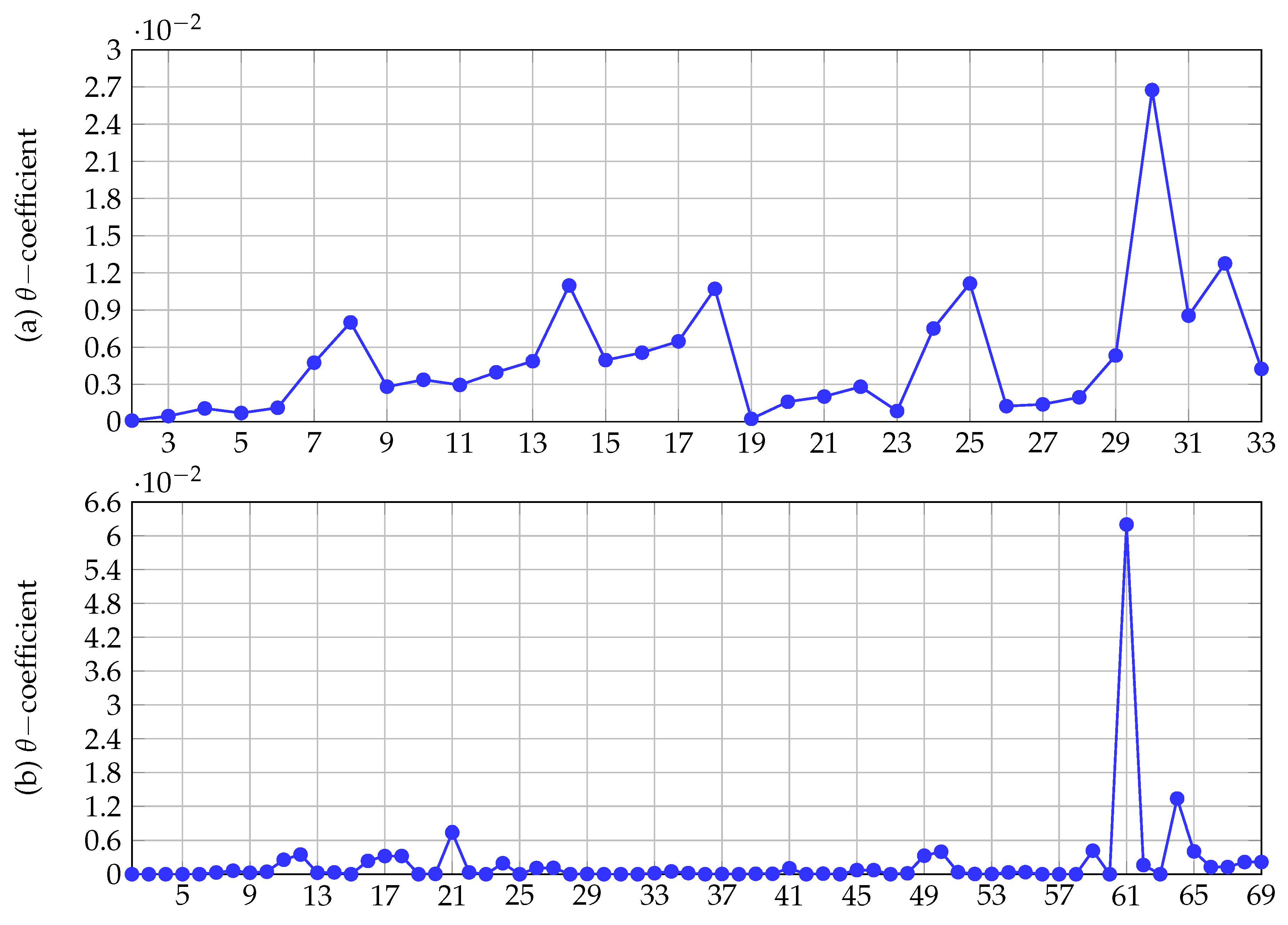
25]. This approach demonstrates the convergence of the recursive formulation for radial and meshed networks using the Banach fixed-point theorem. However, voltage-controlled sources were not considered in this formulation, and the behavior of the θ -coefficient was not determined to confirm the convergence at well-defined voltage conditions. Two additional important power flow contributions have been reported in specialized literature by [26,27] regarding secondary distribution networks to study the problem of the harmonic penetration caused by higher penetration of photovoltaic sources. The authors in these approaches have proposed a harmonic power flow analysis using affine arithmetic which allows reaching better results regarding harmonic distortion estimations with low-computational effort when compared with classical Monte-Carlo simulations; in addition, these methods were validate in real secondary distribution networks with promissory results for utilities.
Other approaches have also been presented in specialized literature in relation to linear and convex approximations for power-flow solutions in distribution networks. In [11], a convex approximation for a power-flow analysis of radial and meshed distribution networks was presented while considering a semidefinite programming approximation by using a rectangular representation of the power-balance equations. In [8], a second-order cone programming approximation was described while considering branch variables related to currents and powers in all the lines. It is essential to mention that the main disadvantage of these approaches is the low rate of convergence when the number of nodes (n) increases as these formulations create n 2 variables related to voltages, which increase the required processing times to reach the optimal solution in the iterative procedure [28]. In the case of linear methodologies, the authors of [7] proposed a Taylor’s series expansion of the hyperbolic relation between the voltage and powers to reach a linear formulation that can be used to solve directly without the use of iterative procedures. In [10], an improvement of this linear approximation was presented using the straight equation to include the minimum expected voltage in the approximation and improve the final result of the power-loss calculation. The authors of [29] described a linear approximation based on a logarithmic transformation of the voltage magnitudes added to the Taylor’s series expansion for applications in power systems. It should be noted that these linear approximations have speed responses; however, the final result of the power-loss estimation varies in the range of 1% and 10%.

1.4. Contributions and Scope

The main contributions of this research can be summarized as follows:
  • The reformulation of the classical backward–forward power-flow method for application to distribution networks with the ability to handle radial and meshed configurations by rewriting the branch variables into nodal variables using the branch-to-node incidence matrix.
  • The parametric independence of the power-flow formulation, as no assumptions about relations reactance/resistance, are required in the proposed matricial formulation.
  • The possibility of guaranteeing convergence under well-defined voltage conditions by applying the Banach fixed-point theorem to the recursive solution, which only requires that the short-circuit current be more significant to the load current in all the nodes to ensure the convergence of the algorithm.
  • The presentation of the proposed matricial formulation in an intuitive manner to introduce students of electrical engineering to power-flow analysis by providing the MATLAB/OCTAVE algorithm for solving a small test feeder as a numerical example comprising radial and meshed structures.
It is important to mention that a similar approach was previously proposed in [13] that combined branch-to-nodal matrices with triangular matrices; moreover, its convergences were also proved. However, the authors of [13] did not present the behavior of the θ -coefficient as a function of the load current and the short-circuit current relations per node. In addition, a simulation case is presented herein, where the power system contains a voltage-controlled node (VC node) in a small transmission network, which demonstrates that the proposed matricial approach is extensible to power system applications with multiple meshes and VC nodes.

1.5. Organization of the Document

The remainder of this paper is arranged as follows. 
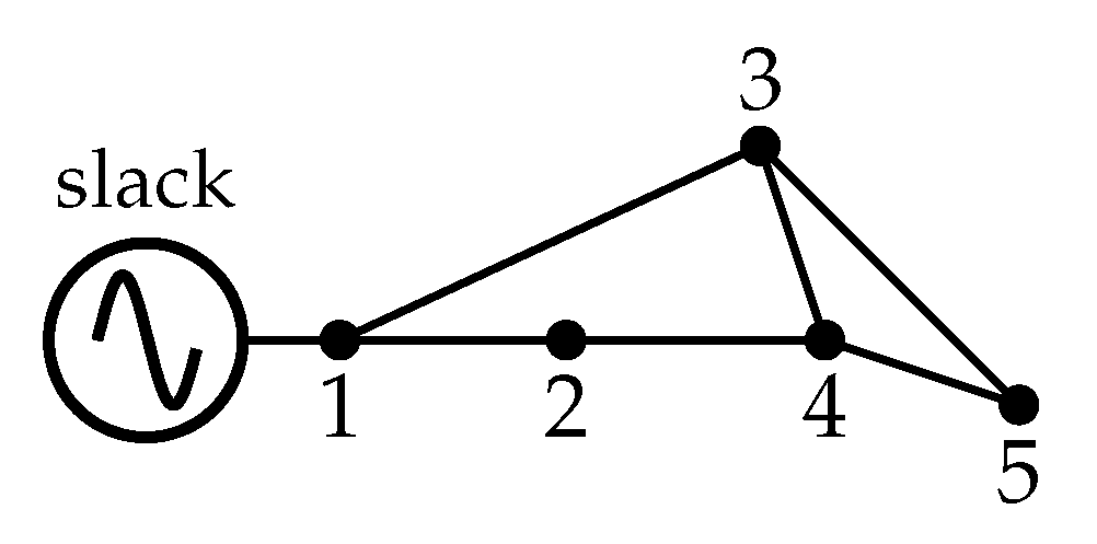
Section 2 presents the matricial formulation of the classical backward–forward power flow method using a small distribution test feeder with multiple meshes. In Section 3, the convergence analysis is presented based on the Banach fixed-point theorem, which results in the maximum load current divided by the minimum short-circuit current per node. 
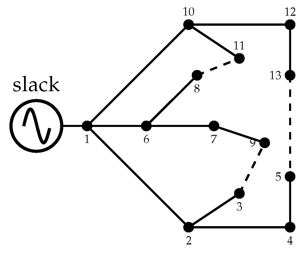
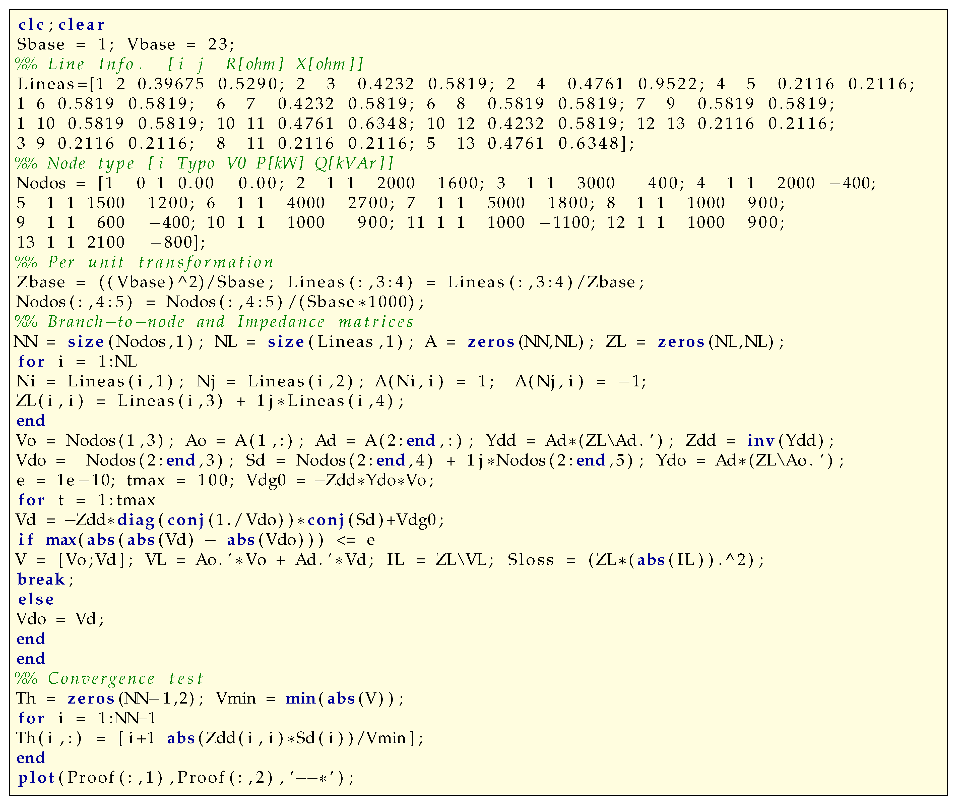
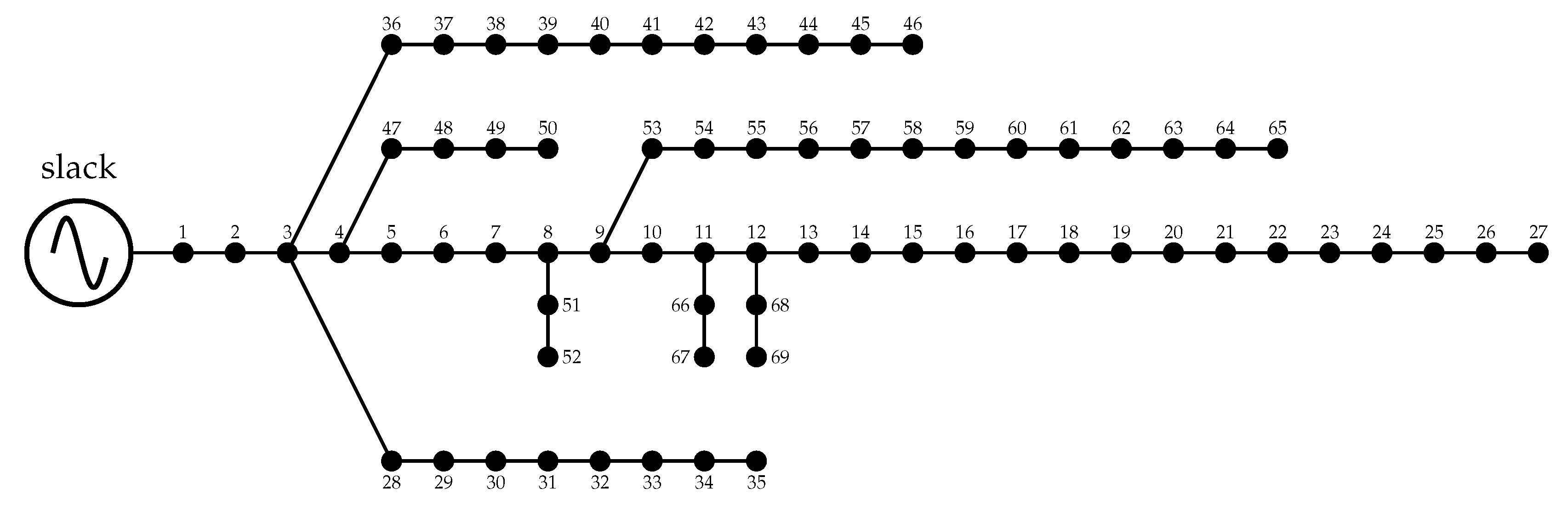
Section 4 presents a small numerical example comprising a 13-node test feeder with mesh and radial topologies and presents the MATLAB/OCTAVE implementation that can be used as a power-flow analysis tutorial for beginners. In 
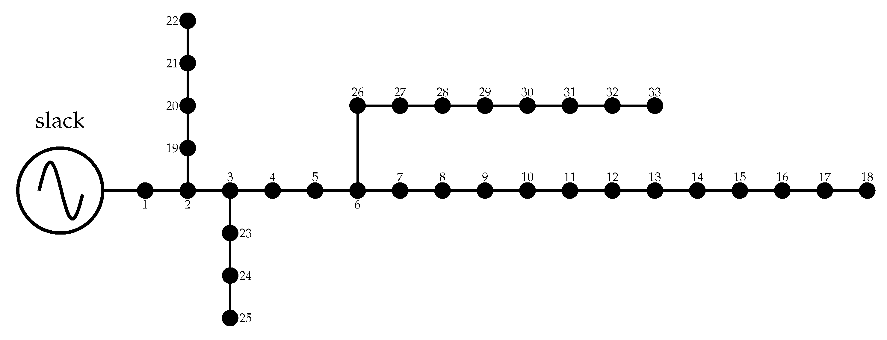
Section 4, the configurations of two classical distribution test feeders comprising 33 and 69 nodes are presented. 
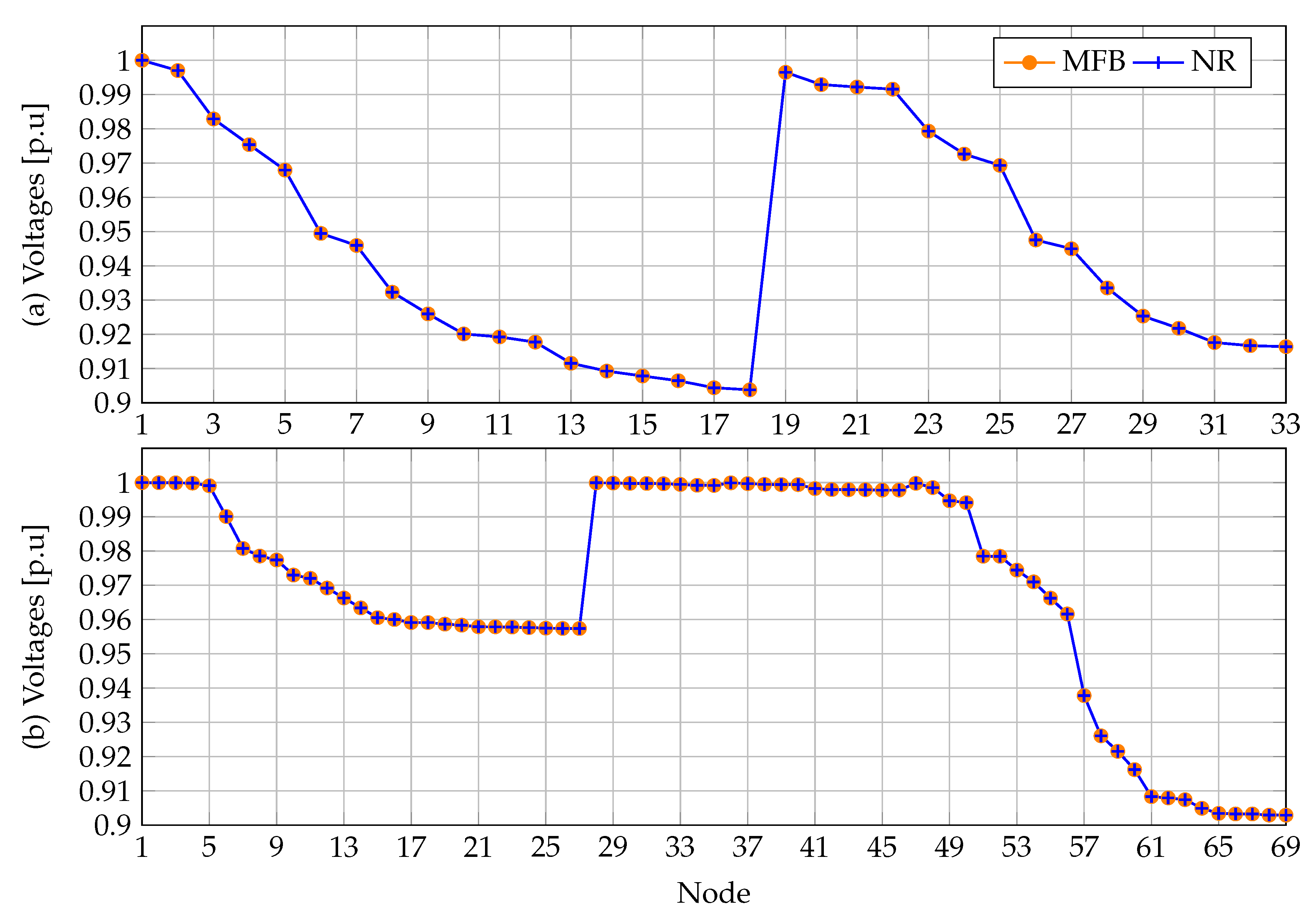
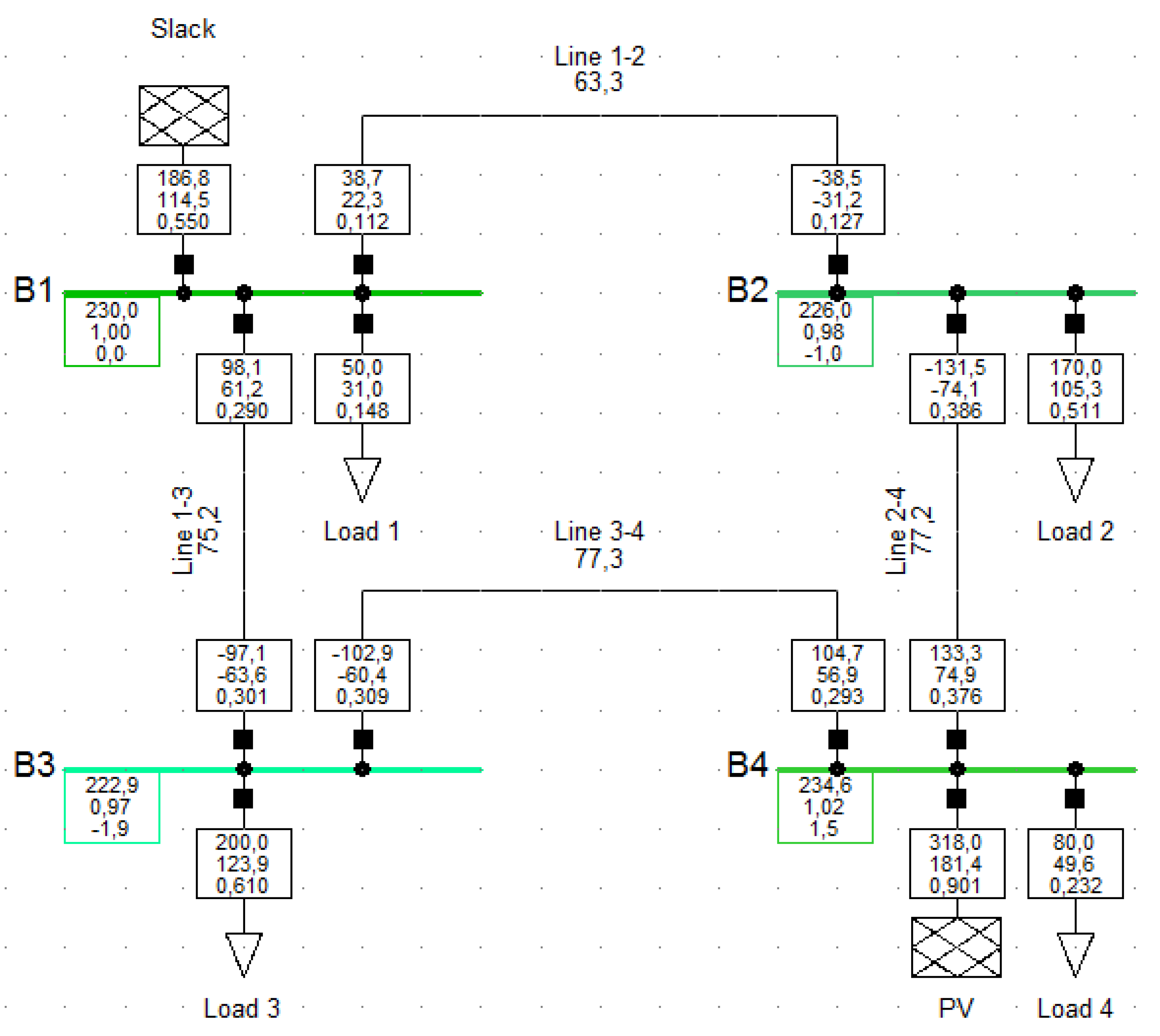
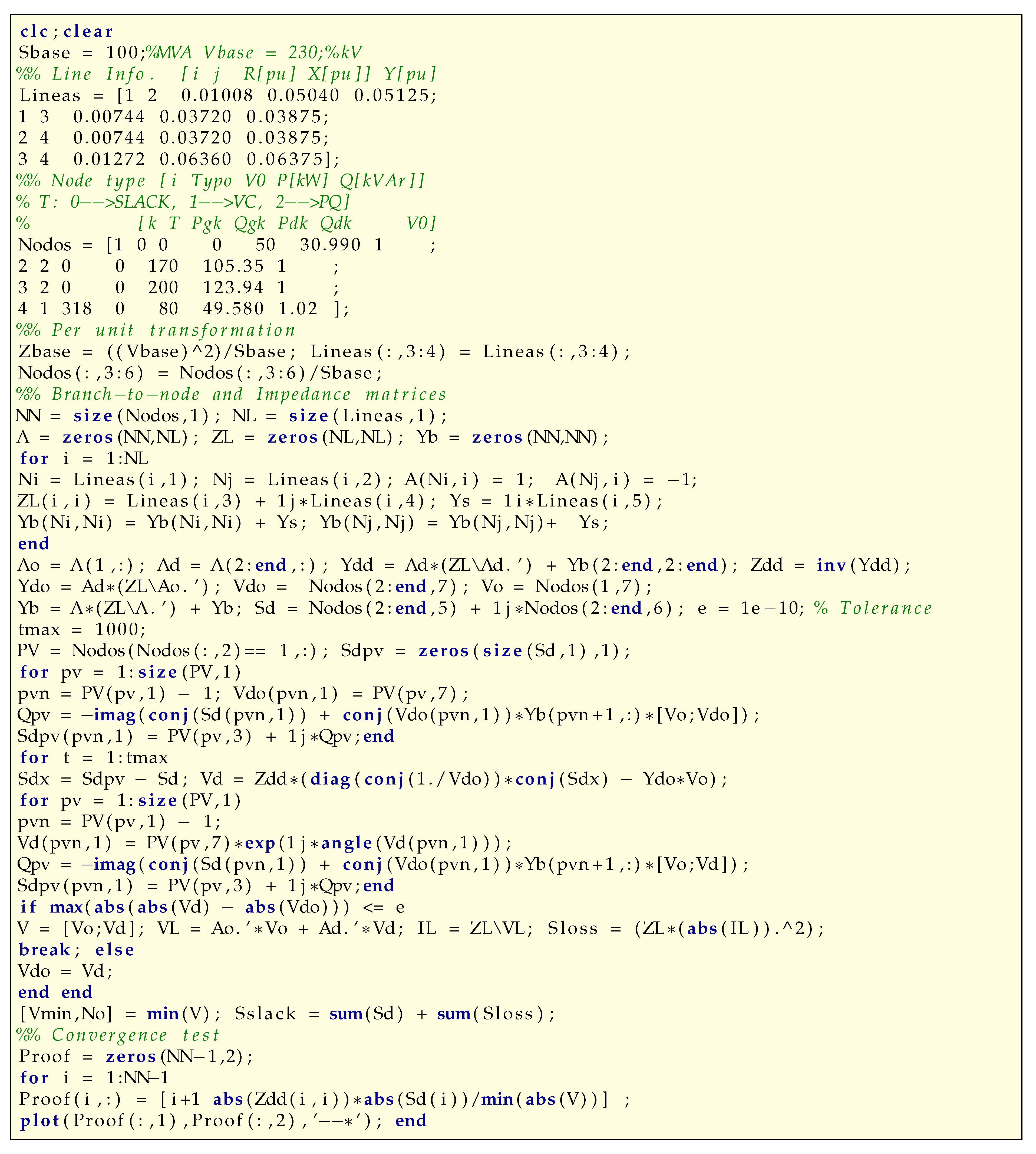
Section 6 presents the numerical results obtained for these test feeders on comparing the proposed matricial formulation with the classical power- flow methods such as the GS, NR, and LM methods; in addition, a small transmission network comprising four nodes that comprise a meshed structure with a voltage-controlled node is presented, which aids in understanding the extension of the proposed formulation to power-system analyses. Section 7 presents the main conclusions derived from this work as well as its possible future improvements.

2. Matricial Power-Flow Formulation

The classical backward–forward power-flow method was developed using the concept of iterative sweeps, which achieves the following [30]:
  • Calculates the total current demands at all the loads with assumed known voltages.
  • Determines all the currents that flow in all the branches of the network by applying the first Kirchhoff’s law at each node.
  • Calculates the voltage drops by starting from the source and using an ordering stage that defines the layers at which nodes are located.
  • Updates the voltage profile in all the demand nodes and repeats all the stages until the convergence tolerance is reached.
This structure of the backward–forward method has two main disadvantages: (i) It can only handle radial grid configurations, and (ii) it requires nodal ordering in layers [20]. However, to address these problems, it is possible to reformulate a power-flow problem using branch-to-nodal incidence matrices [18].
Definition 1
(Branch-to-node incidence matrix A ). An electrical network that is represented by a connected graph with b links and n vertices can be represented by a rectangular matrix A R b × n by assuming arbitrary directions in the current flow through the lines as follows:
  • A i , j = 1 if the line i is connected to the node j and its current leaves from this node.
  • A i , j = 1 if the line i is connected to the node j and its current arrives at this node.
  • A i , j = 0 if the line i is not connected to the node j.
To exemplify the structure of the branch-to-node incidence matrix A , let us consider the electrical network depicted in Figure 1. This grid comprises six links (branches) and five nodes. The names of the lines are listed in Table 1.
On considering the branch information reported in Table 1 and the electrical-grid configuration depicted in Figure 1, the branch-to-node matrix A can take the following form:
A = 1 1 0 0 0 1 0 1 0 0 0 1 0 1 0 0 0 1 1 0 0 0 1 0 1 0 0 0 1 1
It should be noted that this matrix can be split into two sub-matrices that are related to the slack source and the rest of the nodes as follows (This is made possible by assuming the slack node is located at node 1.):
A = A s A d ,
where A s is the first column of A (slack node), and A d corresponds to the rest of the columns in A , i.e., the demand nodes.
Now, let us define the voltage drop at line i as E i and the voltages at its terminals as V j . Then, from Figure 1, we know that
E 1 = V 1 V 2 , E 2 = V 1 V 3 , E 3 = V 2 V 3 , E 4 = V 2 V 4 , E 5 = V 3 V 4 , E 6 = V 4 V 5 ,
which can be rewritten using (1) and (2) as presented below:
E = A s V s + A d V d ,
where V s = V 1 , E is a vector that comprises all the voltage drops, and V d is a vector that comprises all the voltages in the demand nodes.
To relate the currents J in all the branches with the voltage drops, it is possible to apply Ohm’s law as presented below:
E = Z J ,
where Z = diag ( Z 1 , Z 2 , , Z b ) .
To determine the relation between the currents injected at the nodes (i.e., I) and all the branch currents, let us apply Kirchhoff’s second law at each node while considering the current directions defined in Table 1. We thus obtain
I 1 = J 1 + J 2 , I 2 = J 1 + J 3 , I 3 = J 2 + J 4 + J 5 , I 4 = J 3 J 4 + J 6 , I 5 = J 5 J 6 .
It should be noted that I can also be split as
I = I s I d T ,
where I s and I d are the current of generators and demands, respectively.
Using the relation between the branch and nodal currents presented above, it is possible to find that
I s = A s T J ,
I d = A d T J .
Now if expressions (3), (4), and (7) are combined based on Y = Z 1 , then the following result is obtained:
I d = A d T Y A s V s + A d T Y A d V d ,
To find the relation between the injected currents and powers, it is possible to apply the Tellegen’s theorem, which defines apparent power as follows:
I s = diag 1 V s S s ,
I s = diag 1 V d S d .
where the superscript represents the conjugate operator, S s is the apparent power generation in the slack node, and S d are the apparent power consumption in the demand nodes.
Now, if expressions (8) and (10) are combined to obtain V d , the following result is obtained:
V d = Z d d diag 1 V d S d b ,
where Z d d is defined as A d T Y A d 1 , and b = + Z d d A d T Y A s V s .
It should be noted that to solve expression (11), an iterative procedure is required, as this expression has a recursive structure. For this purpose, let us to add an iterative counter t that starts from the initial point t = 0 (i.e., V d 0 is perfectly known), which allows the rewriting of (11) as presented below:
V d t + 1 = Z d d diag 1 V d t , S d b .
Remark 1.
The iterative procedure in (12) is performed until the convergence error ϵ is reached, i.e., max V d t + 1 V d t ϵ or the total number of iterations t max is completed.

3. Convergence Analysis

To prove that the recursive formula (12) guarantees the convergence of the power-flow problem in the case of distribution networks comprising radial and mesh structures formulated using branch-to-nodal incidence matrices, let us consider the following.
Assumption 1.
The amount of power consumed by the loads does produce voltage instabilities in the distribution network, i.e., the system operates under well-defined voltage conditions.
Assumption 2.
There exists a positive lower bound for all the voltage profiles, i.e., V min > 0 , which is typically defined by the utility and regulatory policies.
Assumption 3.
The demand-to-demand impedance matrix, i.e., Z d d , is diagonal dominant, which implies that, always, Z d d j j Z d d j k , j k .
To demonstrate the convergence properties of the recursive power flow approach defined by (12), let us present the general definition of the Banach fixed-point theorem as follows.
Theorem 1
(Banach fixed-point theorem). The iterative formula presented in (12) is stable and corresponds to a contraction map with the form
V d t + 1 = g V d t ,
for some V that fulfills Assumption 1 irrespective of the starting point, i.e., V 0 , such that
g V d 0 g W θ V 0 W
where W is the solution of the power-flow problem, and θ is a real number between 0 and 1.
Proof. 
The recursive formula for the iterative backward–forward power-flow method presented in (12) can be rewritten as follows:
V d t + 1 = g V d t = b Z d d S d i V d i t , i Ω S T
where Ω S is the set that contains all the demand nodes.
In addition, based on the structure of the Banach fixed-point theorem, it is possible to affirm that the solution of the power-flow problem, i.e., W , satisfies W = g W , and it is unique if and only if g W is a contraction mapping on V d .
V d t + 1 W = g V d t + 1 g W Z d d S d 1 W i 1 V d i t , i Ω S T Z d d S d V d i t , W i W i V d i t , i Ω S T θ V d t W ,
where
θ = Z d d S d V min 2 .
Now, on considering Assumption 2, which is regarding the positive definiteness of the impedance matrix, the expression (17) can be reduced to
θ = max i Ω S Z d d i i S d i V min 2 .
It should be noted that, considering the mathematical structure presented in (18) and that Z d d i i is the equivalent impedance at node i, the following relation can be obtained.
θ = max i Ω S S d i V min V min Z d d i i ,
where we can ensure that 0 θ 1 , as the denominator in (19) corresponds to the minimum short-circuit current, and the numerator represents the maximum load current, which is always lower than any short-circuit current during normal operative conditions. This implies that the recursive matricial sweep power flow (12) converges to the power-flow solution, which completes the proof.  □

4. Numerical Example

This section presents a small test feeder comprising 13 nodes that can handle radial or mesh configurations. This facilitates the demonstration of the convergence of the proposed matricial reformulation of the classical backward—forward power flow approach. Figure 2 presents the electrical configuration of the 13-node test feeder.
Table 2 lists the branch and load information for the 13-node test feeder that has a total demand of active and reactive power of 24,200 kW and 7700 kVAr, respectively, and it operates on a line-to-neutral voltage of 23 kV.
To solve the power-flow problem in the 13-node test feeder, we consider the following: (i) a radial configuration is reached when all the dashed lines in Figure 2 are open, and a meshed configuration is obtained when one or more dashed lines are connected; (ii) the recursive formula (12) was implemented in MATLAB using scripts in a tutorial style.
Figure 3 reports the MATLAB implementation of the proposed matricial backward–forward (MBF) power flow while considering the meshed configuration for the 13-node test feeder depicted in Figure 2.
In the MATLAB implementation presented in Figure 3, we can observe the following:
From lines 1 to 36, all the numerical information in the test system is presented and transformed into a per-unit representation.
Lines 37 to 48 comprise the branch-to-node incidence matrix, impedance matrix, and all the constant components for evaluating the recursive power-flow formula.
From lines 49 to 59, the iterative procedure for solving the power-flow problem while considering a matricial formulation is implemented while considering a convergence tolerance of approximately ϵ = 1 × 10 10 . It should be noted that lines 53 and 54 present the required calculations for determining the total grid power losses using branch variables, i.e., J and E , and the line impedance matrix Z .
Lines 60 to 65 comprise the θ coefficients for all the loads for proving that each of them fulfills the Banach fixed-point theorem condition.
It is important to mention that if the last three lines related to the branches are removed in the matrix (see Figure 3), then the radial test system can be evaluated. However, Figure 4 presents the θ -coefficient for the radial and mesh 13-node configurations.
From Figure 4, it can be concluded that expression (19) is fulfilled for all the demand nodes as the θ values are between 0 and 1. For both the simulation cases, the maximum value of θ is reached at node 7 and is 0.016 and 0.009 in the case of the radial and meshed configurations, respectively. It should be noted that, in the case of the meshed configuration, the minimum voltage is 0.983 p.u at node 7, and in the radial configuration, this value is 0.976 p.u at node 9.

5. Test Systems

This section presents two classical distribution test feeders with radial configurations that are typically used in the optimal location of distributed generators [5], the optimal location of capacitor banks [32,33,34], and optimal battery scheduling approaches [35]. The first system corresponds to the 33-node test feeder, and the second system comprises the 69-node test feeder, which is widely known as the Baran & Wu distribution network.

5.1. 33-Three-Node Test Feeder

This test system comprises 33 nodes and 32 branches with an operating voltage of 12.66 kV. The slack node is located at node 1, and its configuration is illustrated in Figure 5. This feeder has 3715 kW and 2300 kVAr of total active and reactive power demand, respectively. The initial active power losses of this system are equal to 210.988 kW. Here we considered the voltage and power base values of 12.66 kV and 1000 kW, respectively.
The information of all the branches as well as the load consumption of the 33-node test feeder are listed in Table 3.

5.2. 69-Node Test Feeder

This test system comprises 69 nodes and 68 branches with an operating voltage of 12.66 kV. The slack node is located at node 1, and its configuration is depicted in Figure 6. This feeder has a total active and reactive power demand of 3890.7 kW and 2693.6 kVAr, respectively. The initial active power losses of this system are equal to 225.072 kW. Here, we assumed that the voltage and power base values were 12.66 kV and 1000 kW, respectively.
The information of all the branches as well as the load consumption of the 69-node test feeder are listed in Table 4.

6. Computational Validation

To validate the proposed MBF power-flow reformulation, we consider four classical iterative power-flow approaches reported in the specialized literature as comparative methodologies: (i) classical GS [14], (ii) accelerated version of GS (AGS) [14], (iii) NR [17], and iv) LM [24]. To perform a fair comparison, all these methods are evaluated 1000 consecutive times to determine their computational costs (processing times) by considering a maximum of 100 iterations and a tolerance error of 1 × 10 10 .

6.1. Results for the 33- and 69-Node Test Feeders

Table 5 lists the computational efficiency of the proposed MBF method as compared to the classical approaches reported in the literature. These results were reached after performing 1000 consecutive evaluations, which confirms the following:
The proposed approach is the most efficient in terms of processing times as compared with the classical approaches as it only takes 1.32 ms for completion in the case of the 33-node test feeder and 5.37 ms for completion in the case of the 69-node test feeder, which implies that it is at least seven times faster than the NR method, which is the most used approach in research and the industry.
The classical GS method presents the worse performance in terms of processing times and number of iterations. However, its accelerated version with the α -coefficient presents a significant improvement in its performance. In the case of the 33-node test feeder, this method is approximately ten times faster, and in the case of the 69-node test feeder, it is at least 18 times faster, in terms of the total processing time required to solve the power-flow problem.
The NR and LM methods belong to the same class as both comprise the use of Jacobian matrices. Therefore, their performance with respect to the number of iterations and the processing times is very similar. Even if the proposed approach requires double the number of iterations, in terms of processing times, we can confirm that the MBF is the best numerical method for distribution power-flow analysis as compared with the NR and LM approaches.
In terms of the power losses calculation, it is important to mention that all the numerical methods listed in Table 1 arrive at the same solution with negligible errors of estimation (lower than 1 × 10 10 ). This implies that each of them is suitable for implementation; nevertheless, our proposed method, i.e., the MBF reformulation, is the most desirable approach due to its speediest performance.
Figure 7 presents the voltage profiles for the 33- and 69-node test feeders for the proposed MBF and NR power-flow methods. We can observe that these plots confirm that, numerically speaking, both these methods demonstrate the same performance in terms of voltage determination. However, the main advantage of the MBF when compared to the NR approach (see Table 1) is its faster calculation times as it guarantees convergence on well-defined voltage conditions.
To demonstrate that the proposed MBF approach guarantees convergence in the 33- and 69-node test feeders, Figure 8 presents the behavior of the θ -coefficient. From the results in Figure 8, it is possible to confirm that hypothesis (19) is fulfilled, and the proposed BFM guarantees the convergence of the power-flow problem. In the case of the 33-node test feeder, the maximum coefficient occurs at node 30 with a value of 0.027 , while in the case of the 69-node test feeder, this occurs at node 61 with a value of 0.062 . These values facilitate the verification that θ is comprehended between 0 and 1 in the case of both the test feeders.

6.2. Inclusion of Voltage-Controlled Nodes

One of the main advantages of the proposed MBF power-flow reformulation is the possibility of working with voltage-controlled nodes, i.e., nodes that control active power injection and the magnitude of the voltage profile. These nodes are common in power-system analyses [14], wherein multiple synchronous machines are interconnected via the transmission network. To realize the VC inclusion in the proposed model, we can apply the classical GS method, where the reactive power generation at the VC source nodes is calculated as follows:
S g k VC , t = P g k VC + j Q g k VC , t ,
Q g k VC , t = Imag S d k , t V d , k , t j = 1 n Y k j V d , j , t
where S g k VC , t is the apparent power injected at node k by the VC source, which can be split into its real and imaginary powers, i.e., P g k VC and Q g k VC , t , which are the active power constant and reactive power variable for maintaining a constant magnitude of the voltage output; Y k j is the admittance that relates nodes k and j, respectively.
The voltage-controlled nodes can be easily included in the proposed MBF method by modifying (12) as follows.
V d t + 1 = Z d d diag 1 V d t , S g VC , t S d b .
Remark 2.
Once all the voltages are calculated, in the case of the VC source, the magnitude of the voltage is fixed as a constant, and from (21), only the angle at each iteration is updated, i.e.,
V g k t + 1 , V C = V g k V C V g k t + 1 , V C .
being V g k V C the specified voltage in the VC source.
To demonstrate the applicability of the proposed MBF power-flow method, we implement a small four-node test feeder with a slack node at bus 1 and a VC source at node 4. This system was initially presented in [14] to introduce the GS and NR methods. The comparison in this section is performed using the widely used power-system software called DigSILENT. Figure 9 presents the configuration of this test feeder and the DigSILENT results obtained after evaluating the AC power flow via the NR method.
The information of the branches and loads for this four-node test feeder are obtained from [14] and are listed in Table 6 and Table 7.
Once the power-flow problem is solved using the proposed MBF method, the results reported in Table 8 are obtained. It should be noted that these are compared to the DigSILENT solution presented in Figure 9.
The results presented in Table 8 confirm the possibility of using our proposal approach to solve power-flow problems in power systems by using the MBF reformulation with the main advantage that it is comparable with sophisticate software such as DigSILENT. In Appendix A has been illustrated the codification of the proposed MBF method for power systems that comprise voltage-controlled nodes.
Remark 3.
It should be noted that, if the voltage profiles are the same while comparing the NR and MBF methods, as presented in Table 8, then all the active and reactive power flows reported in Figure 9 will demonstrate exactly the same performance, which confirms the possibility of using the proposed approach in radial and meshed networks comprising voltage controlled nodes.

7. Conclusions and Future Works

A matricial version of the classical backward–forward power-flow method has been presented in this paper with the main advantage that it guarantees convergence under well-defined voltage conditions. In addition, numerical validations were performed using 33- and 69-node test feeders to demonstrate that the MBF proposal requires the minimum processing times as compared with those of classical methods such as GS, NR, and LM.
The proof of convergence was performed by applying the Banach fixed-point theorem. This has permitted the conclusion that the proposed MBF method always converges under well-defined load conditions as the θ -coefficient was defined as the relation between the maximum load current and minimum short-circuit current. This implies that θ is always be comprehended between 0 and 1, thus guaranteeing the numerical convergence of the power-flow problem.
The inclusion of voltage-controlled nodes was also considered by implementing a small four-node test feeder and comparing the numerical results reported using well-known software used for solving power-flow problems called DigSILENT and those of our proposed approach. The voltage profiles obtained using both these methods allowed use to conclude that the proposed MBF method can handle radial and meshed networks comprising VC nodes and will be suitable for multiple power-system applications shortly.
Some additional works that can be derived from this work are listed below: (i) the application of this power-flow method to electrical networks comprising renewable energy sources and battery energy-storage systems in an embedded strategy that facilitates the optimal dispatch of these devices with metaheuristics; (ii) the application of our proposed approach for conducting optimal power-flow analyses in distribution networks via sequential programming approaches based on combinatorial optimization; (iii) the extension of the MBF formulation to electrical systems comprising hybrid structures that contain AC and DC feeders interfaced with power electronic converters.

Author Contributions

Conceptualization, O.D.M., and W.G.-G.; methodology, O.D.M., and W.G.-G.; formal analysis, O.D.M., and W.G.-G.; investigation, O.D.M., and W.G.-G.; resources, O.D.M., W.G.-G., and D.A.G.; writing—original draft preparation, O.D.M., and W.G.-G. All authors have read and agreed to the published version of the manuscript.

Funding

This work was partially supported by the National Scholarship Program Doctorates of the Administrative Department of Science, Technology, and Innovation of Colombia (COLCIENCIAS), by calling contest 727-2015.

Conflicts of Interest

The authors wish to confirm that there are no known conflicts of interest associated with this publication.

Appendix A. MATLAB/OCTAVE Code for VC Nodes

This appendix provides the codification of the proposed MBF method for power systems that comprise voltage-controlled nodes. This implementation is reported in Figure A1 and works in MATLAB and OCTAVE environments.
Figure A1. MATLAB implementation of the matricial iterative sweep power flow while considering VC nodes.
Applsci 10 05802 g0a1

References

  1. Willis, L. Introduction to transmission and distribution (T&D) networks: T&D infrastructure, reliability and engineering, regulation and planning. In Electricity Transmission, Distribution and Storage Systems; Melhem, Z., Ed.; Woodhead Publishing Series in Energy; Woodhead Publishing: Cambridge, UK, 2013; pp. 3–38. [Google Scholar] [CrossRef]
  2. Bernstein, A.; Wang, C.; Dall’Anese, E.; Le Boudec, J.; Zhao, C. Load Flow in Multiphase Distribution Networks: Existence, Uniqueness, Non-Singularity and Linear Models. IEEE Trans. Power Syst. 2018, 33, 5832–5843. [Google Scholar] [CrossRef] [Green Version]
  3. Zidan, A.; Gabbar, H. Chapter 4—Scheduling interconnected micro energy grids with multiple fuel options. In Smart Energy Grid Engineering; Gabbar, H.A., Ed.; Academic Press: New York, NY, USA, 2017; pp. 83–99. [Google Scholar] [CrossRef]
  4. Hayes, B. Chapter 9—Distribution Generation Optimization and Energy Management. In Distributed Generation Systems; Gharehpetian, G., Agah, S.M.M., Eds.; Butterworth-Heinemann: Oxford, UK, 2017; pp. 415–451. [Google Scholar] [CrossRef]
  5. Grisales-Noreña, L.F.; Gonzalez-Montoya, D.; Ramos-Paja, C.A. Optimal Sizing and Location of Distributed Generators Based on PBIL and PSO Techniques. Energies 2018, 11, 1018. [Google Scholar] [CrossRef] [Green Version]
  6. Lavorato, M.; Franco, J.F.; Rider, M.J.; Romero, R. Imposing Radiality Constraints in Distribution System Optimization Problems. IEEE Trans. Power Syst. 2012, 27, 172–180. [Google Scholar] [CrossRef]
  7. Garces, A. A Linear Three-Phase Load Flow for Power Distribution Systems. IEEE Trans. Power Syst. 2016, 31, 827–828. [Google Scholar] [CrossRef]
  8. Baradar, M.; Hesamzadeh, M.R. AC Power Flow Representation in Conic Format. IEEE Trans. Power Syst. 2015, 30, 546–547. [Google Scholar] [CrossRef]
  9. Simpson-Porco, J.W.; Dorfler, F.; Bullo, F. On Resistive Networks of Constant–Power Devices. IEEE Trans. Circuits Syst. II Express Briefs 2015, 62, 811–815. [Google Scholar] [CrossRef] [Green Version]
  10. Montoya, O.D. On Linear Analysis of the Power Flow Equations for DC and AC Grids With CPLs. IEEE Trans. Circuits Syst. II 2019, 66, 2032–2036. [Google Scholar] [CrossRef]
  11. Montoya-Giraldo, O.D.; Gil-González, W.J.; Garcés-Ruíz, A. Flujo de potencia óptimo para redes radiales y enmalladas empleando programación semidefinida. TecnoLógicas 2017, 20, 29–42. [Google Scholar] [CrossRef] [Green Version]
  12. Marini, A.; Mortazavi, S.; Piegari, L.; Ghazizadeh, M.S. An efficient graph-based power flow algorithm for electrical distribution systems with a comprehensive modeling of distributed generations. Electr. Power Syst. Res. 2019, 170, 229–243. [Google Scholar] [CrossRef]
  13. Shen, T.; Li, Y.; Xiang, J. A Graph-Based Power Flow Method for Balanced Distribution Systems. Energies 2018, 11, 511. [Google Scholar] [CrossRef] [Green Version]
  14. Grainger, J.J.; Stevenson, W.D. Power System Analysis; McGraw-Hill Series in Electrical and Computer Engineering: Power and Energy; McGraw-Hill: New York, NY, USA, 2003. [Google Scholar]
  15. Celli, G.; Pilo, F.; Pisano, G.; Allegranza, V.; Cicoria, R.; Iaria, A. Meshed vs. radial MV distribution network in presence of large amount of DG. IEEE PES Power Syst. Conf. Expo. 2004, 2, 709–714. [Google Scholar]
  16. Adebiyi, A.A.; Akindeji, K.T. Investigating the effect of Static Synchronous Compensator (STATCOM) for voltage enhancement and transmission line losses mitigation. In Proceedings of the 2017 IEEE PES PowerAfrica, Accra, Ghana, 27–30 June 2017; pp. 462–467. [Google Scholar]
  17. Gönen, T. Modern Power System Analysis; CRC Press: Boca Raton, FL, USA, 2016. [Google Scholar]
  18. Montoya, O.D. On the Existence of the Power Flow Solution in DC Grids with CPLs Through a Graph-Based Method. IEEE Trans. Circuits Syst. II 2020, 67, 1434–1438. [Google Scholar] [CrossRef]
  19. Milano, F. Analogy and Convergence of Levenberg’s and Lyapunov-Based Methods for Power Flow Analysis. IEEE Trans. Power Syst. 2016, 31, 1663–1664. [Google Scholar] [CrossRef]
  20. Jesus, P.D.O.D.; Alvarez, M.; Yusta, J. Distribution power flow method based on a real quasi-symmetric matrix. Electr. Power Syst. Res. 2013, 95, 148–159. [Google Scholar] [CrossRef]
  21. Suchite-Remolino, A.; Ruiz-Paredes, H.F.; Torres-García, V. A New Approach for PV Nodes Using an Efficient Backward/Forward Sweep Power Flow Technique. IEEE Lat. Am. Trans. 2020, 18, 992–999. [Google Scholar] [CrossRef]
  22. Garces, A. Uniqueness of the power flow solutions in low voltage direct current grids. Electr. Power Syst. Res. 2017, 151, 149–153. [Google Scholar] [CrossRef]
  23. Nguyen, H.L. Newton-Raphson method in complex form [power system load flow analysis]. IEEE Trans. Power Syst. 1997, 12, 1355–1359. [Google Scholar] [CrossRef]
  24. Lagace, P.J.; Vuong, M.H.; Kamwa, I. Improving power flow convergence by Newton Raphson with a Levenberg-Marquardt method. In Proceedings of the 2008 IEEE Power and Energy Society General Meeting-Conversion and Delivery of Electrical Energy in the 21st Century, Pittsburgh, PA, USA, 20–24 July 2008; pp. 1–6. [Google Scholar]
  25. Manrique, M.L.; Montoya, O.D.; Garrido, V.M.; Grisales-Noreña, L.F.; Gil-González, W. Sine-Cosine Algorithm for OPF Analysis in Distribution Systems to Size Distributed Generators. In Communications in Computer and Information Science; Springer International Publishing: Cham, Switzerland, 2019; pp. 28–39. [Google Scholar] [CrossRef]
  26. Hernandez, J.; Ruiz-Rodriguez, F.; Jurado, F.; Sanchez-Sutil, F. Tracing harmonic distortion and voltage unbalance in secondary radial distribution networks with photovoltaic uncertainties by an iterative multiphase harmonic load flow. Electr. Power Syst. Res. 2020, 185, 106342. [Google Scholar] [CrossRef]
  27. Ruiz-Rodriguez, F.; Hernandez, J.; Jurado, F. Iterative harmonic load flow by using the point-estimate method and complex affine arithmetic for radial distribution systems with photovoltaic uncertainties. Int. J. Electr. Power Energy Syst. 2020, 118, 105765. [Google Scholar] [CrossRef]
  28. Gil-González, W.; Montoya, O.D.; Holguín, E.; Garces, A.; Grisales-Noreña, L.F. Economic dispatch of energy storage systems in dc microgrids employing a semidefinite programming model. J. Energy Storage 2019, 21, 1–8. [Google Scholar] [CrossRef]
  29. Li, Z.; Yu, J.; Wu, Q.H. Approximate Linear Power Flow Using Logarithmic Transform of Voltage Magnitudes With Reactive Power and Transmission Loss Consideration. IEEE Trans. Power Syst. 2018, 33, 4593–4603. [Google Scholar] [CrossRef]
  30. Chang, G.W.; Chu, S.Y.; Wang, H.L. An Improved Backward/Forward Sweep Load Flow Algorithm for Radial Distribution Systems. IEEE Trans. Power Syst. 2007, 22, 882–884. [Google Scholar] [CrossRef]
  31. Verma, H.K.; Singh, P. Optimal reconfiguration of distribution network using modified culture algorithm. J. Inst. Eng. India Ser. B 2018, 99, 613–622. [Google Scholar] [CrossRef]
  32. Montoya, O.D.; Garrido, V.M.; Grisales, L.F. Optimal Location and Sizing of Capacitors in Radial Distribution Networks Using an Exact MINLP Model for Operating Costs Minimization. Wseas Trans. Bus. Econ. 2017, 14, 244–252. [Google Scholar]
  33. Nojavan, S.; Jalali, M.; Zare, K. Optimal allocation of capacitors in radial/mesh distribution systems using mixed integer nonlinear programming approach. Electr. Power Syst. Res. 2014, 107, 119–124. [Google Scholar] [CrossRef]
  34. Shuaib, Y.M.; Kalavathi, M.S.; Rajan, C.C.A. Optimal capacitor placement in radial distribution system using Gravitational Search Algorithm. Int. J. Electr. Power Energy Syst. 2015, 64, 384–397. [Google Scholar] [CrossRef]
  35. Montoya, O.D.; Gil-González, W. Dynamic active and reactive power compensation in distribution networks with batteries: A day-ahead economic dispatch approach. Comput. Electr. Eng. 2020, 85, 106710. [Google Scholar] [CrossRef]
Figure 1. Example of a connected electrical grid.
Applsci 10 05802 g001
Figure 2. Electrical configuration of a radial/mesh distribution network (adapted from [31]).
Applsci 10 05802 g002
Figure 3. MATLAB implementation of the matricial iterative sweep power flow.
Applsci 10 05802 g003
Figure 4. Behavior of the θ -coefficient in the 13-node test feeder in the case of radial and mesh configurations.
Applsci 10 05802 g004
Figure 5. Electrical configuration of the 33-node test system.
Applsci 10 05802 g005
Figure 6. Electrical configuration of the 69-node test system.
Applsci 10 05802 g006
Figure 7. Voltage profiles: (a) 33-node test system, and (b) 69-node test feeder.
Applsci 10 05802 g007
Figure 8. Behavior of the θ -coefficient: (a) 33-node test system, and (b) 69-node test feeder.
Applsci 10 05802 g008
Figure 9. Electrical configuration of the four-node test feeder.
Applsci 10 05802 g009
Table 1. Node connections.
Branch Number iSend Node jReceiving Node k
112
213
324
434
535
645
Table 2. Branch and load parameters of the 13-node test feeder.
Node iNode j R ij [ Ω ] X ij [ Ω ] P j [kW] Q j [kvar]
120.39680.529020001600
230.42320.58193000400
240.47610.95222000−400
450.21160.211615001200
160.58190.581940002700
670.42320.581950001800
680.58190.58191000900
790.58190.5819600−400
1100.58190.58191000900
10110.47610.63481000−1100
10120.42320.58191000900
12130.21160.21162100−800
Tie-lines
390.21160.2116
8110.21160.2116
5130.47610.6348
Table 3. Electrical parameters of the 33-node test feeder.
Node iNode j R ij [ Ω ] X ij [ Ω ] P j [kW] Q j [kW]Node iNode j R ij [ Ω ] X ij [ Ω ] P j [kW] Q j [kW]
120.09220.04771006017180.73200.57409040
230.49300.251190402190.16400.15659040
340.36600.18641208019201.50421.35549040
450.38110.1941603020210.40950.47849040
560.81900.7070602021220.70890.93739040
670.18720.61882001003230.45120.30839050
781.71141.235120010023240.89800.7091420200
891.03000.7400602024250.89600.7011420200
9101.04000.740060206260.20300.10346025
10110.19660.0650453026270.28420.14476025
11120.37440.1238603527281.05900.93376020
12131.46801.1550603528290.80420.700612070
13140.54160.71291208029300.50750.2585200600
14150.59100.5260601030310.97440.963015070
15160.74630.5450602031320.31050.3619210100
16171.28901.7210602032330.34100.53026040
Table 4. Electrical parameters of the 69-node test feeder.
Node iNode j R ij [ Ω ] X ij [ Ω ] P j [kW] Q j [kW]Node iNode j R ij [ Ω ] X ij [ Ω ] P j [kW] Q j [kW]
120.00050.0012003360.00440.01082618.55
230.00050.00120036370.06400.15652618.55
340.00150.00360037380.10530.123000
450.02510.02940038390.03040.03552417
560.36600.18642.62.239400.00180.00212417
670.38100.194140.43040410.72830.85091.21
780.09220.0470755441420.31000.362300
890.04930.0251302242430.04100.047564.3
9100.81900.2707281943440.00920.011600
10110.18720.061914510444450.10890.137339.2226.3
11120.71140.235114510445460.00090.001239.2226.3
12131.03000.3400854470.00340.008400
13141.04400.345085.547480.08510.20837956.4
14151.05800.34960048490.28980.7091384.7274.5
15160.19660.065045.53049500.08220.2011384.7274.5
16170.37440.123860358510.09280.047340.528.3
17180.00470.0016603551520.33190.11143.62.7
18190.32760.1083009530.17400.08864.353.5
19200.21060.069010.653540.20300.103426.419
20210.34160.11291148154550.28420.14472417.2
21220.01400.004653.555560.28130.143300
22230.15910.05260056571.59000.533700
23240.34600.1145282057580.78370.263000
24250.74880.24750058590.30420.100610072
25260.30890.1021141059600.38610.117200
26270.17320.0572141060610.50750.25851244888
23280.00440.01082618.661620.09740.04963223
28290.06400.15652618.662630.14500.073800
29300.39780.13150063640.71050.3619227162
30310.07020.02320064651.04100.53025942
31320.35100.11600011660.20120.06111813
32330.83900.2816141066670.00470.00141813
33341.70800.564619.51412680.73940.24442820
34351.47400.48736468690.00470.00162820
Table 5. Numerical results for the 33- and 69-node test systems.
33-node Test Feeder
MethodProc. time [ms]IterationsLosses [p.u]
GS441.97423132.110
AG ( α = 1.82 ) 38.5552272.110
NR10.75152.110
LM10.88252.110
MBF1.323102.110
69-node Test Feeder
GS31107.756490312.422
AG ( α = 1.92 ) 1662.69124552.422
NR38.30352.422
LM42.71952.422
MBF5.369102.422
Table 6. Line parameters of the four-node test feeder.
LineR [ Ω ]X [ Ω ] Y shunt [ μ S]Current [A]
1–25.332326.6616193.7618200
1–33.935819.6788146.5028400
2–43.935819.6788146.5028500
3–46.728933.6444241.0208400
Table 7. Nodal parameters of the four-node test feeder.
Node P g [MW] Q g [MVAr] P d [MW] Q d [MVAr]V [pu]
1 (slack)5030.991.00 0
2 (load)00170105.351.00 0
3 (load)00200123.941.00 0
4 (VC)3188049.581.02 0
Table 8. Voltages in the four-node test feeder.
NodeDigSILENTMBFNodeDigSILENTMBF
1 1.000 0.00 1.000 0.00 3 0.969 1.87 0.969 1.87
2 0.982 0.98 0.982 0.98 4 1.020 1.52 1.020 1.52

