Theoretical Optimization of Trapped-Bubble-Based Acoustic Metamaterial Performance

Abstract

Acoustic metamaterials have proven to be a versatile tool for the precise control and manipulation of sound waves. One of the promising designs of acoustic metamaterials employ the arrays of bubbles and find applications for soundproofing, blast mitigation, and many others. An obvious advantage of bubble-based metamaterials is their ability to be relatively thin while absorbing low-frequency sound waves. The vast majority of theories developed to predict resonant behavior of bubble-based metamaterials capitalize on Minnaert frequency. Here, we propose a novel theoretical approach to characterize bubble-based metamaterials that are based on our previous findings for a single bubble trapped in circular cavity modeled as a thin clamped plate. We obtain analytical expressions for resonant frequencies of bubble metascreens using self-consistent approximation. Two geometry factors, distance between bubble centers and distance between bubble center and interface of acoustic impedance change, are taken into account. We demonstrate the existence of multiple bandgaps and possibility of switching between them via adjustment of geometry parameters and reflector properties.

1. Introduction

The concept of the metamaterials with negative properties was proposed about half a century ago by Veselago [1]. However, this area remained almost undeveloped [2] up to the early 2000s when the interest was inspired by Pendry [3], who developed a theory for left-handed electromagnetic metamaterials. The analogy between electromagnetic and acoustic waves potentially opened new horizons to create left-handed acoustic metamaterials possessing negative mass density and negative elastic modulus. Since that time the area was actively explored and attracted researchers’ attention both theoretically and experimentally. Two strategies were employed by researchers to model acoustic metamaterials. One of them was based on mass-spring model with further addition of dashpots and it resulted in obtaining dispersion relation that allowed tuning metamaterials properties varying mechanical parameters (masses, spring constants, and dissipation coefficients). Another approach capitalized on so-called Multiscattering Theory (MST) and Self-Consistent Approximation (SCA) dealing with mean field created by the array of independent scatterers that allowed significant simplification of output signal analysis.

One of the key features expected from the metamaterials is a controllable and tunable transmission of signal, namely acoustic waves [4,5]. The simplest one-dimensional (1D) spring-mass model was proposed by Milton and Willis [6] and verified experimentally by Yao et al. [7]. More specifically, the authors demonstrated the possibility to create the bandgaps and, thus, control the dynamic transmission of the material due to negative effective mass effect. The next step was done by Huang et al. [8]. The authors proposed 1D mass-in-mass-spring model. They built 1D lattice and demonstrated that it could be replaced by monatomic lattice for which an effective mass was introduced and shown to be negative in certain frequency ranges. However, the application of this model was limited, since it only exhibited two complete bandgaps and, thus, was rather more suitable for gaining fundamental understanding of negative effective mass concept then for practical applications in working prototypes. To tackle this problem, Huang and Sun [9] developed multiresonator (dual-resonator) acoustic metamaterial model. The authors demonstrated the presence of several varying bandgaps dependent on driving frequency. Dual-resonator model was experimentally verified by Tan et al. [10]. Moreover, the authors demonstrated that acoustic wave attenuation can be achieved for the wider frequency range as compared to a single-resonator system. However, even this model had a significant disadvantage, namely it did not take into account the dissipation that was inevitable in real materials. To address this issue, Manimala and Sun [11] first considered single resonator system containing a dissipative element. The authors covered the most commonly used dissipative models, including Kelvin-Voigt, Maxwell, and Zener. In particular, Kelvin-Voigt oscillator-based metamaterial acts as a low-pass filter exhibiting broad spectrum performance. For the Maxwell oscillator model, the bandgap properties vary from the stopping one for low damping to almost passing for high damping. Finally, the Zener model allows tailoring damping and stiffness and, thus, to span the bandgaps of two previous cases. However, as mentioned above, the single-resonator systems have a limited number of bandgaps which might be not suitable for practical applications. Thus, the dissipative multiresonator (dual-resonator) system was developed by Chen et al. [12]. More specifically, three dashpots were introduced in each unit cell that allowed enhancing the attenuation and absorption by the metamaterial. Moreover, this model also allowed the merging of multiple bandgaps observed in non-dissipative multiresonator system and, thus, come up with the broadband wave mitigation region.

Soundproofing becomes a challenge at low frequencies and it requires the use of heavy or thick materials. To address this issue, metamaterials have recently been employed that included subwavelength resonant microstructures, namely acoustic bubbles. Free bubbles and bubbles trapped in a bulk of the soft media are known to exhibit low-frequency Minnaert resonances. Thus, bubbly media can be considered as an acoustic metamaterial with the bandgaps associated with bubbles’ resonant frequency and small phase velocities at relatively low frequencies (audible range). An array of bubbles exhibits strong scattering properties. When modeling its interaction with an incident acoustic wave, the strong coupling between individual scatterers should be taken into account. This issue was resolved by Leroy et al. [13], who proposed to consider all of the bubbles to be affected by the same average field according to $F{p}_e=f{p}_{tot}$, where $p_{tot}$ is the field acting on all the scatterers, $p_e$ is an incident wave amplitude and f and F stand for the scattering functions of an individual scatterer and the bubble array, respectively. Interaction between the bubbles resulted in a shift of the resonant frequency of the system to the higher values according to:

$${\omega }_0=\frac{{\omega }_M}{\sqrt{1-\frac{2\sqrt{\pi }a}{d}}},$$

(1)

where a and d stand for the bubbles’ radius and distance between the centers of adjacent bubbles, respectively, ${\omega }_M$ is a Minnaert frequency of a single bubble. From this relation, it can be deduced that $d>2\sqrt{\pi }a$ for the resonant frequency to be real, which is the essence of SCA. When it comes to the transmission and reflection of acoustic waves by bubble array, one more parameter becomes important, $\kappa =2\pi /(k{d}^2)$, where k and d are acoustic wave number and distance between centers of adjacent bubbles. This parameter defines the mechanism of coupling for the bubble array and incident acoustic wave. Moreover, $\kappa a$ term, which will appear in further considerations is responsible for radiative damping.

The next step was done by Bretagne et al. [14], who considered the case of the bubble metascreen being close to the interface where acoustic impedance of the media changed abruptly. It led to changes in transmission behavior. More specifically, the transmission maximum arrived in addition to preserved transmission minimum. This effect was observed both for the cases with one-side and two-side interfaces. The corresponding resonant frequencies are given by:

$${\omega }_0=\frac{{\omega }_M}{\sqrt{1-A+B}},{\omega }_0=\frac{{\omega }_M}{\sqrt{1-A+B/2}},$$

(2)

where A and B stand for $A=\frac{2\sqrt{\pi }a}{d}$, $B=\frac{4\pi ah}{d^2}$, respectively, h is the distance between the bubble’s center and adjacent interface. As can be seen from these relations, there are two parameters that allow controlling the amplitude and position of the resonances, namely d and h. In particular, a decrease in d caused deepening of the transmission minimum and shifted it to the higher frequencies. In contrast to it, an increase in h resulted in deeper transmission minimum and shift of the transmission maximum to lower frequencies.

Nowadays, the field continues to attract more researchers. Most recent studies considered the absorption of acoustic waves by bubble metascreen [15] and locally resonant metamaterial architectures capitalizing on emerging fabrication techniques [16]. Following the trend, this paper proposes a novel design of the acoustic metamaterial. In contrast to what has been done previously and declared impossibility to generate stable ordered bubbles of the equal size [17], we develop a model to predict oscillatory and dissipative properties for the array of bubbles trapped in cylindrical cavities. We employ an approach proposed and developed in our previous study [18], where the trapped bubble (gas-liquid interface) was treated as a thin clamped circular plate. Next, in accordance with SCA, we consider an array of bubbles in averaged acoustic field and revisit analytical expressions for the resonant frequencies of bubble metascreens. Finally, the effect of the reflector, placed in a vicinity of metascreen, is considered.

2. Problem Formulation

2.1. Domain Definition

We model a single bubble as a thin clamped plate in accordance with Kirchoff–Love theory. As a reminder, Kirchhoff–Love plate theory extends Euler–Bernoulli beam theory and features several kinematic assumptions. First, straight lines, which are normal to the middle surface of the plate, remain normal after deformations. Second, straight lines, which are normal to the middle surface of the plate, remain straight after deformations. Finally, plate thickness remains constant during deformation.

Introduce cylindrical coordinate system ($r,\theta ,z$) with the origin at the bubble center and consider vertical displacement of the bubble surface (along z axis). The schematic of a single bubble is given in Figure 1a. The geometry of the cavity array for bubble entrapment is shown in Figure 1b. All of the bubbles in the array are assumed to be identical and ordered. Figure 1c shows the system geometry with reflector adjacent to bubble array.

2.2. Single Bubble

The governing equation for a single bubble trapped in a circular cavity along with boundary and initial conditions read as [18,19]:

$${\rho }_2\frac{\partial {\phi }_2}{\partial t}-{\rho }_1\frac{\partial {\phi }_1}{\partial t}-2\eta \frac{\partial v_z}{\partial z}=\sigma {\nabla }^{2}W,$$

(3)

$$W(a,\theta ,t)=0,\frac{\partial W}{\partial r}(a,\theta ,t)=0,W(r,\theta ,0)=0,$$

(4)

where $\eta ,a,W(·),\sigma ,v_z,{\rho }_i,{\phi }_i$ stand for the liquid dynamic viscosity, bubble radius, gas-liquid time-dependent interface displacement, interfacial tension coefficient, flow velocity at the interface, mass density, and velocity potentials. Subscripts $i=1,2$ correspond to liquid and gas media, respectively. Velocity potentials, ${\phi }_1$, ${\phi }_2$, and velocity at the interface, $v_z$, are given by [18,19]:

$${\phi }_1=-i\frac{{\phi }_0\omega }{\kappa }{e}^{\kappa z}W(r,\theta ,t),{\phi }_2=i\frac{{\phi }_0\omega }{\kappa }{e}^{-\kappa z}W(r,\theta ,t),v_z=\frac{\partial {\phi }_2}{\partial z}{|}_{z=0},$$

(5)

where ${\phi }_0,\omega ,\kappa$ stand for velocity potential amplitude, angular driving frequency, and radial wave number, respectively.

2.3. Bubble Array

In our previous study [18], displacements and resonant frequencies of a single bubble trapped in a cylindrical cavity have been derived. Moreover, we considered oscillatory behavior of the bubble pair and identified resonant frequency shifts due to coupling. Strong coupling in bubble pair has been demonstrated. However, the bubble pair is a relatively simple structure and, when it comes to a bubble array, the problem becomes much more complicated as the coupling between multiple bubble pairs should be considered. Luckily, the approach exists to successfully solve this problem: MST [13]. Despite having some limitations (ordered scatterers systems or finite number of disordered scatterers), this approach is quite powerful yet relatively simple. In particular, in the case of in-plane array of bubbles all of them are subjected to an average acoustic field. This simplification allows developing a theory that predicts resonant behavior of the array and accounts for both properties of an individual bubble and geometry of the array.

Here we use the approach developed earlier [13,14], but replace Minnaert frequency with the one derived in our previous study [18]. Using SCA, amplitude transmission and reflection coefficients are given by:

$$t=\frac{\Omega -i\delta }{\Omega -i(\delta +\kappa a)},r=\frac{i\kappa a}{\Omega -i(\delta +\kappa a)},$$

(6)

where $\Omega ,\delta ,a$ stand for nondimensional frequency parameter, dissipation factor, and bubble radius, respectively. $\Omega$ and $\kappa$ are given by:

$$\Omega ={({\omega }_b/\omega )}^2-(1-A),\kappa =\frac{2\pi }{k{d}^2},$$

(7)

where k and d are the acoustic wave number and the distance between the bubble centers, respectively. Subsequently, energy transmission coefficient is given by:

$$T=T_0{\left|t\right|}^2,$$

(8)

where $T_0$ is a transmission amplitude. Transmission extremal problem reads as:

$$\frac{dT}{d\Omega }=0$$

(9)

For the case considered we assume that the bubble array was formed in the bulk of liquid far from any interface. If a single interface is present in a vicinity of the array, the energy transmission coefficient is given by:

$$T_1=T_{01}{\left|\frac{\Omega -i\delta }{\Omega -i(\delta +Bkh)-B}\right|}^2,$$

(10)

where $T_{01}$ is a transmission amplitude. Transmission extremal problem reads as:

$$\frac{d{T}_1}{d\Omega }=0$$

(11)

Finally, in the case of two interfaces from both sides of the bubble array, the energy transmission coefficient is given by:

$$T_2=T_{02}{\left|\frac{\Omega -i\delta }{\Omega -i(\delta +2\Omega kh)-B/2}\right|}^2,$$

(12)

where where $T_{02}$ is a transmission amplitude and transmission extremal problem reads as:

$$\frac{d{T}_2}{d\Omega }=0$$

(13)

2.4. Bubble Array with Reflector

It is expected that the practical applications of the metascreens coupled with the metal reflector to increase the absorption of the incoming acoustic wave, as proposed in literature [20], can be limited due to relatively high total mass of the system. The system proposed in [20] operates in MHz range for the buubles trapped in cavities with square cross-section (14 × 14 µm). To address this issue, we propose to use lighter reflectors (e.g., machine wax, which has a mass density almost 10 times smaller than the steel). To reduce the transmission of the incoming wave, several layers of the metascreens can be stacked and coupled with the reflectors. The similar concept was proven to be beneficial in designing bubble phononic crystals [21] and resulted in existence of multiple bandgaps in relatively wide (MHz) frequency range [17]. This will allow both to reduce the total mass of the device and increase the number of the scatterers.

Now, let us estimate an effect of presence of the reflector on the frequency dependence of the energy coefficients. Leroy et al. [20] demonstrated that, if the reflector is present near the bubble metascreen, the total amplitude transmission coefficient is given by:

$$r_{tot}=r+\frac{t^2{r}_0{e}^{2ikh}}{1-r{r}_0{e}^{2ikh}}$$

(14)

where $r_0$ is a an amplitude reflection coefficient of the reflector. Introducing energy transmission coefficient, $T_{ri}$ we obtain extremal problems:

$$\frac{d{T}_r}{d\Omega }=0,\frac{d{T}_{r1}}{d\Omega }=0,\frac{d{T}_{r2}}{d\Omega }=0$$

(15)

for cases of absence of interface, 1- and 2-interface, respectively.

3. Results and Discussion

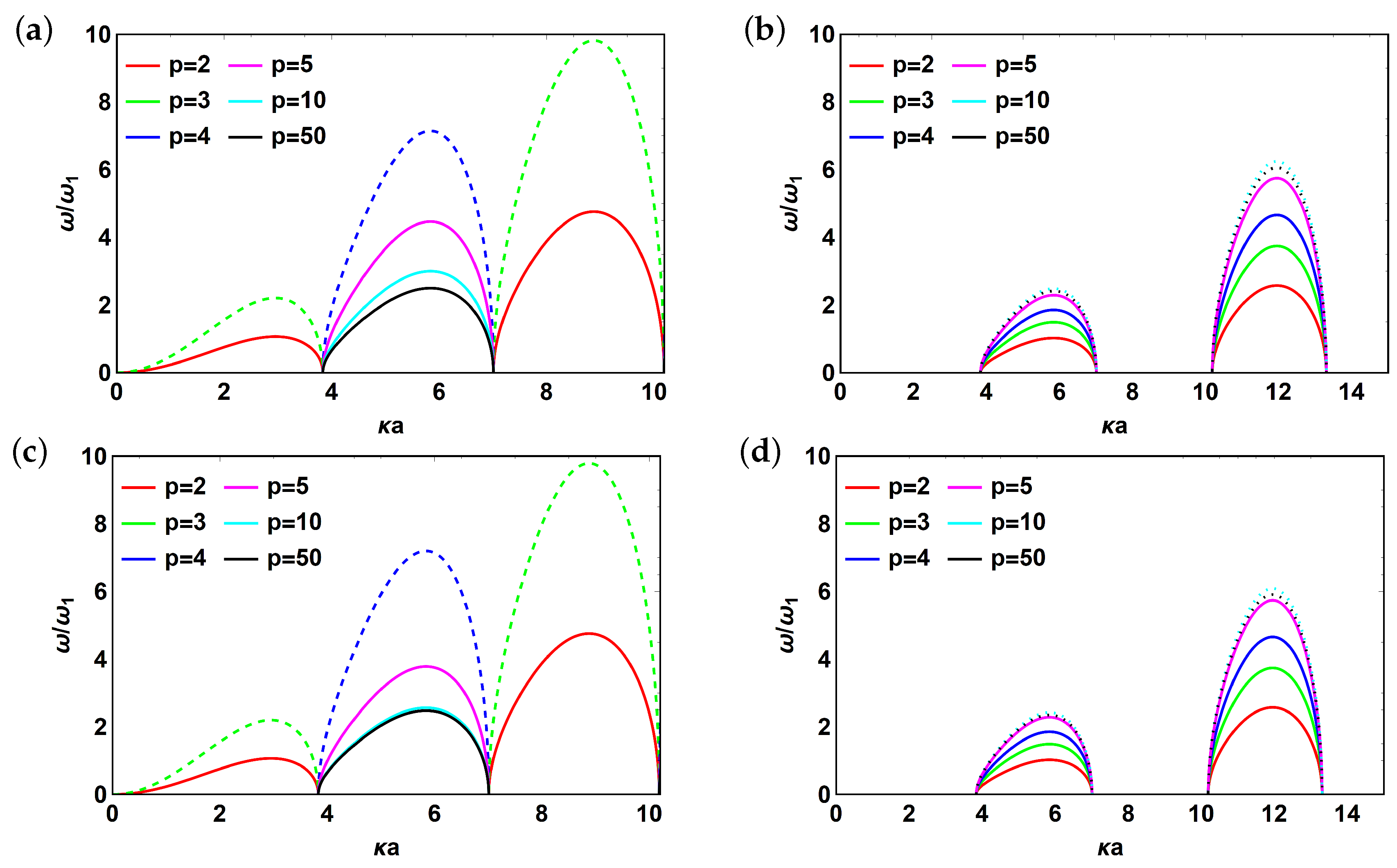
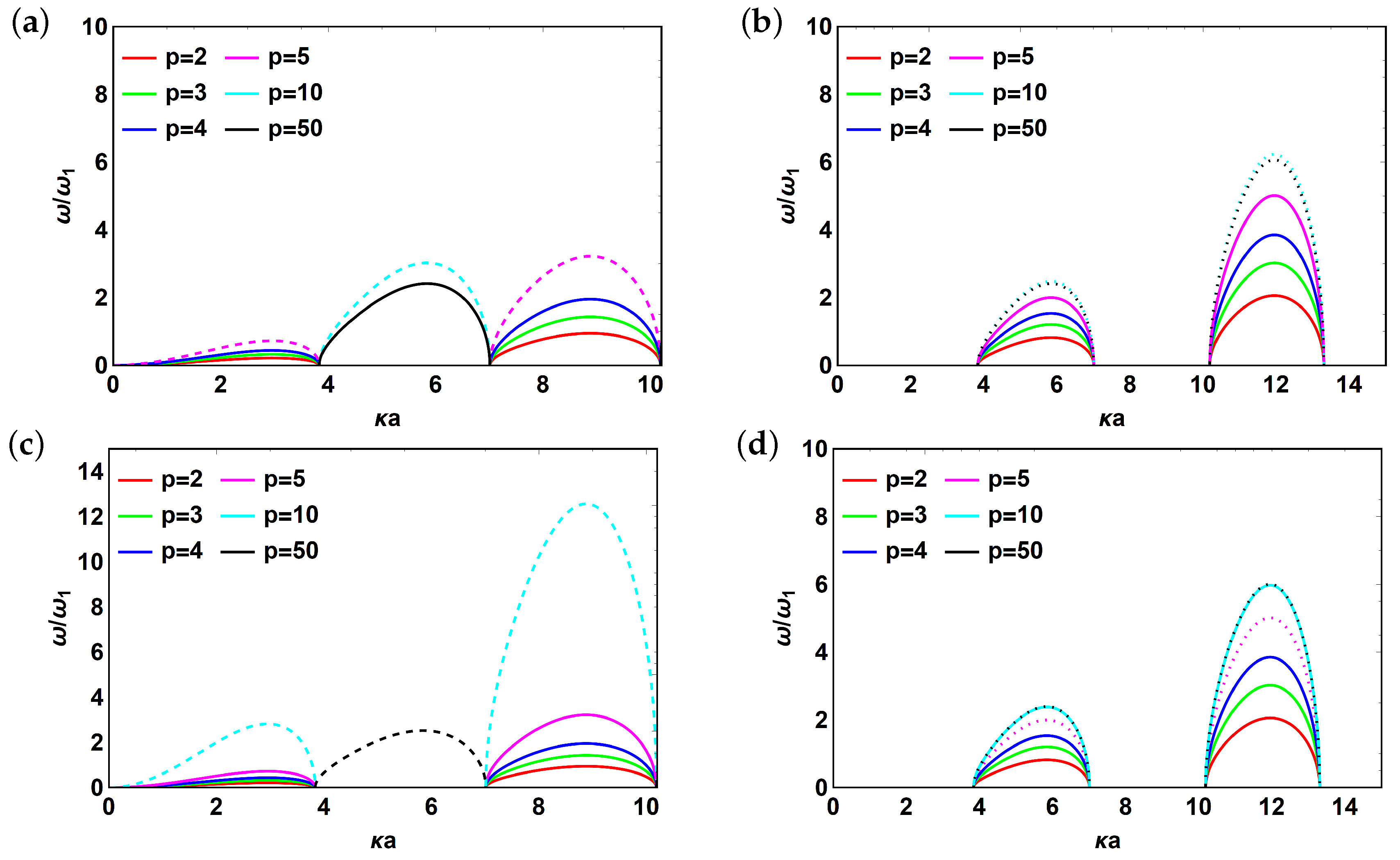
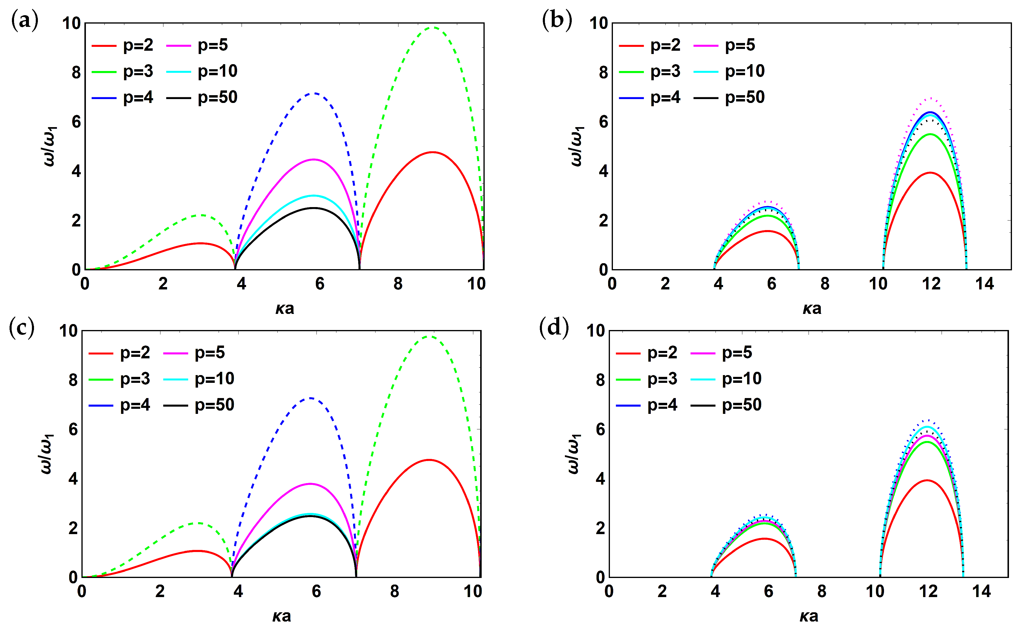
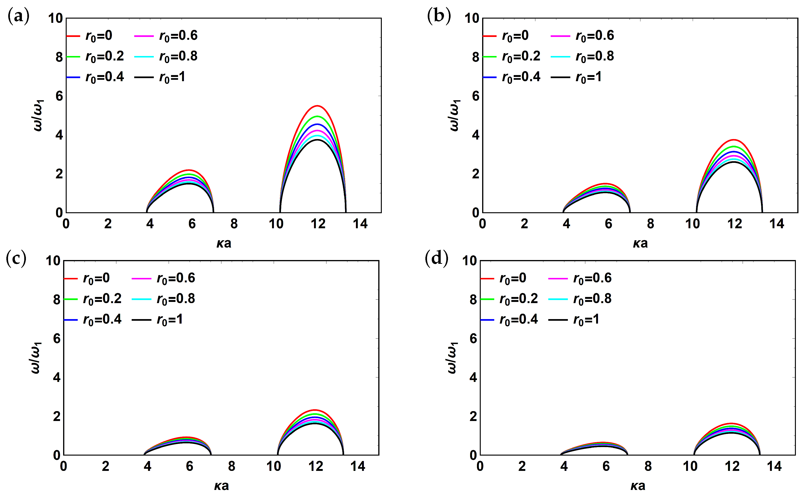
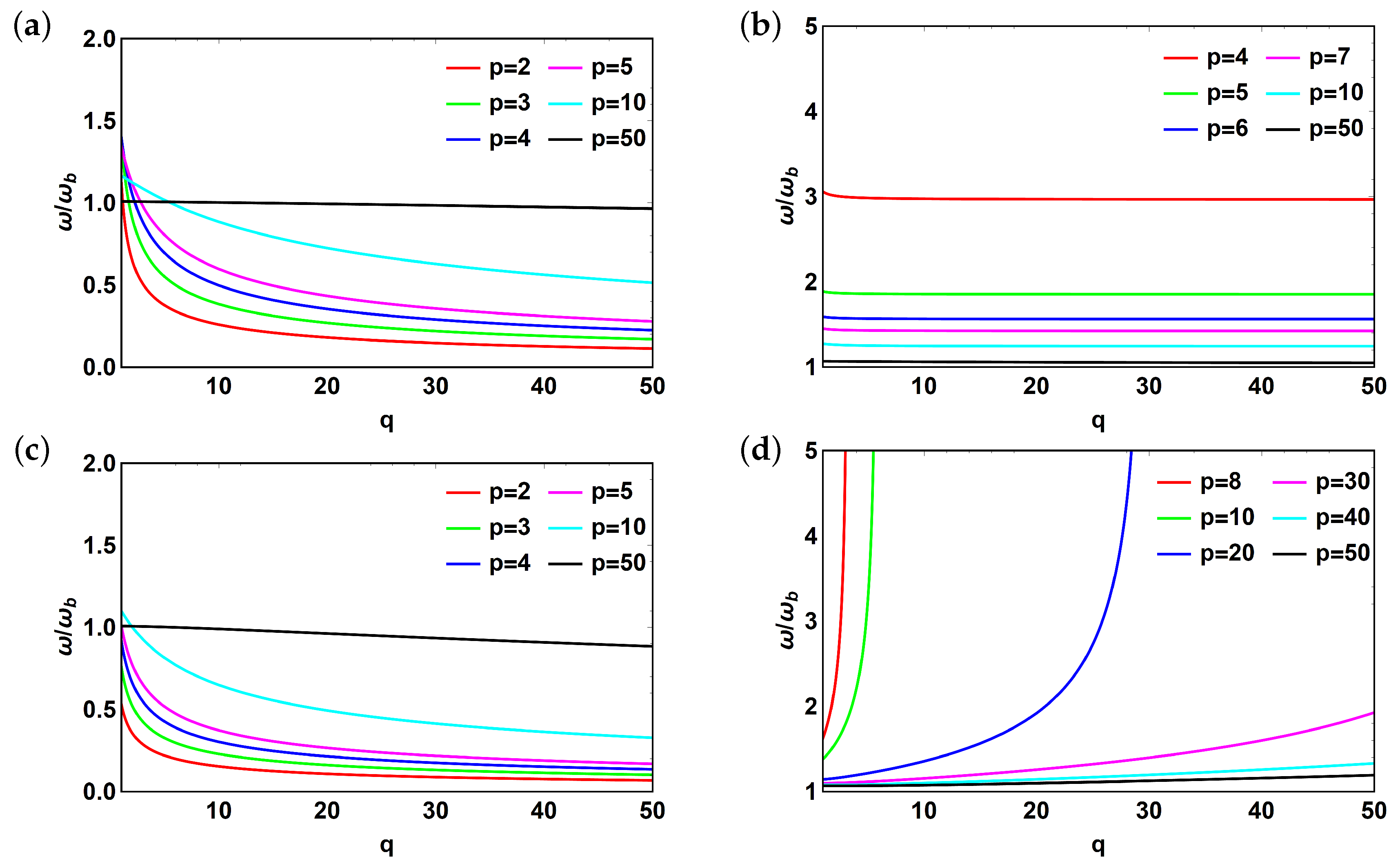
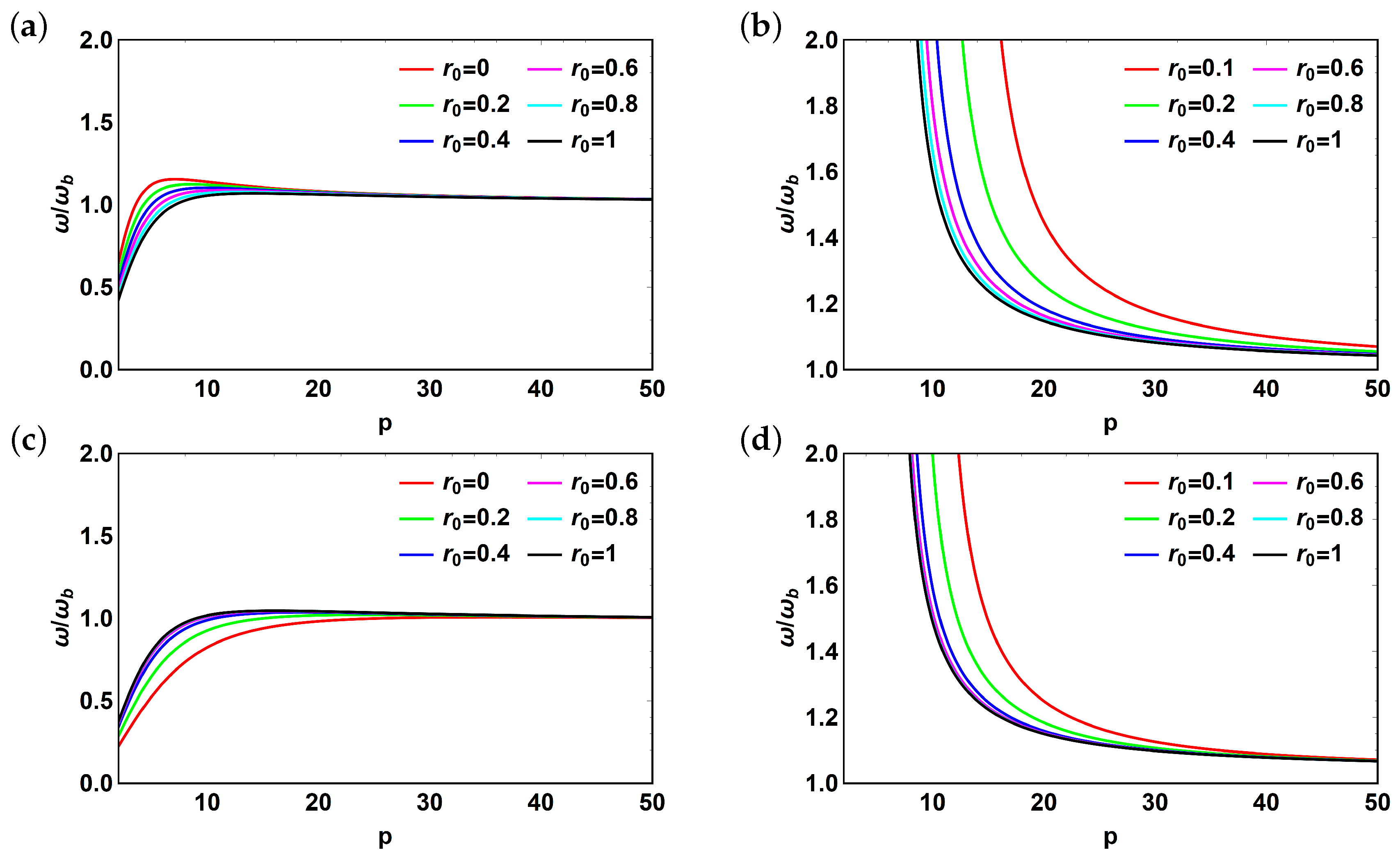
3.1. Metascreen Modes

To determine the resonant frequencies of the array, we should first know the resonant frequencies of the individual scatterer (trapped bubble). Instead of commonly used Minnaert frequency, we employ an approach proposed in [19] and developed in our previous work [18]. The modes of the interface vibrations read as [18]:

$${\omega }_b=\frac{\sqrt{{\kappa }_{mn}^3\sigma J_{-n}({\kappa }_{mn}a)({\rho }_1+{\rho }_2)-{\kappa }_{mn}^4{\eta }^2}}{{\rho }_1+{\rho }_2},$$

(16)

where $J_n({\kappa }_{mn}a)$ is the Bessel function of the first type of the order n, with ${\kappa }_{mn}$ being mode-dependent radial wave number. Here, we only account for the viscous damping. It is well known that for the clamped membrane multiple modes can be excited. However, we only pick the modes $(m,1)$ for our calculations. Once the resonant frequency of the individual scatterer was identified, we apply all of the analysis [13,14,20] to make the corrections to the resonant frequency of the system due to the strong coupling between the bubbles that allows shifting the resonant frequencies of the system.

The general approach to find resonant frequencies of the metamaterial includes two steps: (1) find $\Omega$ from extremal problem for energy transmission coefficient; and, (2) find $\omega$ from Equation (7). Let us first consider an array of bubbles positioned in the liquid bulk. Solving Equation (9), we arrive at:

$${\Omega }_{01}=0,$$

(17)

or in terms of resonant frequency:

$${\omega }_{01}=\frac{{\omega }_b}{\sqrt{1-A}},$$

(18)

where $A=\frac{2\sqrt{\pi }a}{d}$, a, and d stand for the bubble radius and distance between the centers of adjacent bubbles. Hereafter, we will use the notions of “negative” and “positive” branches of the solutions. These branches correspond to the values of ${\Omega }_i$ that has “−” and “+” in front of the “square root” terms. For instance, in Equation (19) ${\Delta }_0-\sqrt{{\delta }^2+{\Delta }_0^2}$ is a “negative” branch of the solution, whereas ${\Delta }_0+\sqrt{{\delta }^2+{\Delta }_0^2}$ is a “positive” one. The transmission dip given by Equation (18) is always present in the system, regardless of its complexity.

Next, let us assume the presence of the interface where the acoustic impedance changes abruptly from one side of the bubble array and bulk fluid from the other side. The interface can be formed by two media with different acoustic properties (e.g., water-air interface). Subsequently, solving Equation (18), we get:

$${\Omega }_{1,2}={\Delta }_0\pm \sqrt{{\delta }^2+{\Delta }_0^2},$$

(19)

where ${\Delta }_0=(B(1+h^2{k}^2)+2hk\delta )/2$. Here, $B=\frac{4\pi ah}{d^2}$ and h is the distance between the bubble’s center and adjacent interface. Subsequently, the resonant frequencies of the system read as:

$${\omega }_{01}=\frac{{\omega }_b}{\sqrt{1-A+{\Delta }_0+\sqrt{{\delta }^2+{\Delta }_0^2}}},{\omega }_{02}=\frac{{\omega }_b}{\sqrt{1-A+{\Delta }_0-\sqrt{{\delta }^2+{\Delta }_0^2}}}$$

(20)

Now, let us assume that $hk\ll 1$. Subsequently, Equation (19) becomes:

$${\Omega }_{1,2}=\frac{1}{2}\left(B\pm \sqrt{B^2+4{\delta }^2}\right)$$

(21)

and the resonant frequencies of the system read as:

$${\omega }_{01}=\frac{{\omega }_b}{\sqrt{1-A+B/2+\sqrt{{(B/2)}^2+{\delta }^2}}},{\omega }_{02}=\frac{{\omega }_b}{\sqrt{1-A+B/2-\sqrt{{(B/2)}^2+{\delta }^2}}}$$

(22)

Finally, if both $hk\ll 1$ and $\delta \ll 1$, the solution reduces to:

$${\Omega }_1=0,{\Omega }_2=B,$$

(23)

that results in two resonant frequencies of the system:

$${\omega }_{01}=\frac{{\omega }_b}{\sqrt{1-A}},{\omega }_{02}=\frac{{\omega }_b}{\sqrt{1-A+B}}$$

(24)

Similarly, if there are interfaces with abrupt acoustic impedance change from both sides of the bubble array, we obtain from Equation (13):

$${\Omega }_{1,2}={\Delta }_1\pm \sqrt{{\delta }^2+{\Delta }_1^2},$$

(25)

where ${\Delta }_1=(B+4hk\delta )/4$. Now, let us assume that $hk\ll 1$, Subsequently, Equation (25) becomes:

$${\Omega }_{1,2}=\frac{1}{4}\left(B\pm \sqrt{B^2+16{\delta }^2}\right)$$

(26)

and the resonant frequencies of the system read as:

$${\omega }_{01}=\frac{{\omega }_b}{\sqrt{1-A+B/4+\sqrt{{(B/4)}^2+{\delta }^2}}},{\omega }_{02}=\frac{{\omega }_b}{\sqrt{1-A+B/4-\sqrt{{(B/4)}^2+{\delta }^2}}}$$

(27)

Finally, if both $hk\ll 1$ and $\delta \ll 1$, the solution reduces to:

$${\Omega }_1=0,{\Omega }_2=B/2,$$

(28)

that results in two resonant frequencies of the system:

$${\omega }_{01}=\frac{{\omega }_b}{\sqrt{1-A}},{\omega }_{02}=\frac{{\omega }_b}{\sqrt{1-A+B/2}}$$

(29)

Solutions given by Equations (24) and (29) are identical to Equation (2) from [14], where the dissipation factor was neglected.

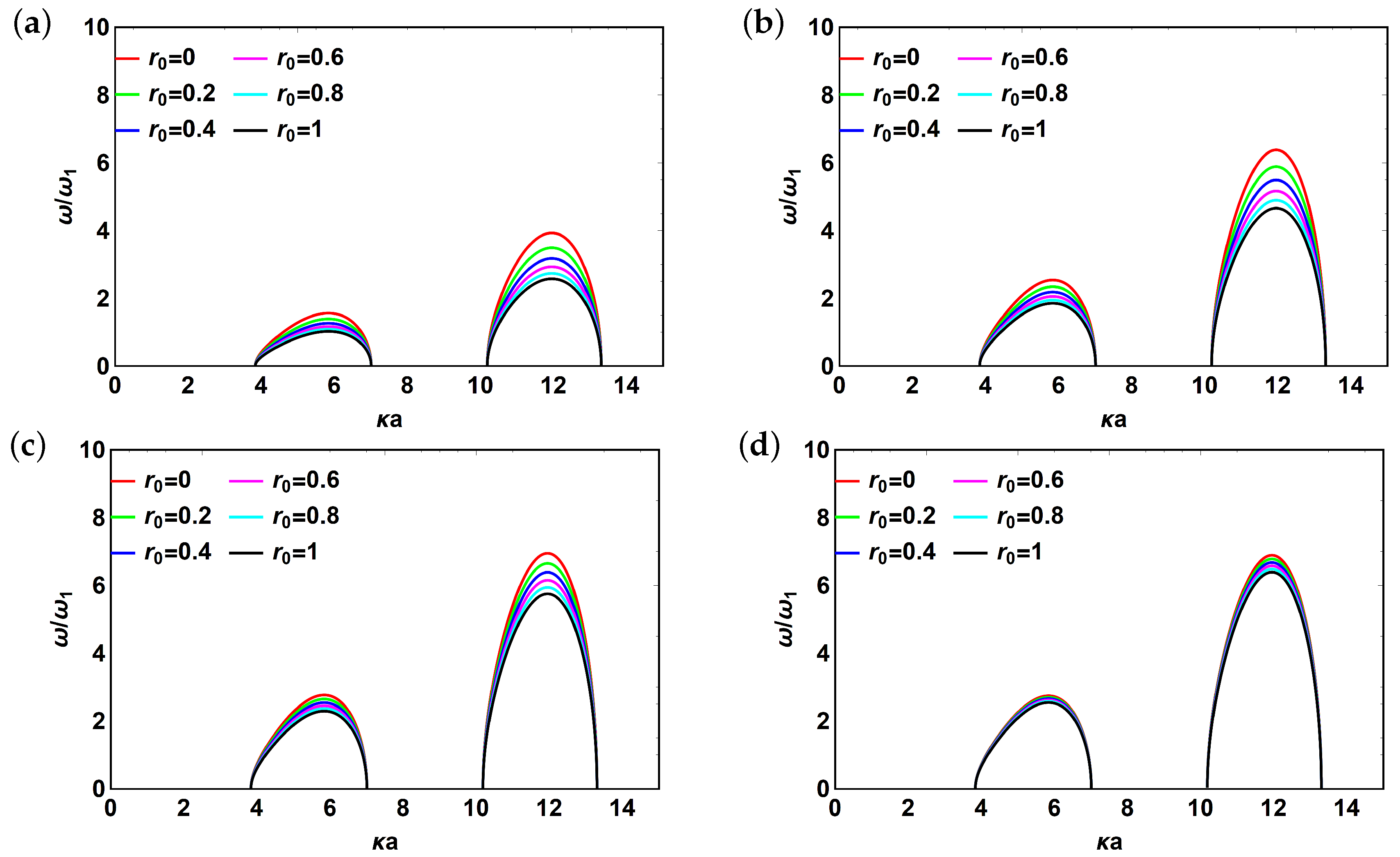
3.2. Reflector Effect

We will now apply the technique developed above to solve the same problems in the case of presence of reflector in a vicinity of metatamaterial. Let us consider a case of a single interface first. Assuming that $hk\ll 1$, ${\Omega }_i$ read as:

$${\Omega }_{1,2}={\Gamma }_3\pm \sqrt{{\Delta }_3^2+{\delta }^2},$$

(30)

where ${\Gamma }_3$ and ${\Delta }_3$ are given by:

$${\Gamma }_3=\frac{B(-1+r_0^2)}{2r_0},{\Delta }_3=\frac{B{(1+r_0)}^2}{2r_0}$$

(31)

Afterwards, the resonant frequencies of the system read as:

$${\omega }_{01}=\frac{{\omega }_b}{\sqrt{1-A+{\Gamma }_3+\sqrt{{\Delta }_3^2+{\delta }^2}}},{\omega }_{02}=\frac{{\omega }_b}{\sqrt{1-A+{\Gamma }_3-\sqrt{{\Delta }_3^2+{\delta }^2}}}$$

(32)

If both $hk\ll 1$ and $\delta \ll 1$ the solution reduces to:

$${\Omega }_{1,2}={\Gamma }_3\pm {\Delta }_3$$

(33)

Subsequently, the resonant frequencies of the system are:

$${\omega }_{01}=\frac{{\omega }_b}{\sqrt{1-A+{\Gamma }_3+{\Delta }_3}},{\omega }_{02}=\frac{{\omega }_b}{\sqrt{1-A+{\Gamma }_3-{\Delta }_3}}$$

(34)

or in more explicit form:

$${\omega }_{01}=\frac{{\omega }_b}{\sqrt{1-A+B(1+r_0)}},{\omega }_{02}=\frac{{\omega }_b}{\sqrt{1-A-B\left(1+\frac{1}{r_0}\right)}}$$

(35)

Analogous to this, in case of two interfaces near the bubble metascreen for $hk\ll 1$, we obtain:

$${\Omega }_{1,2}={\Gamma }_4\pm \sqrt{{\Delta }_4^2+{\delta }^2},$$

(36)

where ${\Gamma }_4$ and ${\Delta }_4$ are given by:

$${\Gamma }_4=\frac{B(-1+r_0^2)}{4r_0},{\Delta }_4=\frac{B{(1+r_0)}^2}{4r_0}$$

(37)

Subsequently, the resonant frequencies of the system read as:

$${\omega }_{01}=\frac{{\omega }_b}{\sqrt{1-A+{\Gamma }_4+\sqrt{{\Delta }_4^2+{\delta }^2}}},{\omega }_{02}=\frac{{\omega }_b}{\sqrt{1-A+{\Gamma }_4-\sqrt{{\Delta }_4^2+{\delta }^2}}}$$

(38)

If both $hk\ll 1$ and $\delta \ll 1$ the solution reduces to:

$${\Omega }_{1,2}={\Gamma }_4\pm {\Delta }_4$$

(39)

Afterwards, the resonant frequencies of the system are:

$${\omega }_{01}=\frac{{\omega }_b}{\sqrt{1-A+{\Gamma }_4+{\Delta }_4}},{\omega }_{02}=\frac{{\omega }_b}{\sqrt{1-A+{\Gamma }_4-{\Delta }_4}}$$

(40)

or in more explicit form:

$${\omega }_{01}=\frac{{\omega }_b}{\sqrt{1-A+\frac{B}{2}(1+r_0)}},{\omega }_{02}=\frac{{\omega }_b}{\sqrt{1-A-\frac{B}{2}\left(1+\frac{1}{r_0}\right)}}$$

(41)

3.3. Numerical Validation

Now, let us examine dispersion relations for all of the frequencies obtained above. Introduce non-dimensional quantities $p=d/a$ and $q=h/a$ for convenience and consider the behavior of modes $(m,1)$ normalized by mode $(0,1)$. The case of 1 interface without reflector is shown in Figure 2. Figure 2a represents the case without interface and without reflector (given by Equation (18)) and it is provided for reference. Figure 2b,d correspond to ${\omega }_{01}$ from Equation (24) and ${\omega }_{02}$ from Equation (22). The plots look pretty similar due to relatively low value of dissipation factor ($\delta =0.05$) and demonstrate the presence of bandgaps while the values of the resonant peaks increase with increasing p until hardly recognizable maximum (compare $p=10$ and $p=50$) and then reaches saturation. Large values of p correspond to the case of independent scatterers. Finally, Figure 2c corresponds to ${\omega }_{02}$ from Equation (22). The behavior of dispersion curve changes dramatically as p increases from $p=3$ to $p=4$. More specifically switching between the modes happens. Hereafter, under “switching” between modes we understand changing dispersion curve position along horizontal axis that corresponds to a different value of $\kappa a$. Moreover, the value of the resonant peak increases before mode switching and starts to decrease after it.

Figure 3 shows the case of 1 interface with reflector featuring amplitude reflection coefficient $r_0=0.5$. Figure 3a,c correspond to ${\omega }_{02}$ from Equations (32) and (35), respectively. The difference between them is that Figure 3a neglects the dissipation, while Figure 3c accounts for it. The switching between modes is observed in both cases, while it happens for higher values of p if dissipation is considered. For ${\omega }_{01}$ from Equations (32) and (35) (Figure 3b,d, respectively) no switching is observed and the solutions look pretty much similar. If compared with Figure 2b,d, no maximum value of the peak is visible, while only increasing with p until saturation in case of independent scatterers. It can also be seen that in presence of reflector peak values reduce significantly.

Figure 4 and Figure 5 provide the similar plots for two interfaces. For “negative” branch, there is a usual switching between modes that, however, also differs in case of absence (Figure 4a,c) and presence of reflector (Figure 5a,c) with the later exhibiting lower values of the resonant peak. As for “positive” branch of the solution, there is, again, no switching between the mode is observed while the peak values visibly increase, reach maximum, and decrease down to saturation with increasing p.

Next, we consider the effect of reflector explicitly, by fixing one of the geometry parameters $p,q$ and varying another one along with the amplitude reflection coefficient, $r_0$. Let us first fix $q=1$ (the smallest possible value that represents the case of a reflector positioned just next to the bubble array) and vary $p=2\dots 10$ and $r_0=0\dots 1$.

Figure 6 shows the corresponding dispersion relation. As can be seen from it, no switching between modes is observed while the value of the resonant peak decreases (from red to black plot) monotonically with increasing $r_0$. This trend remains the same with p increasing. At the same time, the effect of variation in amplitude reflection coefficient becomes smaller as p increases.

Alternatively, we fix $p=3$ and vary $q=1\dots 10$ along with $r_0=0\dots 1$, as shown in Figure 7. In this case, the maximum values of the peak decrease monotonically with both $r_0$ and q increasing and several bandgaps are present, as previously.

Now, let us examine the behavior of the system resonant frequency normalized by that of a single bubble with respect to geometry parameters p and q. In Figure 8, the dependence of normalized system frequency from p for case of 2 interfaces with and without reflector is shown. For all values of q and all solution branches normalized frequency tends to 1 for large values of p that corresponds to the case of independent scatterers. For “positive” branch of the solution (Figure 8a,c) the presence of the reflector flattens the resonant peak observed for small values of p (strongly coupled bubbles). The behavior of normalized frequency also changes from resonant to monotonically increasing until saturation with increasing q. A completely different behavior is observed for “negative” branch of the solution (Figure 8b,d). In particular, the system experiences abrupt monotonic decay of normalized frequency starting from a certain value of p that is almost independent from q if the reflector is absent. The situation changes when the reflector is added. In this case, the starting point of abrupt decay shifts to higher values of p with increasing q.

Figure 9 shows the dependence of normalized system frequency as a function of q. Similar to above, we consider the case with two interfaces with and without reflector. For “positive” branch of the solution (Figure 9a) the presence of reflector (Figure 9c) does not effect the behavior of the system. The normalized frequency decreases monotonically with increasing q and tends to 1 with increasing p. However, the situation changes for “negative” branch of the solution. If the reflector is absent (Figure 9b) the normalized frequency does not change with q and decreases with increasing p. If the reflector is present (Figure 9d), the normalized frequency increases abruptly with increasing q. However, the trend becomes more moderate with increasing p until it becomes independent of q for large values of p.

Finally, consider the case of varying reflection coefficient, $r_0$. It is shown in Figure 10. Here, we fix $q=1$ (lowest possible value) and examine the behavior of normalized frequency of the system with p. In Figure 10a,c the “positive” branch of the solution is presented without (Figure 10a) and with dissipation (Figure 10c). The trend is overall repeatable with normalized frequency reaching saturation for large p. The dramatic difference is that for small dissipation the rate of reaching saturation decreases with increasing $r_0$ whereas it increases with increasing $r_0$ when dissipation is taken into account. For “negative” branch of the solution (Figure 10b,d) the trend is almost the same: abrupt decrease of normalized frequency with increasing p. However, the starting point of abrupt decay moves to lower values of p with increasing $r_0$, opposite to the trend observed in Figure 8d.

4. Conclusions

We have developed a theoretical model to predict the resonant behavior of bubble-based metamaterials. The dispersion relations for the bubble array in bulk and in a vicinity of one and two interfaces of acoustic impedance abrupt change were derived. Different degrees of accuracy of the solution were investigated, accounting for dissipation and neglecting it. Multiple bandgaps are predicted for all the solutions. Moreover, for the solutions in bulk and without interface as well as for “negative” branches of the solution (1 and 2 interfaces, with and without reflector) the switching between bandgaps is predicted. For “positive” branches of the solutions bandgaps are predicted to be stable. The system behavior can be adjusted with both geometrical parameters and reflector properties. In particular, an increase of the distance between bubble centers (decoupling) results in either non-monotonous behavior of system resonant frequency (“negative” branch) or its monotonic increase up to saturation/increase up to peak followed by decay to constant value (“positive” branch). In contrast, an increase in amplitude reflection coefficient results in a monotonic decrease of the system resonant frequency. These results clearly demonstrate that various regimes of metamaterial operation can be achieved via fine tuning of resonant frequency of the system, adjusting its geometry and reflector properties.

The following is worth noting. While here we report theoretical developments, the general approach employed to describe resonant behavior of bubble array structures has been experimentally verified in previous studies [13,22].

References

1. Veselago, V.G. The electrodynamics of substances with simultaneously negative values of and µ. Sov. Phys. Usp. 1968, 10, 509. [Google Scholar] [CrossRef]
2. Commander, K.W.; Prosperetti, A. Linear pressure waves in bubbly liquids: Comparison between theory and experiments. J. Acoust. Soc. Am. 1989, 85, 732–746. [Google Scholar] [CrossRef]
3. Pendry, J.B. Negative refraction makes a perfect lens. Phys. Rev. Lett. 2000, 85, 3966. [Google Scholar] [CrossRef]
4. Cummer, S.A.; Christensen, J.; Alù, A. Controlling sound with acoustic metamaterials. Nat. Rev. Mater. 2016, 1, 1–13. [Google Scholar] [CrossRef] [Green Version]
5. Iannace, G.; Berardi, U.; Ciaburro, G.; Trematerra, A. Sound Attenuation of an Acoustic Barrier Made with Metamaterials. 2019. Available online: https://jcaa.caa-aca.ca/index.php/jcaa/article/view/3308 (accessed on 18 August 2020).
6. Milton, G.W.; Willis, J.R. On modifications of Newton’s second law and linear continuum elastodynamics. Proc. R. Soc. R. Soc. 2007, 463, 855–880. [Google Scholar] [CrossRef]
7. Yao, S.; Zhou, X.; Hu, G. Experimental study on negative effective mass in a 1D mass–spring system. New J. Phys. 2008, 10, 043020. [Google Scholar] [CrossRef]
8. Huang, H.; Sun, C.; Huang, G. On the negative effective mass density in acoustic metamaterials. Int. J. Eng. Sci. 2009, 47, 610–617. [Google Scholar] [CrossRef]
9. Huang, G.; Sun, C. Band gaps in a multiresonator acoustic metamaterial. J. Vib. Acoust. 2010, 132, 031003. [Google Scholar] [CrossRef] [Green Version]
10. Tan, K.T.; Huang, H.; Sun, C. Optimizing the band gap of effective mass negativity in acoustic metamaterials. Appl. Phys. Lett. 2012, 101, 241902. [Google Scholar] [CrossRef]
11. Manimala, J.M.; Sun, C. Microstructural design studies for locally dissipative acoustic metamaterials. J. Appl. Phys. 2014, 115, 023518. [Google Scholar] [CrossRef]
12. Chen, Y.; Barnhart, M.; Chen, J.; Hu, G.; Sun, C.; Huang, G. Dissipative elastic metamaterials for broadband wave mitigation at subwavelength scale. Compos. Struct. 2016, 136, 358–371. [Google Scholar] [CrossRef]
13. Leroy, V.; Strybulevych, A.; Scanlon, M.; Page, J. Transmission of ultrasound through a single layer of bubbles. Eur. Phys. J. E 2009, 29, 123–130. [Google Scholar] [CrossRef]
14. Bretagne, A.; Tourin, A.; Leroy, V. Enhanced and reduced transmission of acoustic waves with bubble meta-screens. Appl. Phys. Lett. 2011, 99, 221906. [Google Scholar] [CrossRef]
15. Lanoy, M.; Guillermic, R.M.; Strybulevych, A.; Page, J.H. Broadband coherent perfect absorption of acoustic waves with bubble metascreens. Appl. Phys. Lett. 2018, 113, 171907. [Google Scholar] [CrossRef] [Green Version]
16. Cai, Z.; Zhao, S.; Huang, Z.; Li, Z.; Su, M.; Zhang, Z.; Zhao, Z.; Hu, X.; Wang, Y.S.; Song, Y. Bubble Architectures for Locally Resonant Acoustic Metamaterials. Adv. Funct. Mater. 2019, 29, 1906984. [Google Scholar] [CrossRef]
17. Leroy, V.; Bretagne, A.; Lanoy, M.; Tourin, A. Band gaps in bubble phononic crystals. AIP Adv. 2016, 6, 121604. [Google Scholar] [CrossRef] [Green Version]
18. Gritsenko, D.; Lin, Y.; Hovorka, V.; Zhang, Z.; Ahmadianyazdi, A.; Xu, J. Vibrational modes prediction for water-air bubbles trapped in circular microcavities. Phys. Fluids 2018, 30, 082001. [Google Scholar] [CrossRef] [Green Version]
19. Chindam, C.; Nama, N.; Ian Lapsley, M.; Costanzo, F.; Jun Huang, T. Theory and experiment on resonant frequencies of liquid-air interfaces trapped in microfluidic devices. J. Appl. Phys. 2013, 114, 194503. [Google Scholar] [CrossRef] [Green Version]
20. Leroy, V.; Strybulevych, A.; Lanoy, M.; Lemoult, F.; Tourin, A.; Page, J.H. Superabsorption of acoustic waves with bubble metascreens. Phys. Rev. B 2015, 91, 020301. [Google Scholar] [CrossRef] [Green Version]
21. Gupta, A. A review on sonic crystal, its applications and numerical analysis techniques. Acoust. Phys. 2014, 60, 223–234. [Google Scholar] [CrossRef]
22. Leroy, V.; Bretagne, A.; Fink, M.; Willaime, H.; Tabeling, P.; Tourin, A. Design and characterization of bubble phononic crystals. Appl. Phys. Lett. 2009, 95, 171904. [Google Scholar] [CrossRef] [Green Version]
Figure 1. Domain definition for (a) single bubble; (b) bubble array; (c) bubble array with reflector. Numbers 1 and 2 in (a) correspond to subscripts in Equation (3).
Applsci 10 05720 g001
Figure 2. Dispersion relation for metascreen (a) w/o interface and w/o reflector; (b) w/1 interface and w/o reflector, k h 1 , δ 1 ; (c) w/1 interface and w/o reflector, k h 1 , “negative” branch; (d) w/1 interface and w/o reflector, k h 1 , “positive” branch. For all plots n = 1 , q = 2 . Dashed lines in (a,c) are used to demonstrate switching between modes; dotted lines in (b,d) demonstrate the largest resonant peak for various configurations of metamaterial and compare it with the case of independent scatterers (black curve).
Applsci 10 05720 g002
Figure 3. Dispersion relation for metascreen (a) w/1 interface and w/reflector ( r 0 = 0.5 ), k h 1 , δ 1 , “negative” branch; (b) w/1 interface and w/reflector ( r 0 = 0.5 ), k h 1 , δ 1 , “positive” branch; (c) w/1 interface and w/reflector ( r 0 = 0.5 ), k h 1 , “negative” branch; (d) w/1 interface and w/reflector ( r 0 = 0.5 ), k h 1 , “positive” branch. For all plots n = 1 , q = 2 . Dashed lines in (a,c) are used to demonstrate switching between modes; dotted lines in (b,d) demonstrate the largest resonant peak for various configurations of metamaterial and compare it with the case of independent scatterers (black curve).
Applsci 10 05720 g003
Figure 4. Dispersion relation for metascreen (a) w/o interface and w/o reflector; (b) w/2 interfaces and w/o reflector, k h 1 , δ 1 ; (c) w/2 interfaces and w/o reflector, k h 1 , “negative” branch; (d) w/2 interfaces and w/o reflector, k h 1 , “positive” branch. For all plots n = 1 , q = 2 . Dashed lines in (a,c) are used to demonstrate switching between modes; dotted lines in (b,d) demonstrate the largest resonant peak for various configurations of metamaterial and compare it with the case of independent scatterers (black curve).
Applsci 10 05720 g004
Figure 5. Dispersion relation for metascreen (a) w/2 interfaces and w/reflector ( r 0 = 0.5 ), k h 1 , δ 1 , “negative” branch; (b) w/2 interfaces and w/reflector ( r 0 = 0.5 ), k h 1 , δ 1 , “positive” branch; (c) w/2 interfaces and w/reflector ( r 0 = 0.5 ), k h 1 , “negative” branch; (d) w/2 interfaces and w/reflector ( r 0 = 0.5 ), k h 1 , “positive” branch. For all plots n = 1 , q = 2 . Dashed lines in (a,c) are used to demonstrate switching between modes; dotted lines in (b,d) demonstrate the largest resonant peak for various configurations of metamaterial and compare it with the case of independent scatterers (black curve).
Applsci 10 05720 g005
Figure 6. Dispersion relation for metascreen w/1 interface and w/reflector (a) q = 1 , p = 2 ; (b) q = 1 , p = 4 ; (c) q = 1 , p = 6 ; (d) q = 1 , p = 10 . For all plots n = 1 , r 0 = 0.5 , k h 1 , δ 1 . “Positive” branch only is shown.
Applsci 10 05720 g006
Figure 7. Dispersion relation for metascreen w/1 interface and w/reflector (a) q = 1 , p = 3 ; (b) q = 2 , p = 3 ; (c) q = 5 , p = 3 ; (d) q = 10 , p = 3 . For all plots n = 1 , r 0 = 0.5 , k h 1 , δ 1 . “Positive” branch only is shown.
Applsci 10 05720 g007
Figure 8. Normalized frequency as a function of p (distance between bubble centers) for metascreen (a) w/2 interfaces and w/o reflector, “positive” branch, k h 1 ; (b) w/2 interfaces and w/o reflector, “negative” branch, k h 1 ; (c) w/2 interfaces and w/reflector ( r 0 = 0.5 ), “positive” branch, k h 1 ; (d) w/2 interfaces and w/reflector ( r 0 = 0.5 ), “negative” branch, k h 1 .
Applsci 10 05720 g008
Figure 9. Normalized frequency as a function of q (distance between bubble center and interface) for metascreen (a) w/2 interfaces and w/o reflector, “positive” branch, k h 1 ; (b) w/2 interfaces and w/o reflector, “negative” branch, k h 1 ; (c) w/2 interfaces and w/reflector ( r 0 = 0.5 ), “positive” branch, k h 1 ; (d) w/2 interfaces and w/reflector ( r 0 = 0.5 ), “negative” branch, k h 1 .
Applsci 10 05720 g009
Figure 10. Normalized frequency as a function of p (distance between bubble centers) for metascreen (a) w/1 interface and w/reflector, “positive” branch, k h 1 , δ 1 ; (b) w/1 interface and w/reflector, “negative” branch, k h 1 , δ 1 ; (c) w/1 interface and w/reflector, “positive” branch, k h 1 ; (d) w/1 interface and w/reflector, “negative” branch, k h 1 . For all plots q = 1 .
Applsci 10 05720 g010