Experimental and Numerical Investigation of the Internal Temperature of an Oil-Immersed Power Transformer with DOFS

Abstract

To accurately detect and monitor the internal temperature of an operating power transformer, the distributed optical fiber sensor (DOFS) was creatively applied inside an oil-immersed 35 kV transformer through high integration with the winding wire. On the former basis, the power transformer prototype with a completely global internal temperature sensing capability was successfully developed and it was also qualified for power grid operation through the ex-factory type tests. The internal spatially continuous temperature distribution of the operating transformer was then revealed through a heat-run test and the numerical simulation was also applied for further analysis. Hotspots of windings were continuously located and monitored (emerging at about 89%/90% height of low/high voltage winding), which were furtherly compared with the IEC calculation results. This new nondestructive internal sensing method shows a broad application prospect in the electrical equipment field. Also, the revelation of transformer internal distributed temperature can offer a solid reference for both researchers and field operation staff.

1. Introduction

Transformer is the core equipment of power systems, and its safe operation is of great significance to the stability of the power supply. The failure of a large power transformer often leads to a blackout in an entire area, causing huge economic losses. As such real-time dynamic monitoring of the online transformer status has aroused wide interest [1,2,3].

The internal temperature of a transformer, especially the winding hotspot, has a direct influence on the insulation performance and its service life. Overheating during operation will decrease the life expectancy of the insulated materials and thus threaten the safety of the local grid, while running at a lower temperature means less load and the sacrifice of economic benefits [4]. Hence, the optimal balance between safety and economy requires actual data-based criterion to grasp. Moreover, the dynamic capacity-increasing and energy-saving control of the transformers are both empirical models, still lacking quantitative, reliable support [5]. It is therefore necessary to obtain the real time temperature distribution inside the transformer.

Currently, the traditional transformer temperature monitoring methods can be primarily divided into four types: empirical formula method [6,7], numerical simulation, infrared measurements [8,9] and contact measurements (including thermocouples, fiber Bragg grating (FBG) and fluorescence optical fiber, etc.) [10,11].

Among them, the empirical formula method has gradually become mature after many amendments since it was first proposed in 1911 and has been widely applied in actual operations [12]. In IEC 60076 standard, different coefficients are suggested for transformers with different heat dissipation modes, which can be directly used for the temperature calculation of transformer hotspots under different load conditions and operating conditions [13]. This method can reflect the relationship between the hotspot temperature and the transformer operating state. It is simple and thus has a wide range of applications [6]. However, it has been proved that in some cases, the calculation result holds a large error compared with the actual measurements [14]. Meanwhile, it is also difficult to keep pace with the instantaneous load changes, which inevitably leads to the lack of real-time response [15]. Therefore, the empirical formula based detecting method is more suitable for a rough but fast calculation.

However, the method above only focuses on the hotspot temperature, lacking the thermal information of the entire internal area. The numerical simulation, which establishes the partial differential equations for the internal convective heat exchange process according to the fluid mechanics, could solve this problem theoretically through a global computing by relevant algorithms [16]. J. Mufuta and El Wakiln were the first to make great progress in this area through a 2D thermodynamic modelling of an oil-immersed transformer [17,18]. Then, J. Smolka further obtained a more detailed 3D temperature distribution by combining genetic algorithms with the multi-physics coupling [19]. In order to reduce the modelling complexity, J. Gastelurrutia furtherly simplified the transformer heat source and boundary conditions, and hereby proposed an equivalent calculation model [20]. However, limited by the inevitable simplifications and the convergence of algorithms, the simulation result usually has deviations in reflecting the real state of a transformer, and in most cases, it only serves as a theoretical reference [21].

Besides the aforesaid calculation methods, direct detection usually stands out for its simple and intuitive properties. The remote non-contact measurement with infrared camera is convenient for people to operate, but it can be easily affected by the ambient temperature, electromagnetic signals or the shooting position, bringing inevitable measurement errors [8]. Moreover, this camera-based method is also unable to measure the internal temperature distribution of a transformer in real time. Thus, the infrared detection could only provide an external overall thermal situation.

In comparison, the contact measurement is a method to detect the temperature of a certain position inside the transformer by thermocouples, fluorescent fiber, fiber gratings, etc. It is simple and effective, but the location of the sensor has a strong empirical dependence and it still cannot realize the whole area temperature sensing, leaving a large monitoring blind area [11]. The remarkable achievement was a measurement performed in 2012 by Kweon on a 154 kV transformer during the temperature-rise test. The fluorescent fiber sensors were placed in advance on the windings for a local temperature measurement [22]. This was followed by Arabul, who had arranged large quantities of fluorescent fiber sensors in the oil passages between each adjacent winding wire for the detection of overheated regions in a 1.5 MVA transformer [23]. However, affected by the complicated circumstances inside transformer, the different positions chosen for the sensors may lead to different results. There are also leaving numerous sensor probes and complex internal leads. Some new horizons are thereby required to minimize the monitoring blind zones.

The distributed optical fiber sensing technology, developing rapidly in recent years, has gradually applied in some super projects like geo-environmental monitoring, bridge and tunnel monitoring, petroleum and gas lines monitoring, power lines monitoring, and so forth, due to its spatiotemporally continuous monitoring and excellent real-time performance. Among these, the ROTDR (Raman Optical Time Domain Reflection) technology has been successfully applied by NASA (National Aeronautics and Space Administration) and ANDRA (French National Radioactive Waste Management Agency) in the harshest environments such as a space shuttle [24] and an underground nuclear waste repository [25]. Yahei, from Japan, has further obtained a 0.01 °C temperature resolution through coherent OTDR (Optical Time Domain Reflection) technology [26]. Lu has applied the DOFS to a laboratory energized transformer core based on Rayleigh scattering, but its limited detecting range is hard to monitor the field power transformer [27]. In commercial products, the Sensornet ltd (Hertfordshire, British) has reached a resolution of 0.02 °C per meter along the sensing fiber for 45 km in each direction, and can withstand up to 700 °C in a corrosive situation [28].

Therefore, it exhibits great potential for DOFS (Distributed Optical Fiber Sensor) application in the electrical apparatus field. In this contribution, according to the actual structures of an oil-immersed 35 kV power transformer, different laying schemes were designed for the DOFS. Verified by the corresponding tests, the transformer prototype with built-in distributed sensing fibers was successfully developed and was up to standard for power grid operation through the ex-factory type tests. Moreover, the internal real-time online temperature of an operating power transformer was also revealed in a distributed manner. The hotspots were accurately located and continuously monitored. Assisted by numerical simulations, the actual detected data were also compared with the IEC traditional calculation results. These first-hand data may provide a solid reference for the delicate management of power transformers.

2. Sensing Principle

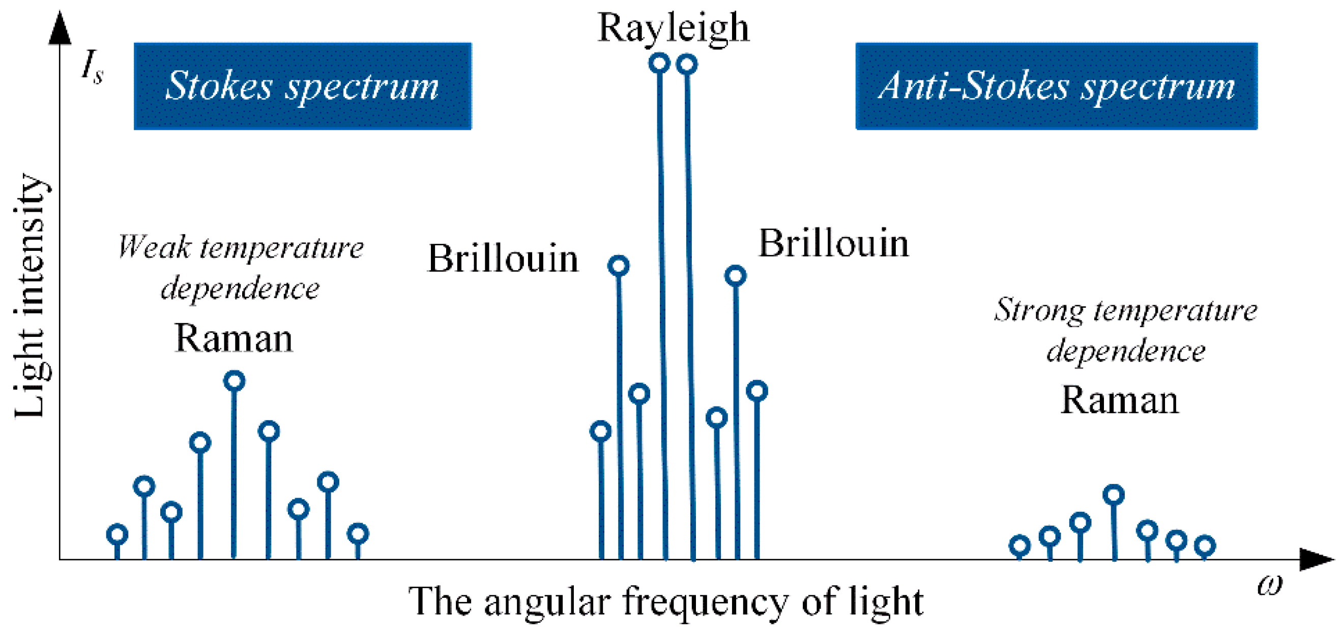
When light transmits in an optical fiber, the light waves will be scattered to different degrees under the influence of medium molecules, resulting in a scattering spectrum with different frequencies [28]. Thus, the elastic scattering (Rayleigh scattering) and inelastic scattering (Brillouin scattering and Raman scattering) can be identified according to their frequency (Figure 1). While Raman scattering, including two different frequency parts, has been discovered to have a strong temperature sensitivity among these scattered lights, especially in its high frequency region.

When light propagates through the fiber, the luminous flux of Stokes Raman scattering generated by each light pulse [29] is presented in Equation (1):

$${\Phi }_S=K_S\cdot S\cdot v_S^4\cdot {\varphi }_e\cdot R_S(T)\cdot \exp [-({\alpha }_0+{\alpha }_S)\cdot L]$$

(1)

The luminous flux of anti-Stokes Raman scattering can be expressed as Equation (2):

$${\Phi }_{AS}=K_{AS}\cdot S\cdot v_{AS}^4\cdot {\varphi }_e\cdot R_{AS}(T)\cdot \exp [-({\alpha }_0+{\alpha }_{AS})\cdot L]$$

(2)

where K_S and K_AS are the cross-section coefficients of optical fiber related to Stokes scattering and anti-Stokes scattering, respectively; S is the backscattering factor of the fiber; v_S and v_AS are the frequencies of Stokes and anti-Stokes scattering photons; ϕ_e is the number of incident laser pulse photons; α₀, α_S and α_AS are the average propagation loss factors of incident light, Stokes scattering light and anti-Stokes scattering light, respectively; L is the distance between the incident end of fiber and the measured point; and R_S(T) and R_AS(T) are the corresponding coefficients, related to the particle distribution of fiber molecules at different energy levels, which act as the temperature modulation functions of Stokes Raman scattering and anti-Stokes Raman scattering [30], as shown in Equations (3) and (4):

$$R_S(T)={[1-\exp (-h\Delta v/kT)]}^{-1}$$

(3)

$$R_{AS}(T)={[\exp (h\Delta v/kT)-1]}^{-1}$$

(4)

where h is the Planck constant (h = 6.626 × 10⁻³⁴ J·s); Δv is the Raman phonon frequency (Δv = 1.32 × 10¹³ Hz); k is the Boltzmann constant (k = 1.38 × 10⁻²³ J·K⁻¹); and T is the thermodynamic temperature.

As the anti-Stokes Raman scattering has an obvious temperature sensitivity, it can be further used as the signal channel. Also, the temperature field can be obtained through the demodulation of these two scatterings from their ratio, as shown in Equation (5):

$$\begin{array}{c}{\Phi }_{AS}\left(T\right)/{\Phi }_S\left(T\right)=K_{AS}/K_S\cdot {\left(v_{AS}/v_S\right)}^4\hfill \\ \hfill \hspace{1em}\hspace{1em}\hspace{1em}\hspace{1em}\hspace{1em}\hspace{1em}\hspace{1em}\cdot R_{AS}\left(T\right)/R_S\left(T\right)\cdot \exp \left[-\left({\alpha }_{AS}-{\alpha }_S\right)\cdot L\right]\end{array}$$

(5)

It can be further displayed as Equation (6) when substituting Equations (3) and (4) into the above formula at the temperature of T₀.

$$\begin{array}{c}{\Phi }_{AS}\left(T_0\right)/{\Phi }_S\left(T_0\right)=K_{AS}/K_S\cdot {\left(v_{AS}/v_S\right)}^4\hfill \\ \hfill \hspace{1em}\hspace{1em}\hspace{1em}\hspace{1em}\hspace{1em}\hspace{1em}\hspace{1em}\hspace{1em}\cdot \exp \left[\left({\alpha }_S-{\alpha }_{AS}\right)\cdot L-h\Delta v/k{T}_0\right]\end{array}$$

(6)

In order to perform temperature calibration, some front sections of the fiber sensor are selected as the calibration fiber, which will be placed in a thermostatic bath at temperature T₀ [29]. Hereby, in practical application, the temperature distribution curve along the entire optical fiber can be obtained by just measuring out the electrical levels of Φ_AS(T), Φ_S(T), Φ_AS(T₀) and Φ_S(T₀) after the photoelectric conversion, as shown in Equation (7):

$$\frac{{\Phi }_{AS}\left(T\right)/{\Phi }_S\left(T\right)}{{\Phi }_{AS}\left(T_0\right)/{\Phi }_S\left(T_0\right)}=\exp \left[-\frac{h\Delta v}{k}\left(\frac{1}{T}-\frac{1}{T_0}\right)\right]$$

(7)

The relative sensitivity (S_R) of this demodulation method can be calculated out by differentiating the temperature T of Equation (6), as exhibited in Equation (8):

$$S_R=\frac{h\Delta v}{k{T}^2}\cdot \frac{\exp \left(h\Delta v/k{T}_0\right)-1}{{\left[\exp \left(h\Delta v/kT\right)-1\right]}^2}\cdot \exp \left(h\Delta v/kT\right)$$

(8)

In the range of 0 °C to 120 °C, the average temperature sensitivity S_R = 1.065%/°C.

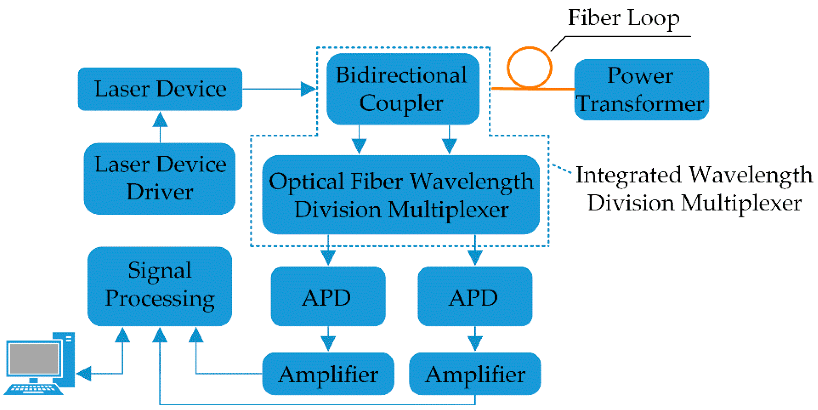
The working process of the optical fiber temperature sensor is shown in Figure 2. The pulsed laser enters the fiber through one end of the integrated wavelength division multiplexer (involving a 1 × 2 bidirectional coupler (BDC) and an optical fiber wavelength division multiplexer (OWDM)). Then its back scattering will be divided into Stokes and anti-Stokes Raman light by the integrated wavelength division multiplexer. After the photoelectric conversion in avalanche photodiode (APD) and high-speed analog-to-digital conversion, the processed signal will be delivered to a computer for temperature demodulation and data storage to achieve online distributed temperature measurement [30].

3. Development of the DOFS Integrated Power Transformer and Platform Setup

3.1. Design of the Distributed Optical Fiber Sensor Laying Scheme

The transformer prototype developed in this paper adopts a layered winding structure and its specific parameters are listed in

Table 1. Specifications of the transformer and the distributed optical fiber sensor (DOFS).

Power Transformer Prototype		DOFS
Rated capacity	200 kVA	Temperature resolution	<0.5 °C
Rated voltage	35 kV/400 V	Temperature accuracy	<1.0 °C
Rated current	3.3 A/288.7 A	Positioning accuracy	80 cm
Core type	Shell	Operating temperature range	−30–270 °C
Cooling method	ONAN	Response time	2–10 s
HV winding size	Height: 465 mm	Fiber type	multimode fiber
	Width: 310 mm	Fiber size	50/125/250/900 μm 1
LV winding size	Height: 460 mm	Fiber material (shealth/coating)	ETFE/PI
	Width: 186 mm	Effective monitoring range	2 km

¹ The size is fiber core/cladding/coating layer/sheath in external diameter.

. The detecting equipment is a commercial product (BY-DTS-4020, Weihai Beiyang Optoelectronic Info-Tech Co. Ltd., Weihai, China) and the relative parameters of the optical fiber and the instrument are also listed below. The high voltage (HV) winding utilizes the round copper wire while the low voltage (LV) winding uses the composite wire. The optical fiber laying scheme on the windings is shown in Figure 3.

The LV winding of the 35 kV transformer is composed of composite conductors, the unit of which consists of six parallelly flat copper wires. This leaves no oil ducts between each adjacent wire (as shown in Figure 3a). Temperature sensing can be realized by attaching the optical fiber to the wire surface of the outermost turn. Actual field experience shows that the optical fiber will be highly integrated with the winding due to the friction and stress generated from the laying process. In our experiment, the fiber did not break and the mechanical stress was moderate all the time. Meanwhile, a layer of insulating paper will be wrapped around the fiber composite wire to weaken the negative deviation of measurement caused by the cooling medium.

The HV winding is made up by enameled round copper conductors, which also means the direct contact between adjacent wires. For the convenience of fiber laying, a layer of insulating paper (0.2 mm) will be applied to the surface of the winding in advance, after which the optical fiber will be spirally winded on the paper closely attached to the wire (as exhibited in Figure 3b). The remaining steps are the same as aforesaid.

Through the high integration and close contact of the DOFS and the winding wire, the temperature of the designed optical fiber will be synchronized with the adjacent conductor during the actual operation of a transformer. Thus, the real time distributed temperature monitoring of the whole winding can be achieved. Meanwhile, a pulley guide should be utilized during the fiber laying process to ensure that the DOFS is evenly winded and closely adheres to the winding. The optical fiber was laid between the wire and the insulating paper, which will maintain the original winding structure and helps to buffer the possible vibrations and knocks during the manufacturing process. The iron core limbs and the inner wall of the oil tank were also uniformly winded by the distributed optical fiber sensors. The whole system is based on Raman scattering and it is only temperature-related, which means that the mechanical stress or the possible vibrations will not cause any interference.

3.2. Pre-Experiments

To ensure that the optical fiber works stably under the high temperature environment of transformer and has good compatibility with transformer oil, in our former series work [31], the safety test was performed through the accelerated thermal aging method (the optical fiber was immersed in the transformer oil at 130 °C for 576 h) which can be considered as equal to the fiber working continuously for 21 years under the normal operation of transformers according to IEC standards [13]. Tetrafluoroethylene (ETFE) and polyimide (PI) were finally selected as the optical fiber sheath and coating layer material due to their stable performance after the long-term aging process in the insulating oil. Meanwhile, the electric performance of the selected optical fiber was also qualified for the actual operating of a transformer due to its good insulation properties [11].

To furtherly test the hot region measuring accuracy of the as designed DOFS composite transformer windings, a temperature-rise experiment was performed on an assembled winding. The schematic diagram of the test platform is shown in Figure 4.

The distributed optical fiber sensor was fixed upon the outermost turn of winding with insulating paper, while the inner side of the winding wire was closely adhered to a heating tape to realize the temperature controlling. The heating tape adopted multi-point sampling through thermocouples to ensure that the temperature control error would reach 0.1 °C. The hot region detecting accuracy was explored by heating the discontinuous winding turns to different stable states (55 °C to 75 °C every 5 °C a state) and the measuring results are shown in Figure 5.

The experimental test shows that the as designed DOFS composite winding has a spatial resolution of 0.8 m (each hot region is 3.2 m wide and consists of four sampling points) and a temperature accuracy less than 0.3 °C. For the continuously winded windings inside the transformer, this accuracy is sufficient to locate the exact local overheating turn. Meanwhile, there is no oil passages between each adjacent wire in a layered structure winding, thus, the temperature along windings will be uniform and continuous. In the case of densely winded DOFS, massive data can be hereby obtained and interpolation method can be utilized to estimate the temperature where located under the spatial resolution.

The commercial product has already integrated a section of calibrating optical fiber inside and the reference temperature is stable according to the manufacturer. However, the equipment was also calibrated before the experiment. The temperature calibration was conducted through the thermostatic bath with a temperature error of 0.01 °C. Also, in the actual experiments, a section of fiber was exposed directly into the ambient environment and it was also compared with the thermocouples (exhibited in Figure 6). The ambient temperature detecting error (in average) was less than 0.3 °C, indicating that the instrument was reliable.

3.3. Platform Setup

The distributed optical fiber sensor integrated power transformer was fabricated based on the aforesaid laying schemes and it was in strict accordance with the normal manufacturing process. An optical fiber flange was sealed on the oil tank for signal extraction. The transformer prototype was up to standard for power grid operation through the corresponding ex-factory tests performed strictly according to the relevant IEC industry standards [13] (including induced over voltage withstand test, power-frequency voltage withstand test, tightness test, load loss and no-load loss measurement, dielectric routine tests, etc.).

It serves as a strong proof that the as designed distributed optical fiber sensor enjoys a high safety and stability inside the transformers and can be furtherly used in actual industrial application. The real time internal distributed temperature information was obtained through the temperature-rise test. The optical fiber was connected to an analysis equipment through the fiber flange. The sensing framework is shown in Figure 7 and the field application is exhibited in Figure 8.

4. Actual Detected Temperature and Numerical Simulation Results

4.1. Fully Distributed Internal Temperature Revelation

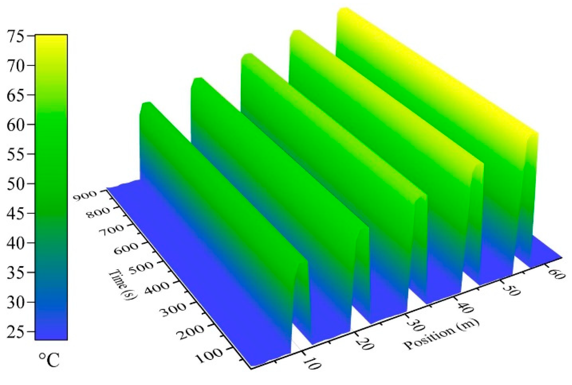
The temperature-rise test was strictly performed according to the corresponding IEC standard [13], simultaneously, the spatiotemporal temperature changes inside the operating transformer were also monitored in a distributed manner. The temperature-rise test was performed with the short-circuit method. It was composed of two steps, that is, applying total losses (first 8 h) and applying the rated current (the last hour). The as designed optical fiber sensor displays an effective sensing performance under the complex thermal conditions inside the power transformer and works stably all the time. The fiber laying length of each monitoring area is also exhibited in Figure 9.

For all the windings, the sensing fibers were connected with each other through the optical fiber patch cord on the outer side of the fiber flange (data of these extra fibers are not included in the results). The temperature distribution of the iron core limbs and the oil tank inside wall are shown in Figure 10.

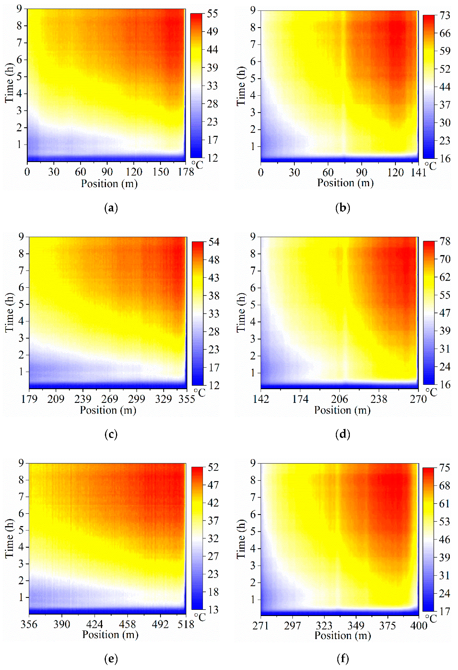
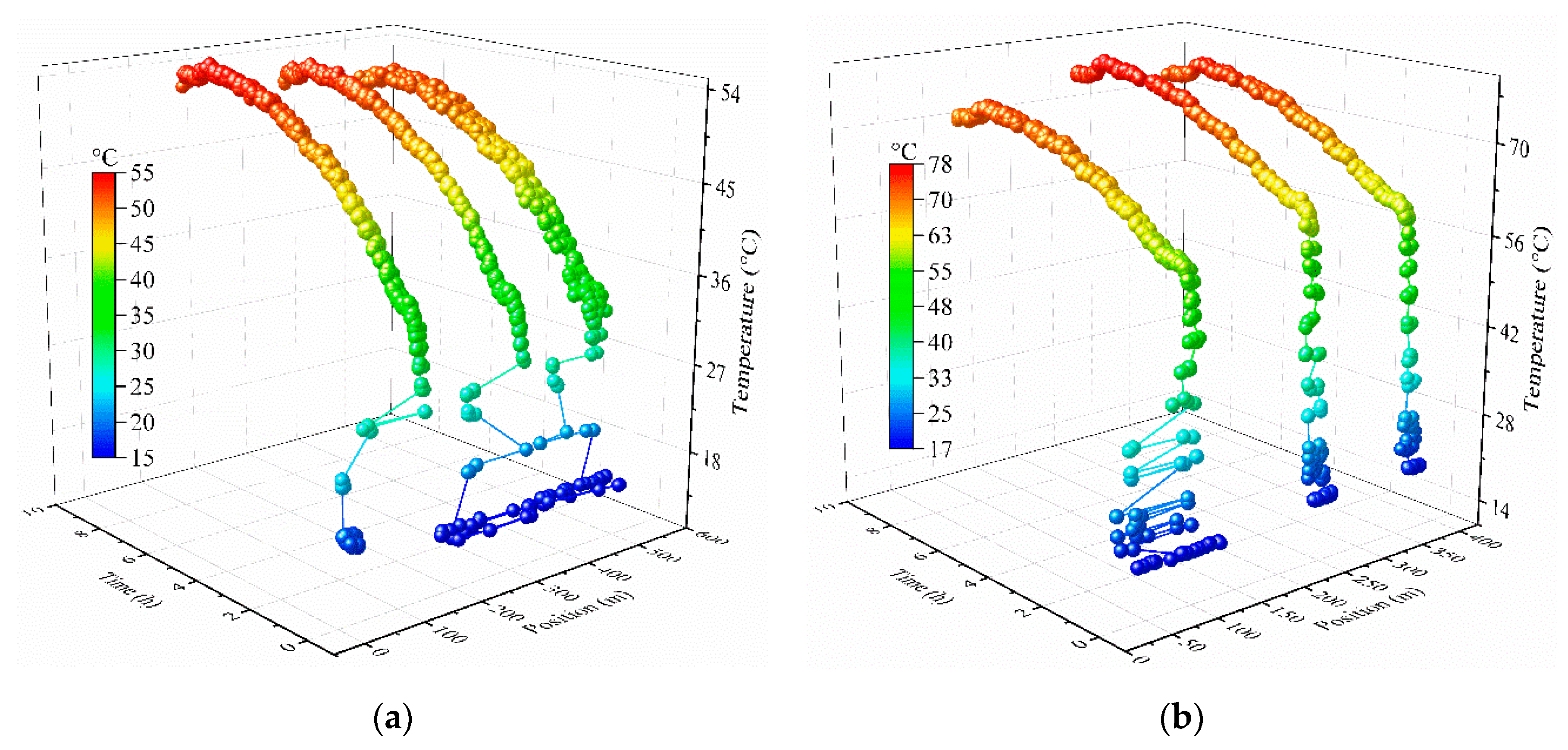
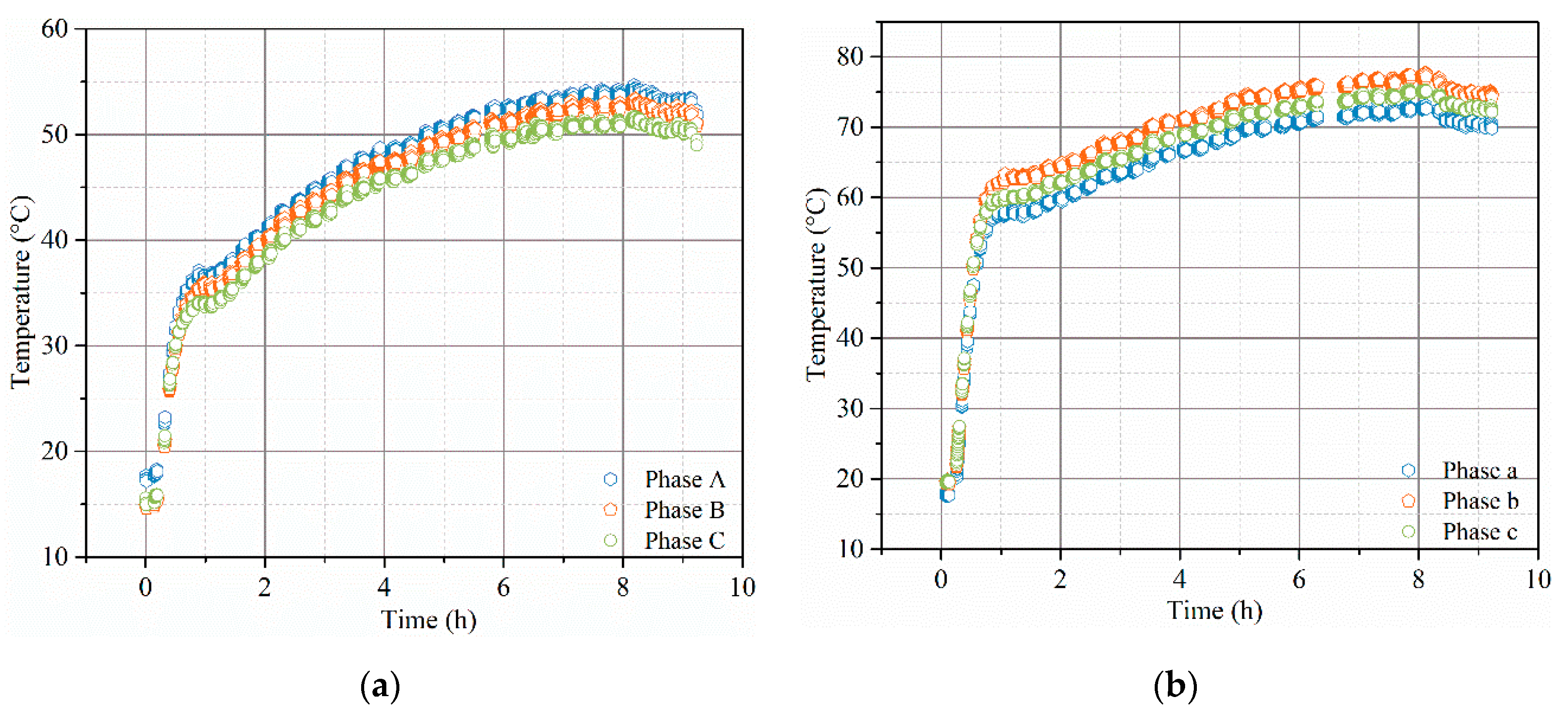
As for Figure 9a,c,e, the HV winding temperature presents an increasing trend with the height (the fiber was uniformly and spirally winded along the winding surface, so the fiber length can be normalized to the percentage of winding height). The hotspot gradually appeared after 3 h (80% of the highest temperature), around 44 °C, 43 °C, and 42 °C for phase A, B, and C, respectively. At the end of first step (8 h), the hotspot appeared at around 89%, 90%, and 91% of the winding height for phase A, B and C, respectively.

The LV winding displays a higher temperature compared to the HV winding due to its higher current, as shown in Figure 9b,d,f. The temperature increases with the winding height except for a downtrend in the top area, which may be caused by its relatively better heat dissipation conditions. The hotspot gradually arose after 2 h, almost 60 °C located at 85~92% of the winding height. The hotspot continued to spread to a larger region with the passage of time. And at 8 h, the hotspot for phase A, B, and C appeared at 88%, 91% and 88% of the winding height, respectively.

For the core limbs, exhibited in Figure 10a–c, the temperature distribution shows a positive correlation with the height for each phase. The hotspot appeared between 94% and 96% of the limb height for phase A, B, and C, respectively. However, there is little magnetic flux in the iron core during the short-circuit temperature-rise test and thus, the detected temperature may have a lower value compared to the actual situations. 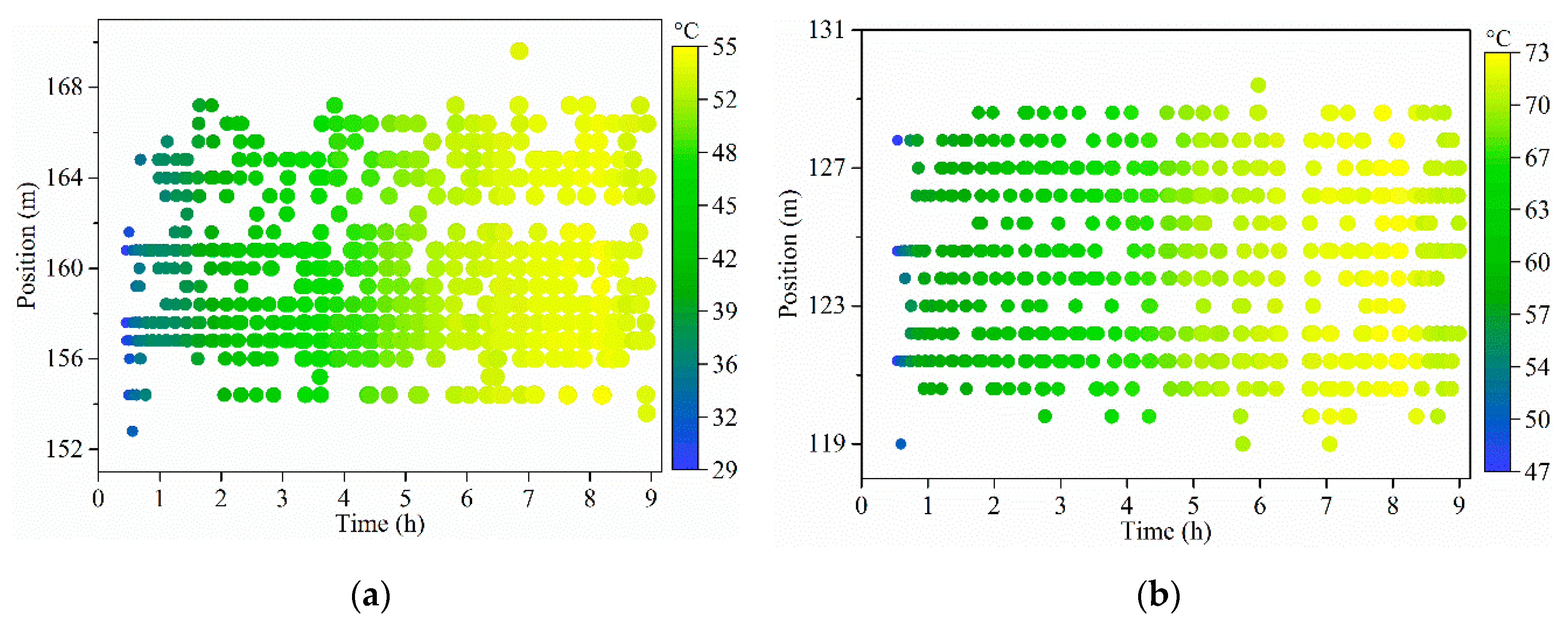The temperature along the inner wall of oil tank is shown in Figure 10d, which displays an increasing trend with time. However, the temperature distributed in an uneven way due to the continuously unstable oil flows along the tank wall and the hotspot appeared alternately on the upper or lower part of tank.

The hotspots of all the windings were closely monitored and continuously located, as exhibited in Figure 11. And the DOFS detecting results are compared with the IEC traditional calculating results in

Table 2. Hotspot detecting results compared with the IEC calculation.

Monitoring Method		Phase A		Phase B		Phase C
		Pos. 1 (%)	Temp. (°C)	Pos. 1 (%)	Temp. (°C)	Pos. 1 (%)	Temp. (°C)
DOFS	HV winding	89.5	54.8	90.2	53.7	91.1	51.9
	LV winding	88.4	72.9	91.3	77.8	88.7	74.8
	Core limb	94.3	52.9	94.4	53.7	96.2	50.9
	Oil tank	Tmax: 66.2 Pos.: upper or lower part
IEC method 2	HV winding	Pos.: cannot be obtained Temp.: 57 °C
	LV winding	Pos.: cannot be obtained Temp.: 79 °C
	Core limb	cannot be obtained
	Oil tank	cannot be obtained

¹ On average and within 2% fluctuation (possibly caused by the oil flows). ² Based on thermocouples and assumes that the hotspot always appears at the top of the windings and there is no difference between three phases [13].

.

As shown in Figure 11, the hotspots gradually came to a steady position after around 1 h for both the HV and LV windings. It can be possibly attributed to the fact that the oil gradually started to circulate at around 1 h. Before this time, the cold oil has a relatively large viscosity and there is almost no heat convection process inside the transformer, leading to a random position of the hotspot.

The actual status and life expectancy of a transformer is mainly determined by its insulation condition which is directly influenced by the hotspot temperature (HST). According to the traditional IEC calculation [13], the hotspot always appears at the top of windings with a relatively higher temperature, which may be attributed to the ignoration of the top area heat dissipation conditions in its idealized model. In fact, the cooling conditions in top area exhibit a great impact and cannot be easily ignored, as shown in Table 2, which will cause different shifts of hotspot location for different windings. Meanwhile, the IEC standard model also cannot obtain the distributed temperature data for different windings and lacks information about the iron core, oil tank, etc.

Obviously, the actual internal temperature distribution exhibits a strong position dependence, which can be possibly attributed to the different surrounding circumstances, such as irregular oil flows, various structural components, etc. Thus, the point-type detecting method would inevitably exist huge monitoring blind zones, leaving hidden dangers for the transformer’s safe operation.

Thus, the direct contact detection of DOFS is of great significance for the field applications compared to the traditional model-based calculation and point-to-point measuring methods.

The hotspot spatial distribution (phase A) and the transient temperature changes are also exhibited in Figure 12 and Figure 13.

The transient hotspot temperature showed a rapid increase before 1 h and then a slow upward trend. This phenomenon was caused by the insulating oil flow. At the very start, the cold oil was static, resulting in a fast local temperature rise (no flow means no heat convection). However, with the heat generated from windings continuing to accumulate, once the oil lifting force was larger than its gravity (1 h for this transformer), the static oil which carried lots of heat, began to circulate. This process explains the slow ascent of the temperature in the later part.

4.2. Finite Elelment Simulation Results

The revelation of the distributed temperature information inside an operating power transformer has provided massive detailed data for both researchers and field staff. However, the DOFS detecting method only has great advantages in the temperature sensing and it is still hard to fully understand what is happening inside the power transformer. Thus, the FEM (Finite Element Method) has been utilized to further analyze the internal physical process.

The transformer internal transient process was mainly focused in this simulation based on the hydrokinetics theories. The corresponding parameters used in the calculation are all from the manufacturers and are listed in

Table 3. Corresponding parameters for the simulation.

Properties	Density (kg·m−3)	Heat Capacity (J·kg−1·K−1)	Thermal Conductivity (W·m−1·K−1)
Tank/Fins	7900	460	47
Windings	8940	386	340
Cardboards	900	2000	0.21
Washers	750	2310	0.17
Blocks	960	1720	0.13

. The simulation results are exhibited in Figure 14.

According to the real structure of the studied 35 kV oil-immersed power transformer, a 3D thermal-fluid simulation model has been established. The calculation model maintains as much as structural components as possible, such as wood padding blocks, insulation cardboards, detailed iron core (composed of many layers of laminates), insulation washers, cooling fins, oil tank, windings, etc. However, it is impossible to totally and accurately reconstruct a real transformer due to the model complexity and the calculating time (or rather the convergence). Thereby, some necessary simplifications are inevitable. In this model, the windings are considered as coaxial cylinders, ignoring the detailed electromagnetic wire structures and the insulating papers wrapped around due to that it has adopted the layered winding structure. This simplification can leave out plenty of tiny components which only add the calculating difficulties and weaken the convergence.

The whole simulation was based on the COMSOL MUTIPHYSICS software (5.4, COMSOL AB, Stockholm, Sweden) and it took around 60 h according to our current hardware facility. The whole model has around 6 million elements in total, including 1.66 million mesh vertices, 70 thousand edge units, etc. The mesh independency was also proven when further increasing the element density (no more than 3% changes in the result). Meanwhile, the structured grid (mainly the hexahedral elements) and unstructured grid (basically the tetrahedral elements) were applied for different areas according to their characteristics.

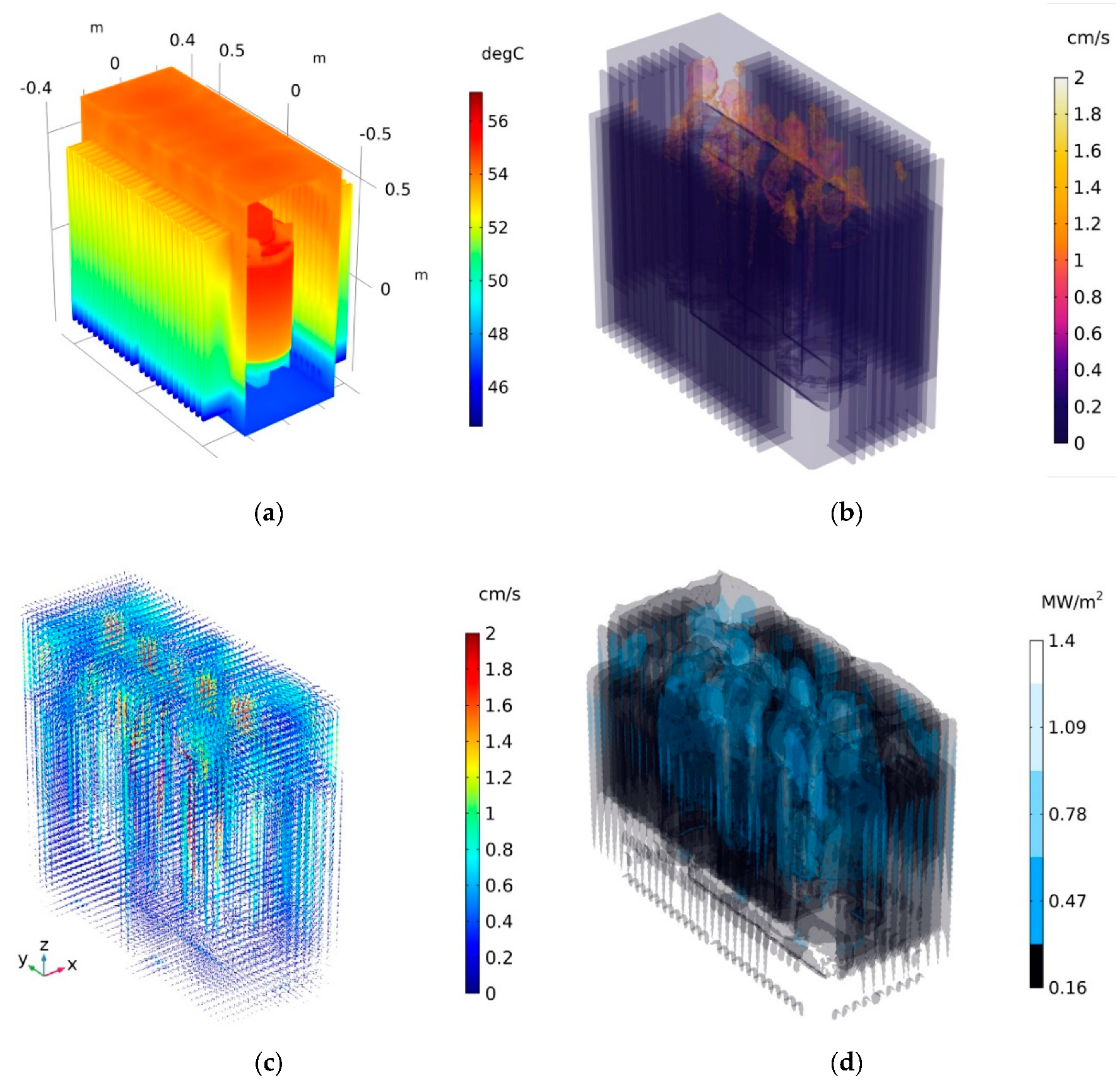
The thermal field transient simulation result (Figure 14a) showed a similar temperature distribution to the actual detected data. The HV winding hottest temperature reached about 57 °C, a little higher than the measured value. The flow field simulation result is exhibited in Figure 14b. There were several obvious vortexes appearing in the top area of the windings with a maximum flow velocity of 2 cm/s. For an ONAN power transformer, the circulation of insulating oil is mainly driven by the heat generated from the windings. Thus, the heated oil flows tend to climb up along the windings or the cardboards and gather in the top area where the heat emission conditions are relatively better. Then, part of the cooled oil begins to sink along the cooling fins while the rest would fall down directly and meet the upward streams to continuously form the vortexes (shown in detail in Figure 14c). The thermal flux distribution, displayed in Figure 14d, shows a similar process with the fluid field that the main heat flux is basically along the windings and reaches the highest value in the top area (the total heat exchange along the fins is also very active but it is not obvious when split into each one). The internal heat convection process is almost completed by the circulating oil and it is thus not strange that these two field simulations share a similar distribution.

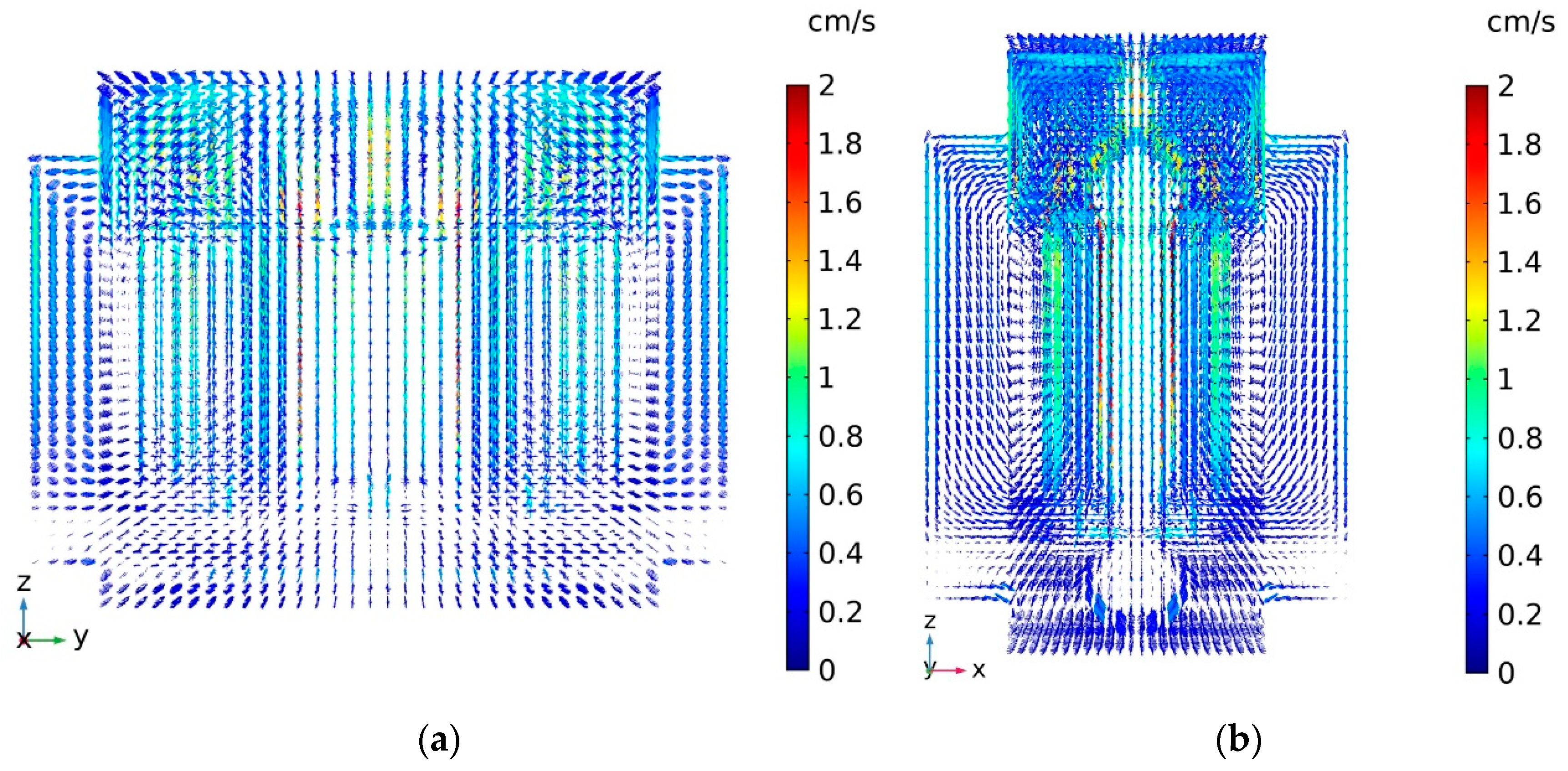
The vector diagram of the oil streams is displayed in Figure 15, where different perspectives are presented to aid further understanding.

The flow vectors exhibit a same whole-region oil circulation with the aforesaid process. Indeed, the relatively good cooling conditions in the winding top area would have a considerable impact on the hotspot locations, which is usually ignored by the field operation and maintenance staff or the manufacturers. Also, the real location of the winding hotspot tends to appear at around 90% of the winding height rather than the winding top according to our simulation and actual detected data.

5. Conclusions

In this paper, the DOFS was applied inside an operating power transformer and verified by the corresponding tests. Then, the transformer with a completely internal temperature sensing capability was successfully developed and qualified for actual application through the ex-factory type tests. The internal temperature was obtained in a distributed manner and it can serve as an important reference for both the field operation staff and the relevant engineers.

From this research, it was proven that the distributed optical fiber sensors can be applied into the power transformers for a spatiotemporally continuous temperature monitoring with a space resolution of 80 cm and temperature accuracy less than 0.5 °C. For the large transformers, the spatial positioning accuracy is enough to locate the exact overheated winding turn. For the small transformers, especially the ones with layered winding structure, the proposed densely winded optical fiber laying scheme is possibly a practical way to obtain the temperature where located under the spatial resolution.

Meanwhile, the real time internal temperature revelation shows that the hotspot real location is more likely at 90% of the winding height rather than the conventional cognition which asserts the hottest region is always at the winding top. The followed numerical simulation may partially account for this 10% deviation from the fluid field and thermal flux perspective.

In conclusion, the distributed sensing technology displays a promising future in the power transformer online temperature monitoring and may play an increasingly important role in the future electrical apparatus field.